Analytical Investigation of Viscoelastic Stagnation-Point Flows with Regard to Their Singularity

Abstract

Singularities in the stress field of the stagnation-point flow of a viscoelastic fluid have been studied for various viscoelastic constitutive models. Analyzing the analytical solutions of these models is the most effective way to study this problem. In this paper, exact analytical solutions of two-dimensional steady wall-free stagnation-point flows for the generic Oldroyd 8-constant model are obtained for the stress field using different material parameter relations. For all solutions, compatibility with the conservation of momentum is considered in our analysis. The resulting solutions usually contain arbitrary functions, whose choice has a crucial effect on the stress distribution. The corresponding singularities are discussed in detail according to the choices of the arbitrary functions. The results can be used to analyze the stress distribution and singularity behavior of a wide spectrum of viscoelastic models derived from the Oldroyd 8-constant model. Many previous results obtained for simple viscoelastic models are reproduced as special cases. Some previous conclusions are amended and new conclusions are drawn. In particular, we find that all models have singularities near the stagnation point and most of them can be avoided by appropriately choosing the model parameters and free functions. In addition, the analytical solution for the stress tensor of a near-wall stagnation-point flow for the Oldroyd-B model is also obtained. Its compatibility with the momentum conservation is discussed and the parameters are identified, which allow for a non-singular solution.

1. Introduction

The working fluids encountered in practical applications and industry are often non-Newtonian, and research on this type of fluids has been conducted for decades. In theoretical research, a variety of non-Newtonian fluid models has developed [1]. One group of these models is of the rate type which involves differential transport equations for the stress tensor. As these models are highly complex and mostly non-linear, exact analytical solutions can only be obtained for very special flow cases. Many theoretical works limit themselves to investigating the distribution of stress tensor in simple canonical viscoelastic flows by means of relatively simple models, such as the Oldroyd-B and Maxwell-B model, see, e.g., [2,3,4]. A classical model problem in this context, and also to be considered presently, is the similarity solution for the velocity field in a stagnation-point flow described, e.g., in [5]. Therein, the velocity distribution is usually assumed in the form $(u,v)=(x{f}^{\prime }\left(y\right),-f\left(y\right))$, though for a wall-free stagnation-point flow or a creeping stagnation-point flow far away from the wall, the velocity profile reduces to $f\left(y\right)=ay$, i.e., $(u,v)=(ax,-ay)$, where a is constant rate of the strain. Under this assumption, Phan-Thien [6,7] obtained exact solutions to the plane and axisymmetric stagnation-point flows for both Maxwellian and Oldroyd-B fluids, respectively, where the governing equations were reduced to a system of ordinary differential equations. It was shown that in a stagnation-point flow with a certain Weissenberg number, there is a singularity in the stress field. Renardy [8] analyzed a steady creeping flow of the upper convected Maxwell (UCM) fluid, in which the shear stress was assumed to be zero, and the normal stress depended only on the transverse coordinate of the outflow. His solution demonstrated that a singularity exists not only at the stagnation point, but also along the entire streamline passing the stagnation point downstream. Thomases et al. [9] used the same ansatz for the velocity field and solved the stress field of an Oldroyd-B fluid by using the method of characteristics. Their results showed that the behavior of the solutions is very sensitive to the Weissenberg number. However, the exact analytical solutions were only constructed for the model equations of the stress field without considering the compatibility with the momentum conservation equation. Cruz et al. [10] obtained a general analytical solution for a steady planar extensional wall-free stagnation-point flow of a viscoelastic fluid described by the UCM model. This solution depends on both space coordinates, and represents an extension of the previous solutions considering only the dependence of the transverse coordinate. Recently, Meleshko et al. [11] extended the analysis of the stress distribution in a wall-free stagnation-point flow from the UCM model to the Johnson–Segalman model and also took the momentum conservation equation into account. Their solution demonstrates that the Johnson–Segalman model has a non-removable logarithmic singularity.

In a near-wall stagnation-point flow, the velocity must satisfy the no-slip condition at the wall, so the velocity profile for the wall-free stagnation-point flow, i.e., $(u,v)=(x{f}^{\prime }\left(y\right),-f\left(y\right))$ with $f\left(y\right)=ay$, is here no longer suitable. In this case, the function $f\left(y\right)$ could take the form of $f\left(y\right)=a{y}^n$ with $n>1$ for an impermeable wall located at $y=0$. Under the simplest assumption $f\left(y\right)=a{y}^2$, Becherer et al. [12] and Van Gorder et al. [13], respectively, considered an UCM fluid and presented the exact solutions to the coupled PDEs of the viscoelastic stress. However, they did not analyze the compatibility of their solutions with the momentum conservation equation. Van Gorder [14] analyzed the same problem and showed that the solution for the stress components fails to satisfy the momentum conservation equation except in the linear case $f\left(y\right)=-ay$, corresponding to a wall-free stagnation-point flow. Therefore, to investigate near-wall stagnation-point flows, a more general velocity profile obeying the momentum conservation has to be proposed. All the models mentioned above can be derived from the Oldroyd 8-constant model, and many other models are also special cases of the Oldroyd 8-constant model [15]. It is interesting to investigate whether the other viscoelastic models have similar singularities as the Oldroyd-B, Maxwell-B and Johnson–Segalman models. For this purpose, we will search for exact analytical solutions for the Oldroyd 8-constant constitutive framework of a wall-free stagnation-point flow satisfying the compatibility with the conservation of momentum by means of the method of characteristics and analyze the effect of various model parameters on the solutions with regard to their singularity. Many conclusions previously obtained by other researchers for simple viscoelastic constitutive models are either confirmed or rectified. Some new conclusions are drawn. In particular, we find that all models have singularities near the stagnation point and most of them can effectively be avoided by appropriately choosing the model parameters and free functions. For the near-wall stagnation-point flow satisfying the no-slip conditions, it is impossible to analytically solve the constitutive equations of the Oldroyd 8-constant model. Instead, we focus on the Oldroyd-B model and analyze the compatibility of the solution with the momentum conservation equation.

2. Model Equations

2.1. Conservation Equations

The balance equation of momentum and mass conservation for an incompressible fluid take the form:

$$\rho \frac{D\mathbf{u}}{Dt}=\nabla ·\sigma +\rho \mathbf{f},$$

(1)

$$\nabla ·\mathbf{u}=0,$$

(2)

where $\rho$ is the fluid density, $\mathbf{u}$ the flow velocity, $\sigma$ is the Cauchy stress tensor, and $\mathbf{f}$ the volume force which is neglected in the present study. For a Maxwell fluid, $\sigma$ can be split in two parts:

$$\sigma =-p\mathbf{I}+{\mathbf{T}}_p,$$

(3)

where ${\mathbf{T}}_p$ is the polymetric stress contribution and p the dynamic pressure. For an Oldroyd-type fluid, a Newtonian stress part with a viscosity ${\eta }_s$ is added to the total stress and the Cauchy stress tensor is given by

$$\sigma =-p\mathbf{I}+2{\eta }_s\mathbf{D}+{\mathbf{T}}_p=-p\mathbf{I}+\mathbf{T}.$$

(4)

where $\mathbf{D}=\frac{1}{2}({\nabla \mathbf{u}}^T+\nabla \mathbf{u})$ is the symmetric rate-of-strain tensor. $\mathbf{T}$ is called the deviatoric stress tensor with $\mathbf{T}=2{\eta }_s\mathbf{D}+{\mathbf{T}}_p$.

2.2. The Oldroyd 8-Constant Model

The most general linear viscoelastic model is the Oldroyd 8-constant model [16] described by

$$\begin{array}{c}\hfill \mathbf{T}+{\lambda }_1\stackrel{\circ }{\mathbf{T}}+{\mu }_0\left(tr\mathbf{T}\right)\mathbf{D}-{\mu }_1\left(\mathbf{T}\mathbf{D}+\mathbf{D}\mathbf{T}\right)+{\nu }_1\left[tr\left(\mathbf{T}\mathbf{D}\right)\right]\mathbf{I}\\ \hfill =2{\eta }_0[\mathbf{D}+{\lambda }_2\stackrel{\circ }{\mathbf{D}}-2{\mu }_2{\mathbf{D}}^2+{\nu }_{2}tr\left({\mathbf{D}}^2\right)\mathbf{I}],\end{array}$$

(5)

where ${\lambda }_1,{\lambda }_2,{\mu }_0,{\mu }_1,{\mu }_2,{\nu }_1,{\nu }_2$ are material constants with the dimension of time. ${\eta }_0$ is the total viscosity split by ${\eta }_0={\eta }_p+{\eta }_s$ and ${\eta }_p$ is the polymer contribution to the viscosity. $\stackrel{\circ }{\mathbf{T}}$ is the corotational objective time derivative of $\mathbf{T}$ defined as

$$\stackrel{\circ }{\mathbf{T}}:=\frac{d\mathbf{T}}{dt}-\mathbf{W}\mathbf{T}+\mathbf{T}\mathbf{W},$$

(6)

where $\mathbf{W}=\frac{1}{2}({\nabla \mathbf{u}}^T-\nabla \mathbf{u})$ is the skew-symmetric vorticity tensor. Giesekus [1] has extended the Oldroyd 8-constant model by adding the term ${\nu }_0\left(tr\mathbf{T}\right)\mathbf{I}$ to the left-hand side of (5), but this extension will not be considered in the present investigation.

Most viscoelastic models can be derived from the Oldroyd 8-constant model [15]. For example, setting ${\mu }_1={\lambda }_1$, ${\mu }_2={\lambda }_2=\frac{{\eta }_s}{{\eta }_0}{\lambda }_1$, and ${\mu }_0={\nu }_1={\nu }_2=0$ in (5) gives the Oldroyd-B model:

$$\mathbf{T}+{\lambda }_1\stackrel{▽}{\mathbf{T}}=2{\eta }_0\left(\mathbf{D}+{\lambda }_2\stackrel{▽}{\mathbf{D}}\right)$$

(7)

where the symbol $\stackrel{▽}{}$ is the upper-convected time derivative, defined by

$$\stackrel{▽}{\mathbf{T}}:=\frac{d\mathbf{T}}{dt}-\nabla {\mathbf{u}}^T·\mathbf{T}-\mathbf{T}·\nabla \mathbf{u}.$$

(8)

Usually, a retardation parameter is defined by $\beta =\frac{{\eta }_p}{{\eta }_0}\in [0,1]$. $\beta =0$ corresponds to a Newtonian fluid, $\beta =1$ to a Maxwell fluid, and in between a Oldroyd fluid. If $\frac{{\eta }_s}{{\eta }_0}=1$, hence ${\lambda }_2={\lambda }_1$, the Oldroyd-B fluid reduces to the Newtonian fluid with the constitutive equation $\mathbf{T}=2{\eta }_s\mathbf{D}$. If ${\eta }_s=0$, hence ${\lambda }_2=0$, ${\eta }_0={\eta }_p$, $\mathbf{T}={\mathbf{T}}_p$, and the Maxwell-B model is obtained:

$${\mathbf{T}}_p+{\lambda }_1{\stackrel{▽}{\mathbf{T}}}_p=2{\eta }_p\mathbf{D}.$$

(9)

Combining the constitutive Equation (7) and the relation $\mathbf{T}=2{\eta }_s\mathbf{D}+{\mathbf{T}}_p$ for an Oldroyd fluid results in a constitutive relation in terms of ${\mathbf{T}}_p$, which is completely consistent with the expression of (9). However, in contrast to the Maxwell fluid, the Newtonian viscosity ${\eta }_s$ in the momentum equation of an Oldroyd-type fluid is not zero. More examples of viscoelastic models derived from the Oldroyd 8-constant model can be found in the Table II of [15].

We employed the dimensionless variables, which are scaled by the characteristic length $L_0$, strain rate a and viscosity ${\eta }_0$ as following:

$$\begin{array}{cc}\hfill & \tilde{\mathbf{x}}=\frac{\mathbf{x}}{L_0},\tilde{\mathbf{u}}=\frac{\mathbf{u}}{a{L}_0},\tilde{p}=\frac{p}{a{\eta }_0},\tilde{\mathbf{T}}=\frac{\mathbf{T}}{a{\eta }_0},Re=\frac{\rho a{L}_0^2}{{\eta }_0},W_1=a{\lambda }_1,\hfill \\ \hfill & W_2=a{\mu }_0,W_3=a{\mu }_1,W_4=a{\nu }_1,W_5=a{\lambda }_2,W_6=a{\mu }_2,W_7=a{\nu }_2,\hfill \end{array}$$

(10)

where $W_1,...,W_7$ are Weissenberg numbers and $Re$ the Reynolds number. Omitting the tilde symbol, the constitutive Equation (5) can be rewritten in the following dimensionless form:

$$\begin{array}{c}\hfill \mathbf{T}+W_1\stackrel{\circ }{\mathbf{T}}+W_2\left(tr\mathbf{T}\right)\mathbf{D}-W_3\left(\mathbf{T}\mathbf{D}+\mathbf{D}\mathbf{T}\right)+W_4\left[tr\left(\mathbf{T}\mathbf{D}\right)\right]\mathbf{I}\\ \hfill =2[\mathbf{D}+W_5\stackrel{\circ }{\mathbf{D}}-2W_6{\mathbf{D}}^2+W_{7}tr\left({\mathbf{D}}^2\right)\mathbf{I}].\end{array}$$

(11)

Then, the dimensionless Oldroyd 8-constant model (11) will be utilized for investigating the two-dimensional steady stagnation-point flows with regard to their singularities under different material parameter relations.

3. Analytical Solutions of a Wall-Free Stagnation-Point Flow and Their Singularities

For the velocity field of a two-dimensional steady stagnation-point flow, there exists a similarity solution described as

$$\mathbf{u}=(x{f}^{\prime }\left(y\right),-f\left(y\right)),$$

(12)

where $f\left(y\right)$ is an arbitrary function depending only on y [5,6]. In the case of a wall-free stagnation-point flow, the flow is a potential flow, which means $\nabla \times \mathbf{u}=0$. This leads to $f^{\prime \prime }\left(y\right)=0$, and further $f\left(y\right)=ay$. The parameter a stands for the constant rate of the strain and is employed in the non-dimensionalization, as shown in (10). Hence, the dimensionless velocity field is given by

$$\mathbf{u}=\left(x,-y\right).$$

(13)

The velocity field is symmetrical for both the x and the y axis, as shown in Figure 1, so we only need to consider the case with $x,y>0$ in the following analysis.

Figure 1. Sketch of the velocity field in a wall-free stagnation-point flow.

The stress tensor is symmetric and takes a two-dimensional form of:

$$\mathbf{T}=\left(\begin{array}{cc}{T}_{11}& T_{12}\\ T_{12}& T_{22}\end{array}\right).$$

(14)

Substituting (13) and (14) into (11), we obtain the following three scalar constitutive equations:

$$\begin{array}{ccc}& & W_{1}x\frac{\partial T_{11}}{\partial x}-W_{1}y\frac{\partial T_{11}}{\partial y}=(k_1-1)T_{11}-k_2{T}_{22}-k_3+2,\hfill \end{array}$$

(15)

$$\begin{array}{ccc}& & W_{1}x\frac{\partial T_{22}}{\partial x}-W_{1}y\frac{\partial T_{22}}{\partial y}=k_2{T}_{11}-(k_1+1)T_{22}-k_3-2,\hfill \end{array}$$

(16)

$$\begin{array}{ccc}& & W_{1}x\frac{\partial T_{12}}{\partial x}-W_{1}y\frac{\partial T_{12}}{\partial y}=-T_{12},\hfill \end{array}$$

(17)

where $k_1=2W_3-W_2-W_4$, $k_2=W_2-W_4$ and $k_3=4(W_6-W_7)$. It is to notice that $\stackrel{\circ }{\mathbf{D}}=0$ under the assumption of the velocity (13), so the Weissenberg number $W_5$ has not any influence on the stress field.

In the PDE system (15)–(17), Equation (17) for $T_{12}$ is uncoupled with (15), (16), and thus can be solved independently. The coupling of (15) and (16) for $T_{11}$ and $T_{22}$ depends on the value of $k_2$. If $k_2=0$, both the equations are decoupled and can be solved separately for $T_{11}$ and $T_{22}$. If $k_2\ne 0$, Equations (15) and (16) constitute a coupled PDE system with non-constant coefficients. In addition, the solutions of the PDE system (15)–(17) must also satisfy the compatibility condition derived by substituting (4), (13) and (14) into the rotation of the momentum Equation (1):

$$\frac{{\partial }^2{T}_{11}}{\partial x\partial y}-\frac{{\partial }^2{T}_{22}}{\partial x\partial y}-\frac{{\partial }^2{T}_{12}}{\partial x^2}+\frac{{\partial }^2{T}_{12}}{\partial y^2}=0.$$

(18)

In the following, the analytic solutions of the constitutive Equations (15)–(17) with consideration of the compatibility condition (18) will be derived, respectively, for the two cases $k_2=0$ and $k_2\ne 0$.

3.1. Case $k_2=0$

Many of the viscoelastic models derived from the Oldroyd 8-constant model (11) are characterized by $W_2=W_4$, i.e., $k_2=0$. Examples are the Oldroyd-B, Maxwell-B, Johnson–Segalman models. Their solutions are all contained in this part.

In the case of $k_2=0$, the three components of the stress tensor can be separately solved by using the method of characteristics. The characteristic equations of (15)–(17) are given by

$$\begin{array}{ccc}& & \frac{dx}{W_{1}x}=\frac{dy}{-W_{1}y}=\frac{d{T}_{11}}{(k_1-1)T_{11}-k_3+2},\hfill \end{array}$$

(19)

$$\begin{array}{ccc}& & \frac{dx}{W_{1}x}=\frac{dy}{-W_{1}y}=\frac{d{T}_{22}}{-(k_1+1)T_{22}-k_3-2},\hfill \end{array}$$

(20)

$$\begin{array}{ccc}& & \frac{dx}{W_{1}x}=\frac{dy}{-W_{1}y}=\frac{d{T}_{12}}{-1}.\hfill \end{array}$$

(21)

The values of $k_1-1$ and $k_1+1$, arising in (19) and (20) as the coefficients of $T_{11}$ and $T_{22}$, have a crucial effect on the structure of their solutions. Therefore, the solutions will be further investigated for the following three cases, respectively.

3.1.1. Case $(k_1-1)(k_1+1)\ne 0$

In this case, $k_1\ne \pm 1$, we can obtain the following solutions by solving the Equations (19)–(21):

$$\begin{array}{ccc}& & T_{11}=F_1\left(\psi \right)·y^{\frac{1-k_1}{W_1}}+\frac{k_3-2}{k_1-1},\hfill \end{array}$$

(22)

$$\begin{array}{ccc}& & T_{22}=F_2\left(\psi \right)·y^{\frac{1+k_1}{W_1}}-\frac{k_3+2}{k_1+1},\hfill \end{array}$$

(23)

$$\begin{array}{ccc}& & T_{12}=F_3\left(\psi \right)·y^{\frac{1}{W_1}}.\hfill \end{array}$$

(24)

$F_1\left(\psi \right)$, $F_2\left(\psi \right)$ and $F_3\left(\psi \right)$ are arbitrary functions of $\psi =xy$, and $\psi =const.$ represents the characteristic lines of the solutions. This result is consistent with that obtained by Van Gorder [14] for the stagnation-point flow of an upper convected Maxwell fluid, in which $k_1=2W_1$ and $k_3=0$.

Further satisfying the compatibility condition (18) yields the following restriction on functions $F_1$, $F_2$, and $F_3$:

$$\begin{array}{cc}\hfill & \left[\psi F_1^{\prime \prime }+\left(\frac{1-k_1}{W_1}+1\right)F_1^{\prime }\right]y^{-\frac{k_1}{W_1}}-\left[\psi F_2^{\prime \prime }+\left(\frac{1+k_1}{W_1}+1\right)F_2^{\prime }\right]y^{\frac{k_1}{W_1}}\hfill \\ \hfill & +\left[{\psi }^2{F}_3^{\prime \prime }+\frac{2}{W_1}\psi F_3^{\prime }+\frac{1}{W_1}\left(\frac{1}{W_1}-1\right)F_3\right]y^{-2}-F_3^{\prime \prime }{y}^2=0.\hfill \end{array}$$

(25)

The only way to satisfy this condition for any value of y is that all coefficients of $y^k$ vanish. This induces three different cases depending on the value of $\frac{k_1}{W_1}$. The case of $\frac{k_1}{W_1}=\pm 2$ corresponds to the Oldroyd and Maxwell fluids. Their solutions for Weissenberg number $W_1\ne \frac{1}{2}$ are covered in this investigation.

(i)

If $\frac{k_1}{W_1}=2$, only two restriction conditions for $F_1$, $F_2$, and $F_3$ can be obtained from (25), meaning that:

$$\begin{array}{ccc}& & \psi F_1^{\prime \prime }+\left(\frac{1}{W_1}-1\right)F_1^{\prime }+{\psi }^2{F}_3^{\prime \prime }+\frac{2}{W_1}\psi F_3^{\prime }+\frac{1}{W_1}\left(\frac{1}{W_1}-1\right)F_3=0,\hfill \end{array}$$

(26)

$$\begin{array}{ccc}& & \psi F_2^{\prime \prime }+\left(\frac{1}{W_1}+3\right)F_2^{\prime }+F_3^{\prime \prime }=0.\hfill \end{array}$$

(27)

Hence, $F_1$ and $F_2$ can be related to $F_3$ by

$$\begin{array}{ccc}& & F_1=-\psi F_3+\left(1-\frac{1}{W_1}\right)\int F_{3}d\psi +C_1{\psi }^{2-\frac{1}{W_1}}+C_2,\hfill \end{array}$$

(28)

$$\begin{array}{ccc}& & F_2=-{\psi }^{-1}{F}_3+\left(\frac{1}{W_1}+1\right){\psi }^{-\frac{1}{W_1}-2}\int {\psi }^{\frac{1}{W_1}}{F}_{3}d\psi +C_3{\psi }^{-\frac{1}{W_1}-2}+C_4,\hfill \end{array}$$

(29)

where $C_1$, $C_2$, $C_3$ and $C_4$ are arbitrary constants, and $F_3$ is still an arbitrary function of $\psi =xy$. To avoid the integral terms emerging in the above relations, we replace $F_3$ by another arbitrary function $F\left(\psi \right)$ as follows:

$$F_3={\left({\psi }^{1-\frac{1}{W_1}}{F}^{\prime }\right)}^{\prime }={\psi }^{-\frac{1}{W_1}}{\left(\psi F^{\prime }-\frac{1}{W_1}F\right)}^{\prime }.$$

(30)

Substituting (30) into (28), (29) and then into (22)–(24), results in the final solutions of the stress tensor:

$$\begin{array}{ccc}& T_{11}=& -x^{2-\frac{1}{W_1}}{F}^{\prime \prime }+C_1{x}^{2-\frac{1}{W_1}}+C_2{y}^{\frac{1}{W_1}-2}+\frac{k_3-2}{k_1-1},\hfill \end{array}$$

(31)

$$\begin{array}{ccc}& T_{22}=& -x^{-\frac{1}{W_1}}{y}^2{F}^{\prime \prime }+\frac{2}{W_1}{x}^{-\frac{1}{W_1}-1}y{F}^{\prime }-\frac{1}{W_1}\left(\frac{1}{W_1}+1\right)x^{-\frac{1}{W_1}-2}F\hfill \\ & & +C_3{x}^{-\frac{1}{W_1}-2}+C_4{y}^{\frac{1}{W_1}+2}-\frac{k_3+2}{k_1+1},\hfill \end{array}$$

(32)

$$\begin{array}{ccc}& T_{12}=& x^{1-\frac{1}{W_1}}y{F}^{\prime \prime }+\left(1-\frac{1}{W_1}\right)x^{-\frac{1}{W_1}}{F}^{\prime }.\hfill \end{array}$$

(33)

In a recent investigation by [17], the solution of a wall-free stagnation-point flow for the Maxwell fluid with $W_1\ne \frac{1}{2}$ satisfying the momentum equation was discovered. This corresponds to our solutions (31)–(33) with $k_1=2W_1$ and $k_3=0$. Physically, the components of the stress tensor should be limited everywhere, including at the stagnation point $(x,y)=(0,0)$ and at infinity. Hence, further restrictions on the arbitrary constants $C_1$, $C_2$, $C_3$, $C_4$ and the arbitrary function $F\left(xy\right)$ in the solutions are needed. To avoid the singularity of the stress tensor, Ref. [17] suggested the choice:

$$F\left(xy\right)={\left(xy\right)}^{2+\frac{1}{W_1}+\delta }{e}^{-b{\left(xy\right)}^2},C_1=C_2=C_3=C_4=0,$$

(34)

where $\delta >0$ and $b>0$. However, this choice (34) cannot prevent the singularity as was claimed. To demonstrate this, as an example, we substitute (34) into (33) resulting in:

$$T_{12}=\left[a_1+a_2{\left(xy\right)}^2+a_3{\left(xy\right)}^4\right]e^{-b{\left(xy\right)}^2}·{\left(xy\right)}^{1+\delta }·y^{\frac{1}{W_1}}=G\left(xy\right)·y^{\frac{1}{W_1}},$$

(35)

where $a_1=(2+\delta )(2+\delta +\frac{1}{W_1})$, $a_2=-2b(6+2\delta +\frac{1}{W_1})$ and $a_3=4b^2$ are constant coefficients. For $W_1>0$, the particular solution (33) has the following properties:

•

Along the characteristic curves $xy=0$ and $xy\to \infty$, $T_{12}\to 0$, no singularity occurs.

•

Along the characteristic curve $xy=c_0$, where $c_0$ is a non-zero finite constant, the value of $G\left(xy\right)$ is a bounded constant $G\left(c_0\right)$, while $y^{\frac{1}{W_1}}$ is singular at $y\to \infty$. An infinite shear stress $T_{12}$ arises in the region far away from the stagnation point ($y\to \infty$) and near the y-axis ($x\to 0$).

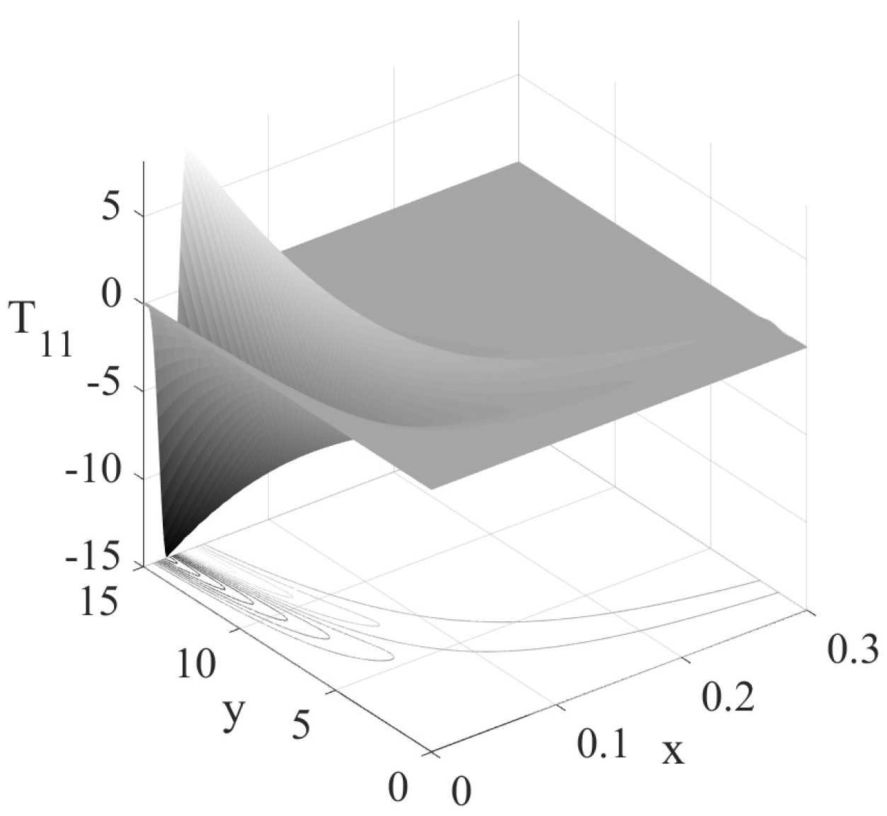
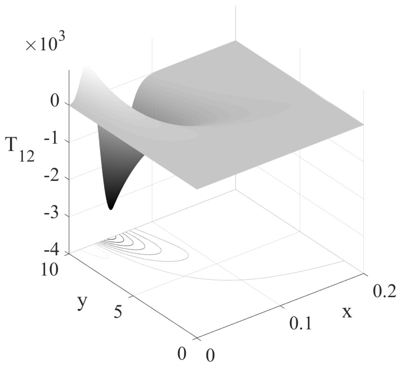
With the choice (34), similar singularities also appear in the stress tensor components $T_{11}$ and $T_{22}$ far away from the stagnation point, for $y\to \infty$ (but $x\to 0$) or $x\to \infty$ (but $y\to 0$). As an example, the corresponding stress components $T_{11}$ and $T_{12}$ excluding the constant part $\frac{k_3-2}{k_1-1}$ are presented in Figure 2 and Figure 3 for the case $W_1=0.25$, $\delta =2$ and $b=12$ with a much finer spatial resolution than [17] used. The present figures show that a singularity in the stress field may arise in the region far away from the stagnation point ($y\to \infty$) and near the y axis ($x\to 0$), as previously analytically recognized, while in [17], this tendency was invisible due to the rather coarse resolution employed.

Figure 2. Stress component $T_{11}$ with a spatial resolution of $x\in [0:0.001:0.3]$, $y\in [0:0.001:15]$.

Figure 3. Stress component $T_{12}$ with a spatial resolution of $x\in [0:0.001:0.2]$, $y\in [0:0.001:10]$.

Actually, the appearance of the singularity at $(x,y)\to (0,\infty )$ or $(x,y)\to (\infty ,0)$ is independent from the choice of the arbitrary function $F\left(xy\right)$. This can be easily recognized by observing the distribution of the stresses (31)–(33) along an arbitrary characteristic curve $xy=c_0$, where $c_0$ is non-zero finite constant. As an example, the term $x^{-\frac{1}{W_1}}{F}^{\prime }\left(xy\right)$ tends to be infinite at $(x,y)\to (0,\infty )$ for $W_1>0$ or at $(x,y)\to (\infty ,0)$ for $W_1<0$. These singularities are independent from the choice of $F\left(xy\right)$ and thus non-removable. However, possible singularity near the stagnation point $(x,y)\to (0,0)$ can be effectively prevented by choosing a reasonable function $F\left(xy\right)$, e.g., (34). This ensures that no singularity occurs in the stress field near the stagnation point. For a stagnation-point flow with the velocity field given by (13), the velocity becomes unbounded at $x\to \infty$ or $y\to \infty$ and is thus physically no longer meaningful. The singularity arising in the far field at $x\to \infty$ or $y\to \infty$ may not be relevant when a bounded stagnation-point flow is investigated. We should then focus on the analysis of singularity in a bounded area near the stagnation point.

(ii)

If $\frac{k_1}{W_1}=-2$, performing the similar steps as for the above case gives the solutions:

$$\begin{array}{ccc}& T_{11}=& x^{-\frac{1}{W_1}}{y}^2{F}^{\prime \prime }-\frac{2}{W_1}{x}^{-\frac{1}{W_1}-1}y{F}^{\prime }+\frac{1}{W_1}\left(\frac{1}{W_1}+1\right)x^{-\frac{1}{W_1}-2}F\hfill \\ & & +C_1{x}^{-\frac{1}{W_1}-2}+C_2{y}^{\frac{1}{W_1}+2}+\frac{k_3-2}{k_1-1},\hfill \end{array}$$

(36)

$$\begin{array}{ccc}& T_{22}=& x^{2-\frac{1}{W_1}}{F}^{\prime \prime }+C_3{x}^{2-\frac{1}{W_1}}+C_4{y}^{\frac{1}{W_1}-2}-\frac{k_3+2}{k_1+1},\hfill \end{array}$$

(37)

$$\begin{array}{ccc}& T_{12}=& x^{1-\frac{1}{W_1}}y{F}^{\prime \prime }+\left(1-\frac{1}{W_1}\right)x^{-\frac{1}{W_1}}{F}^{\prime }.\hfill \end{array}$$

(38)

Similarly, by reasonably choosing of $C_i$ ($i=1,2,3,4$) and $F\left(xy\right)$, singularity near the stagnation point can be avoided.

(iii)

If $\frac{k_1}{W_1}\ne \pm 2$, we obtain four equations for $F_1$, $F_2$ and $F_3$ from (25). Solving them and then substituting them into (22)–(24) yield:

$$\begin{array}{ccc}& & T_{11}=C_1{x}^{-\frac{1-k_1}{W_1}}+C_2{y}^{\frac{1-k_1}{W_1}}-\frac{k_3-2}{1-k_1},\hfill \end{array}$$

(39)

$$\begin{array}{ccc}& & T_{22}=C_3{x}^{-\frac{1+k_1}{W_1}}+C_4{y}^{\frac{1+k_1}{W_1}}-\frac{k_3+2}{1+k_1},\hfill \end{array}$$

(40)

$$\begin{array}{ccc}& & T_{12}=0.\hfill \end{array}$$

(41)

To prevent the singularity near the stagnation point $(x,y)=(0,0)$, only one of $C_1$, $C_2$ and one of $C_3$, $C_4$ need to be zero according to the relative relationship between $k_1$ and $W_1$. This results in a stress distribution that depends on only one coordinate x or y.

3.1.2. Case $k_1-1=0$

In this case, the coefficient of $T_{11}$ in (19) vanishes. The corresponding solution of $T_{11}$ is simply given by

$$T_{11}=\frac{k_3-2}{W_1}lny+F_1,$$

(42)

where $F_1$ is an arbitrary function of $\psi =xy$. The solutions of $T_{22}$ and $T_{12}$ remain the same as given in (22)–(24). Again, considering the compatibility condition, the final solutions are obtained depending on the value of $W_1$. All intermediate steps, which are similar to those in the last Section 3.1.1, are omitted.

(i)

If $W_1=\frac{1}{2}$, we obtain the solutions:

$$\begin{array}{ccc}& & T_{11}=2(k_3-2)lny-F^{\prime \prime }+C_{1}ln\left(xy\right)+C_2,\hfill \end{array}$$

(43)

$$\begin{array}{ccc}& & T_{22}=-x^{-2}{y}^2{F}^{\prime \prime }+4x^{-3}y{F}^{\prime }-6x^{-4}F+C_3{x}^{-4}+C_4{y}^4-\frac{k_3}{2}-1,\hfill \end{array}$$

(44)

$$\begin{array}{ccc}& & T_{12}=x^{-1}y{F}^{\prime \prime }-x^{-2}{F}^{\prime };\hfill \end{array}$$

(45)

The logarithmic singularity in $T_{11}$ caused by $lny$ at $y\to 0$ can only be avoided when $k_3=2$, i.e., $W_6-W_7=\frac{1}{2}$. In this case, the choice (34) for the arbitrary constants $C_i$ ($i=1,2,3,4$) and arbitrary function $F\left(xy\right)$ is still suitable to prevent the singularity near the stagnation point.

However, for the Oldroyd model, i.e., the case of $W_6-W_7=4(1-\beta )W_1$ with $0<\beta <1$ and for the Maxwell model, i.e., the case of $W_6-W_7=0$, the logarithmic singularity at the Weissenberg number $W_1=\frac{1}{2}$ is unavoidable. The similar conclusion was also drawn by [11] for Maxwell fluid.

(ii)

If $W_1\ne \frac{1}{2}$:

$$\begin{array}{ccc}& & T_{11}=\frac{k_3-2}{W_1}lny+C_{1}ln\left(xy\right)+C_2,\hfill \end{array}$$

(46)

$$\begin{array}{ccc}& & T_{22}=C_3{x}^{-\frac{2}{W_1}}+C_4{y}^{\frac{2}{W_1}}-\frac{k_3}{2}-1,\hfill \end{array}$$

(47)

$$\begin{array}{ccc}& & T_{12}=0.\hfill \end{array}$$

(48)

The singularity caused by the term $lny$ can only be avoided if $k_3=2$. In addition, $C_3$ also has to be zero to prevent the singularity at $xy\to 0$. This choice will cause a uniform stress field, which may be physically disputable.

3.1.3. Case $k_1+1=0$

Analogous to the last two subsections, the solutions in this case are distinguished for the following cases.

(i)

If $W_1=\frac{1}{2}$:

$$\begin{array}{cc}\hfill & T_{11}=x^{-2}{y}^2{F}^{\prime \prime }-4x^{-3}y{F}^{\prime }+6x^{-4}F+6C_1{x}^{-4}+C_2{y}^4-\frac{k_3}{2}+1,\hfill \\ \hfill & T_{22}=2(k_3+2)lny+F^{\prime \prime }+C_{3}ln\left(xy\right)+C_4,\hfill \\ \hfill & T_{12}=x^{-1}y{F}^{\prime \prime }-x^{-2}{F}^{\prime }.\hfill \end{array}$$

(49)

where the logarithmic singularity caused by $lny$ in $T_{22}$ could only be avoided with the extra restriction $k_3+2=0$. However, for the Oldroyd model there is $k_3=2(1-\beta )$ at $W_1=\frac{1}{2}$ with $<0\beta <1$ and for the Maxwell model $k_3=0$, so that logarithmic singularity is non-removable. The similar conclusion was also drawn by [11] for a Maxwell fluid.

(ii)

For $W_1\ne \frac{1}{2}$:

$$\begin{array}{cc}\hfill & T_{11}=C_1{x}^{-\frac{2}{W_1}}+C_2{y}^{\frac{2}{W_1}}-\frac{k_3}{2}+1,\hfill \\ \hfill & T_{22}=\frac{k_3+2}{W_1}lny+C_{3}ln\left(xy\right)+C_4,\hfill \\ \hfill & T_{12}=0.\hfill \end{array}$$

(50)

Similar to the last cases, the singularity in $T_{11}$ and $T_{22}$ can only be avoided at $k_3=-2$ with $C_i=0$ ($i=1,2,3$). This again corresponds to a uniform stress field and thus may be physically disputable.

3.2. Case $k_2\ne 0$

For some of the viscoelastic models derived from the Oldroyd 8-constant model $k_2$ is not zero, such as the Williams 3-constant Oldroyd model, Oldroyd-4-constant model, etc., details see [15]. For this case, the solution of $T_{12}$ remains the same as in (24). $T_{11}$ and $T_{22}$ need to be solved from the coupled PDE system consisting of (15) and (16) with non-constant coefficients.

Applying the method of characteristics, the PDE system reduces to the following ODE system:

$$\begin{array}{ccc}& & W_{1}y\frac{d{T}_{11}}{dy}=(1-k_1)T_{11}+k_2{T}_{22}+k_3-2,\hfill \end{array}$$

(51)

$$\begin{array}{ccc}& & W_{1}y\frac{d{T}_{22}}{dy}=-k_2{T}_{11}+(1+k_1)T_{22}+k_3+2,\hfill \end{array}$$

(52)

along the characteristic curves $xy=const.$ Furthermore, using the transformation:

$$y=e^{W_1\tilde{y}}$$

(53)

Equations (51) and (52) can be transformed into an ODE system with constant coefficients:

$$\begin{array}{ccc}& & \frac{d{T}_{11}}{d\tilde{y}}=(1-k_1)T_{11}+k_2{T}_{22}+k_3-2,\hfill \end{array}$$

(54)

$$\begin{array}{ccc}& & \frac{d{T}_{22}}{d\tilde{y}}=-k_2{T}_{11}+(1+k_1)T_{22}+k_3+2,\hfill \end{array}$$

(55)

or in matrix form:

$$\frac{d\mathbf{t}}{d\tilde{y}}=\mathbf{A}\mathbf{t}+\mathbf{b}$$

(56)

with:

$$\mathbf{t}=\left(\begin{array}{c}{T}_{11}\\ T_{22}\end{array}\right),\mathbf{A}=\left(\begin{array}{cc}1-k_1& k_2\\ -k_2& 1+k_1\end{array}\right),\mathbf{b}=\left(\begin{array}{c}{k}_3-2\\ k_3+2\end{array}\right).$$

(57)

Eliminating $T_{22}$ by combining (54) and (55), gives an second-order ODE with constant coefficients for $T_{11}$:

$$\frac{d^2{T}_{11}}{d{\tilde{y}}^2}-2\frac{d{T}_{11}}{d\tilde{y}}+(1-k_1^2+k_2^2)T_{11}=k_2(k_3-2)-(k_1+1)(k_3+2).$$

(58)

The homogeneous solution of this ODE depends on the type of solutions of the corresponding characteristic equation:

$${\lambda }^2-2\lambda +(1-k_1^2+k_2^2)=0.$$

(59)

Its eigenvalues are:

$${\lambda }_{1,2}=1\pm \sqrt{k_1^2-k_2^2}.$$

(60)

Depending on the value of $k_1^2-k_2^2$, the homogeneous solution of (58) has the following three different cases:

(i)

If $k_1^2-k_2^2>0$, ${\lambda }_1$ and ${\lambda }_2$ are real numbers with ${\lambda }_1\ne {\lambda }_2$, we obtain:

$$T_{11,h}=C_1·e^{{\lambda }_1\tilde{y}}+C_2·e^{{\lambda }_2\tilde{y}};$$

(61)

(ii)

If $k_1^2-k_2^2=0$, i.e., ${\lambda }_1={\lambda }_2=1$, we obtain:

$$T_{11,h}=(C_1+C_2\tilde{y})·e^{\tilde{y}};$$

(62)

(iii)

If $k_1^2-k_2^2<0$, ${\lambda }_{1/2}=1\pm i\omega$ with $\omega =\sqrt{k_2^2-k_1^2}$ are conjugates complex numbers, the homogeneous solution of $T_{11,h}$ is given by

$$T_{11,h}=e^{\tilde{y}}\left[C_{1}sin\left(\omega \tilde{y}\right)+C_{2}cos\left(\omega \tilde{y}\right)\right].$$

(63)

The particular solution of the ODE (58), depending on the value of the coefficient $1-k_1^2+k_2^2$, includes two cases as follows:

(i)

If $1-k_1^2+k_2^2\ne 0$, we obtain:

$$T_{11,p}=\frac{k_2(k_3+2)-(k_1+1)(k_3-2)}{1-k_1^2+k_2^2};$$

(64)

(ii)

If $1-k_1^2+k_2^2=0$, the particular solution takes the form:

$$T_{11,p}=-\frac{1}{2}\left[k_2\left(k_3+2\right)-(k_1+1)(k_3-2)\right]\tilde{y}.$$

(65)

The general solution of the ODE (58) is expressed as

$$T_{11}=T_{11,h}+T_{11,p}.$$

(66)

Obviously, the second case of the particular solution, (65), can only be combined with the first case of the homogeneous solution, (61).

The solution of $T_{22}$ can be directly determined by inserting the solution for $T_{11}$, (66), into (54):

$$T_{22}=\frac{1}{k_2}\left(\frac{d{T}_{11}}{d\tilde{y}}+(k_1-1)T_{11}-k_3+2\right).$$

(67)

To obtain the final solutions of the original PDE system consisting of (15) and (16), we only need to replace the variable $\tilde{y}$ with y by the transformation $\tilde{y}=ln{y}^{\frac{1}{W_1}}$, and all arbitrary constants $C_i$ with arbitrary functions $F_i\left(xy\right)$. Finally, together with the solution of $T_{12}$ in (24), we obtain the complete solutions of the PDE system (15)–(17) as follows.

(i)

If $k_1^2-k_2^2>0$ and $k_1^2-k_2^2\ne 1$:

$$\begin{array}{cc}\hfill & T_{11}=k_2\left(F_1·y^{\frac{1+\omega }{W_1}}+F_2·y^{\frac{1-\omega }{W_1}}\right)+\frac{k_2(k_3+2)-(k_1+1)(k_3-2)}{1-k_1^2+k_2^2},\hfill \\ \hfill & T_{22}=\left(k_1+\omega \right)F_1·y^{\frac{1+\omega }{W_1}}+\left(k_1-\omega \right)F_2·y^{\frac{1-\omega }{W_1}}+\frac{(k_1-1)(k_3+2)-k_2(k_3-2)}{1-k_1^2+k_2^2},\hfill \\ \hfill & T_{12}=F_3·y^{\frac{1}{W_1}}.\hfill \end{array}$$

(68)

(ii)

If $k_1^2-k_2^2=1$, the solutions take the form:

$$\begin{array}{cc}\hfill T_{11}=& k_2\left(F_1·y^{\frac{2}{W_1}}+F_2\right)-\frac{1}{2W_1}\left[k_2\left(k_3+2\right)-(k_1+1)(k_3-2)\right]lny,\hfill \\ \hfill T_{22}=& \left(k_1+1\right)F_1·y^{\frac{2}{W_1}}+\left(k_1-1\right)F_2-\frac{k_1-1}{2k_2{W}_1}\left[k_2\left(k_3+2\right)-(k_1+1)(k_3-2)\right]lny\hfill \\ \hfill & -\frac{1}{2k_2}\left[k_2\left(k_3+2\right)-(k_1-1)(k_3-2)\right],\hfill \\ \hfill T_{12}=& F_3·y^{\frac{1}{W_1}}\hfill \end{array}$$

(69)

(iii)

If $k_1^2-k_2^2=0$:

$$\begin{array}{cc}\hfill & T_{11}=k_2{F}_1·y^{\frac{1}{W_1}}+\frac{k_2}{W_1}{F}_2·lny·y^{\frac{1}{W_1}}+\frac{k_2(k_3+2)-(k_1+1)(k_3-2)}{1-k_1^2+k_2^2},\hfill \\ \hfill & T_{22}=k_1{F}_1·y^{\frac{1}{W_1}}+F_2·y^{\frac{1}{W_1}}+\frac{k_1}{W_1}{F}_2·lny·y^{\frac{1}{W_1}}+\frac{(k_1-1)(k_3+2)-k_2(k_3-2)}{1-k_1^2+k_2^2},\hfill \\ \hfill & T_{12}=F_3·y^{\frac{1}{W_1}}.\hfill \end{array}$$

(70)

(iv)

If $k_1^2-k_2^2<0$:

$$\begin{array}{cc}\hfill T_{11}=& k_2\left[F_1·cos\left(ln{y}^{\frac{\omega }{W_1}}\right)+F_2·sin\left(ln{y}^{\frac{\omega }{W_1}}\right)\right]·y^{\frac{1}{W_1}}\hfill \\ \hfill & +\frac{k_2(k_3+2)-(k_1+1)(k_3-2)}{1-k_1^2+k_2^2},\hfill \\ \hfill T_{22}=& \left[\left(k_1{F}_1+\omega F_2\right)·cos\left(ln{y}^{\frac{\omega }{W_1}}\right)+\left(k_1{F}_2-\omega F_1\right)·sin\left(ln{y}^{\frac{\omega }{W_1}}\right)\right]·y^{\frac{1}{W_1}}\hfill \\ \hfill & +\frac{(k_1-1)(k_3+2)-k_2(k_3-2)}{1-k_1^2+k_2^2},\hfill \\ \hfill T_{12}=& F_3·y^{\frac{1}{W_1}}.\hfill \end{array}$$

(71)

Here, $\omega =\sqrt{k_1^2-k_2^2}$, $F_1$, $F_2$ and $F_3$ are arbitrary functions of $xy$.

The logarithmic singularity caused by the term $lny$ in the solution (69) can only be avoided under the special circumstance $k_2\left(k_3+2\right)-(k_1+1)(k_3-2)=0$. Similar to the cases in the last subsection, satisfying the compatibility condition yields three to four restriction equations on the functions $F_1$, $F_2$, and $F_3$ according to the relationship between $\omega$ and $k_1$. Furthermore, to avoid the singularity near the stagnation point $(x,y)=(0,0)$, the obtained final stress distribution either depends on only one variable or is again meaninglessly uniform. These tedious derivations are not given.

4. Analytical Solutions of a Near-Wall Stagnation-Point Flow

Analytic investigations of near-wall stagnation-point flows of viscoelastic fluids have rarely been dealt with. These investigations only treat the constitutive stress equations, however, the momentum equation is not satisfied, as can be seen, e.g., in [12,13]. The difficulty is the accessibility of analytic solutions. In contrast to a wall-free stagnation-point flow, the similarity solution of the velocity field (12) in a near-wall stagnation-point flow must satisfy the no-slip conditions at the wall $y=0$. This requires $f^{\prime }\left(0\right)=0$ in addition to $f\left(0\right)=0$. To satisfy this condition, the simplest choice is $f\left(y\right)=y^2$ as have been employed in [12,13]. Here, we investigate a more general form $f\left(y\right)=y^{\alpha }$ with $\alpha >1$ and $y>0$. The corresponding dimensionless velocity field takes the form:

$$\mathbf{u}=n(\alpha x{y}^{\alpha -1},-y^{\alpha }),$$

(72)

where $n=\pm 1$ denotes the direction of the flow. As displayed in Figure 4, $n=1$ corresponds to the inflow toward the stagnation point and $n=-1$ indicates the outflow away from the stagnation point.

Figure 4. Sketch of velocity field in a near-wall stagnation-point flow.

For such a velocity field, an analytical solution is only attainable for less complex viscoelastic models. In this paper, we consider the most commonly employed Oldroyd-B model. As described in Section 2, the constitutive model equation for an Oldroyd-B fluid can be expressed for ${\mathbf{T}}_p$, which is the polymetric contribution to the stress tensor. Omitting the index p, the dimensionless model equation takes the form:

$$\mathbf{T}+W\stackrel{▽}{\mathbf{T}}=2\beta \mathbf{D},$$

(73)

where W is the only Weissenberg number in this model, and $\beta =\frac{{\eta }_p}{{\eta }_p+{\eta }_s}\in [0,1]$ is the retardation parameter.

As has been shown, the Reynolds number does not appear in the constitutive model equations, so its value does not affect the singularities of the models. Therefore, it is convenient and common to assume the Reynolds number $Re=1$. In this case, the corresponding momentum equation is given as

$$\mathbf{u}·\nabla \mathbf{u}=-\nabla p+(1-\beta )\nabla ·\mathbf{D}+\nabla ·\mathbf{T}.$$

(74)

Inserting the velocity field (72) into the constitutive Equation (73), we obtain a PDE system, consisting of three equations as follows:

$$\begin{array}{ccc}& & W\alpha x{y}^{\alpha -1}\frac{\partial T_{11}}{\partial x}-W{y}^{\alpha }\frac{\partial T_{11}}{\partial y}=(2W\alpha y^{\alpha -1}-n)T_{11}+2W\alpha (\alpha -1)x{y}^{\alpha -2}{T}_{12}+2\beta \alpha y^{\alpha -1},\hfill \end{array}$$

(75)

$$\begin{array}{ccc}& & W\alpha x{y}^{\alpha -1}\frac{\partial T_{22}}{\partial x}-W{y}^{\alpha }\frac{\partial T_{22}}{\partial y}=-(2W\alpha y^{\alpha -1}+n)T_{22}-2\beta \alpha y^{\alpha -1},\hfill \end{array}$$

(76)

$$\begin{array}{ccc}& & W\alpha x{y}^{\alpha -1}\frac{\partial T_{12}}{\partial x}-W{y}^{\alpha }\frac{\partial T_{12}}{\partial y}=-n{T}_{12}+W\alpha (\alpha -1)x{y}^{\alpha -2}{T}_{22}+\beta \alpha (\alpha -1)x{y}^{\alpha -2}.\hfill \end{array}$$

(77)

The solutions of this PDE system must also satisfy the momentum Equation (74). Applying the curl operator to (74) in order to eliminate the pressure p results in the compatibility condition:

$$\begin{array}{cc}\hfill & \frac{{\partial }^2{T}_{11}}{\partial x\partial y}-\frac{{\partial }^2{T}_{22}}{\partial x\partial y}-\frac{{\partial }^2{T}_{12}}{\partial x^2}+\frac{{\partial }^2{T}_{12}}{\partial y^2}\hfill \\ \hfill =& 2\alpha (\alpha -1)x{y}^{2\alpha -3}-n(1-\beta )\alpha (\alpha -1)(\alpha -2)(\alpha -3)x{y}^{\alpha -4}.\hfill \end{array}$$

(78)

Then, we will give the analytical solution of the PDE system (75)–(77) and discuss its compatibility with Equation (78).

4.1. Analytical Solutions of the Model Equation

We firstly solve (76) for $T_{22}$, which is uncoupled from (75) and (77). Then, Equations (75) and (77) can be successively solved. Using the method of characteristic for (76) yields the characteristic equations:

$$\frac{dx}{Wϵx{y}^{\alpha -1}}=\frac{dy}{-W{y}^{\alpha }}=\frac{d{T}_{22}}{-(2W\alpha y^{\alpha -1}+n)T_{22}-2\beta \alpha y^{\alpha -1}}.$$

(79)

Its solution takes the form:

$$T_{22}=F_1\left(x{y}^{\alpha }\right)·y^{2\alpha }{e}^{-\frac{y^{1-\alpha }}{nW(\alpha -1)}}+\frac{2\beta }{W}\alpha y^{2\alpha }{e}^{-\frac{y^{1-\alpha }}{nW(\alpha -1)}}\int y^{-2\alpha -1}{e}^{\frac{y^{1-\alpha }}{nW(\alpha -1)}}dy,$$

(80)

where $F_1\left(x{y}^{\alpha }\right)$ is an arbitrary function of $x{y}^{\alpha }$, and $x{y}^{\alpha }=const.$ represents the characteristic curves of the solution. Substituting (80) into (77) and solving the resulting PDE with the same method as above yields:

$$\begin{array}{cc}\hfill T_{12}=& F_2\left(x{y}^{\alpha }\right)·e^{-\frac{y^{1-\alpha }}{nW(\alpha -1)}}-F_1\left(x{y}^{\alpha }\right)·\alpha x{y}^{2\alpha -1}{e}^{-\frac{y^{1-\alpha }}{nW(\alpha -1)}}+\frac{\beta }{2n{W}^2}x{y}^{-\alpha }\hfill \\ \hfill & +\frac{\beta }{n{W}^2}x{y}^{\alpha }\left(\alpha y^{\alpha -1}+\frac{1}{2nW}\right)e^{-\frac{y^{1-\alpha }}{nW(\alpha -1)}}\int y^{-3\alpha }{e}^{\frac{y^{1-\alpha }}{nW(\alpha -1)}}dy,\hfill \end{array}$$

(81)

with the arbitrary functions $F_1$, $F_2$ of $x{y}^{\alpha }$. Similarly, substituting (81) into (75) and solving the consequent PDE result in the solution for $T_{11}$:

$$\begin{array}{cc}\hfill T_{11}=& F_3\left(x{y}^{\alpha }\right)·y^{-2\alpha }{e}^{-\frac{y^{1-\alpha }}{nW(\alpha -1)}}-2\alpha F_2\left(x{y}^{\alpha }\right)·x{y}^{-1}{e}^{-\frac{y^{1-\xi }}{nW(\alpha -1)}}\hfill \\ \hfill & +{\xi }^2{F}_1\left(x{y}^{\alpha }\right)·x^2{y}^{2\alpha -2}{e}^{-\frac{y^{1-\alpha }}{nW(\alpha -1)}}-\frac{2\alpha \beta }{W}{y}^{-2\alpha }{e}^{-\frac{y^{1-\alpha }}{nW(\alpha -1)}}\int y^{2\alpha -1}{e}^{\frac{y^{1-\alpha }}{nW(\alpha -1)}}dy\hfill \\ \hfill & -\frac{\alpha \beta }{W^2}{x}^2{y}^{-\xi -1}-\frac{\alpha \beta }{n{W}^2}{x}^2{y}^{\alpha -1}\left(\alpha y^{\alpha -1}+\frac{1}{nW}\right)e^{-\frac{y^{1-\alpha }}{nW(\alpha -1)}}\int y^{-3\alpha }{e}^{\frac{y^{1-\alpha }}{nW(\alpha -1)}}dy\hfill \\ \hfill & -\frac{{\alpha }^2\beta }{n{W}^2}{x}^2{e}^{-\frac{y^{1-\alpha }}{nW(\alpha -1)}}\int y^{-\alpha -2}{e}^{\frac{y^{1-\alpha }}{nW(\alpha -1)}}dy,\hfill \end{array}$$

(82)

where $F_1$, $F_2$, and $F_3$, again, are arbitrary functions of $x{y}^{\alpha }$.

The solutions in the case $\alpha =2$ are consistent with that obtained by [12,13].

4.2. Compatibility Condition

Substituting the solutions of the stress components (80)–(82) into the compatibility condition (78) yields the following restriction on the functions $F_1$, $F_2$, and $F_3$:

$$\begin{array}{cc}\hfill & -\alpha F_1^{\prime }·y^{3\alpha -1}-\left(F_2^{\prime \prime }+\frac{1}{nW}{F}_1^{\prime }\right)·y^{2\alpha }+\alpha \left(\alpha F_1^{\prime }\psi +2(\alpha -1)F_1\right)\psi y^{\alpha -3}\hfill \\ \hfill & +\alpha \left(-\alpha F_2^{\prime \prime }{\psi }^2-(3\alpha -1)F_2^{\prime }\psi +2F_2-\frac{\alpha }{nW}{F}_1^{\prime }{\psi }^2-\frac{\alpha -2}{nW}{F}_1\psi \right)·y^{-2}\hfill \\ \hfill & +\alpha \left(F_3^{\prime \prime }\psi -F_3^{\prime }-\frac{3}{nW}{F}_2-\frac{1}{W^2}{F}_1\psi \right)·y^{-\alpha -1}+\frac{1}{nW}\left(\frac{1}{nW}{F}_2+F_3^{\prime }\right)·y^{-2\alpha }\hfill \\ \hfill & +\psi ·G\left(y\right)=0,\hfill \end{array}$$

(83)

where $\psi =x{y}^{\alpha }$ and:

$$\begin{array}{cc}\hfill G\left(y\right)=& 2\beta [\frac{1}{n{W}^2}\alpha (\alpha -1)y^{-2\alpha }+\frac{1}{W}{\alpha }^2(\alpha +1)y^{-\alpha -1}+n{\alpha }^2{(\alpha +1)}^2{y}^{-2}\hfill \\ \hfill & +4W{\alpha }^2(\alpha +1)(\alpha -1)y^{\alpha -3}]·\int y^{-3}{e}^{\frac{y^{1-\alpha }}{nW(\alpha -1)}}dy\hfill \\ \hfill & +[n\alpha \left(\alpha ({\alpha }^2-2\alpha +5)-2(1-\beta )(2{\alpha }^2-3\alpha +3)\right)y^{-4}-2\alpha (\alpha -1)y^{\alpha -3}\hfill \\ \hfill & +4\beta W{\alpha }^2(\alpha +1)(\alpha -1)y^{\alpha -5}+\frac{2}{W}(1-\beta )\alpha (\alpha -1)y^{-\alpha -3}]·e^{\frac{y^{1-\alpha }}{nW(\alpha -1)}}.\hfill \end{array}$$

(84)

The condition (83) could only be satisfied for any value of y along the characteristic line $\psi =0$, which denotes the symmetric line $x=0$. Along this line, the compatibility Equation (83) will be greatly simplified to:

$$\begin{array}{cc}\hfill & -\alpha F_1^{\prime }·y^{3\alpha -1}-\left(F_2^{\prime \prime }+\frac{1}{nW}{F}_1^{\prime }\right)·y^{2\alpha }+2\alpha F_2·y^{-2}\hfill \\ \hfill & -\alpha \left(F_3^{\prime }+\frac{3}{nW}{F}_2\right)·y^{-\alpha -1}+\frac{1}{nW}\left(\frac{1}{nW}{F}_2+F_3^{\prime }\right)·y^{-2\alpha }=0,\hfill \end{array}$$

(85)

which leads to:

$$F_1\left(\psi \right)=F_1(\psi =0)=C_1,F_2=0,F_3\left(\psi \right)=F(\psi =0)=C_3,$$

(86)

where $C_1$ and $C_3$ are arbitrary constants. The corresponding stress components along the y-axis are given by

$$\begin{array}{cc}\hfill T_{11}=& C_3{y}^{-2\alpha }{e}^{-\frac{y^{1-\alpha }}{nW(\alpha -1)}}-\frac{2\beta }{W}\alpha y^{-2\alpha }{e}^{-\frac{y^{1-\alpha }}{nW(\alpha -1)}}\int y^{2\alpha -1}{e}^{\frac{y^{1-\alpha }}{nW(\alpha -1)}}dy,\hfill \\ \hfill T_{22}=& C_1{y}^{2\alpha }{e}^{-\frac{y^{1-\alpha }}{nW(\alpha -1)}}+\frac{2\beta }{W}\alpha y^{2\alpha }{e}^{-\frac{y^{1-\alpha }}{nW(\alpha -1)}}\int y^{-2\alpha -1}{e}^{\frac{y^{1-\alpha }}{nW(\alpha -1)}}dy,\hfill \\ \hfill T_{12}=& 0.\hfill \end{array}$$

(87)

Furthermore, applying the L’Hospital’s rule, we can analyze the behavior of the stress components near the stagnation point, respectively. Since $\alpha >1$ and $y>0$, we obtain:

$$\underset{y\to 0}{lim}{y}^{\pm 2\alpha }{e}^{-\frac{y^{1-\alpha }}{nW(\alpha -1)}}=\left\{\begin{array}{cc}\hfill 0& \mathrm{for}n=1,\hfill \\ \hfill \infty & \mathrm{for}n=-1,\hfill \end{array}\right.$$

(88)

$$\underset{y\to 0}{lim}{y}^{\pm 2\alpha }{e}^{-\frac{y^{1-\alpha }}{nW(\alpha -1)}}\int y^{\mp 2\alpha -1}{e}^{\frac{y^{1-\alpha }}{nW(\alpha -1)}}dy=0.$$

(89)

To avoid the singularity for the case of outflow, we can choose $C_1=C_3=0$. Hence, for both the cases of inflow and outflow, regular solutions exist near the stagnation point.

As mentioned above, the solutions under the velocity assumption (72) can satisfy the conservation of the momentum equation only on the symmetric axis. In order to obtain a solution that satisfies the compatibility equation, a more suitable function $f\left(y\right)$ to describe the velocity field has to be proposed. This is an interesting topic for future study. Actually, in many previous investigations for both wall-free and near-wall stagnation-point flows, the singularity of the stress field was analyzed by forcing the solution to be independent of x, see, e.g., [8,12,13].

5. Conclusions

In this paper, we obtained the analytical solutions of the stress distributions of a wall-free steady stagnation-point flow with the proposed velocity profile $\mathbf{u}=(ax,-ay)$ for the Oldroyd 8-constant model under different material relations. All solutions here are compatible with the momentum conservation equation, and their singularities are discussed in detail. The results show that all models have singularities near the stagnation point. Most of these can be effectively avoided by appropriately choosing the model parameters and free functions. However, the singularity in Oldroyd-B and Maxwell-B models at the Weissenberg number $Wi=\frac{1}{2}$ is non-removable. The results in this investigation can be directly used to analyze the stress contributions and their singularities of a wide spectrum of viscoelastic models derived from the Oldroyd 8-constant model. Furthermore, for the Oldroyd-B model, we obtained the analytical solutions of the stress tensor in a near-wall stagnation-point flow with the proposed velocity profile $\mathbf{u}=\pm (\alpha x{y}^{\alpha -1},-y^{\alpha })$ with $\alpha >1$ and show that the solutions can satisfy the momentum conservation along the streamline passing the stagnation point. To the best of our knowledge, such an analysis of the compatibility of model solutions with momentum conservation in a near-wall stagnation-point flow is absent in the literature. To further investigate near-wall stagnation-point flows, a more general velocity profile has to be proposed.

Furthermore, nowadays, there is a tendency to make comparisons, at least qualitative, between complete theoretical models that are not computer-implementable and experimental models in order to understand which terms of the theoretical models are not covered by the experimental models, and moreover, to understand the correspondences between terms of the theoretical and experimental models, see, e.g., [18]. For the next step, it will be an interesting and valuable work to further compare the models discussed in this article under different material parameter relations with the experimental models.

References

- Giesekus, H. Phänomenologische Rheologie: Eine Einführung; Springer: Berlin/Heidelberg, Germany, 1994. [Google Scholar]
- Dillen, S.; Oberlack, M.; Wang, Y. Analytical investigation of rotationally symmetrical oscillating flows of viscoelastic fluids. J. Non–Newton. Fluid Mech. 2019, 272, 104168. [Google Scholar] [CrossRef]
- Ma, B.; Wang, Y.; Kikker, A. Analytical solutions of oscillating Couette-Poiseuille flows for the viscoelastic Oldroyd B fluid. Acta Mech. 2019, 230, 2249–2266. [Google Scholar] [CrossRef]
- Saengow, C.; Giacomin, A.J.; Kolitawong, C. Exact analytical solution for large-amplitude oscillatory shear flow from Oldroyd 8-constant framework: Shear stress. Phys. Fluids 2017, 29, 043101. [Google Scholar] [CrossRef] [Green Version]
- Schlichting, H. Boundary-Layer Theory, 6th ed.; McGraw-Hill: New York, NY, USA, 1968; p. 96. [Google Scholar]
- Phan-Thien, N. Plane and axi-symmetric stagnation flow of a Maxwellian fluid. Rheol. Acta 1983, 22, 127–130. [Google Scholar] [CrossRef]
- Phan-Thien, N. Stagnation flows for the Oldoryd-B fluid. Rheol. Acta 1984, 23, 172–176. [Google Scholar] [CrossRef]
- Renardy, M. A comment on smoothness of viscoelastic stresses. J. Non–Newton. Fluid Mech. 2006, 138, 204–205. [Google Scholar] [CrossRef]
- Thomas, B.; Shelley, M. Emergence of singular structures in Oldroyd-B fluids. Phys. Fluids 2007, 19, 103103. [Google Scholar] [CrossRef] [Green Version]
- Cruz, D.O.A.; Pinho, F.T. Analytical solution of steady 2D wall-free extensional flows of UCM fluids. J. Non–Newton. Fluid Mech. 2015, 223, 157–164. [Google Scholar] [CrossRef]
- Meleshko, S.V.; Moshkin, N.P.; Pukhnachev, V.V.; Samatova, V. On steady two-dimensional analytical solutions of the viscoelastic Maxwell equation. J. Non–Newton. Fluid Mech. 2019, 270, 1–7. [Google Scholar] [CrossRef]
- Becherer, P.; van Saarloosa, W.; Morozovb, A.N. Stress singularities and the formation of birefringent strands in stagnation flows of dilute polymer. J. Non–Newton. Fluid Mech. 2008, 157, 126–132. [Google Scholar] [CrossRef] [Green Version]
- Van Gorder, R.A.; Vajravelu, K.; Akyildiz, F.T. Viscoelastic stresses in the stagnation flow of a dilute polymer solution. J. Non–Newton. Fluid Mech. 2009, 161, 94–100. [Google Scholar] [CrossRef]
- Van Gorder, R.A. Do general viscoelastic stresses for the flow of an upper convected Maxwell fluid satisfy the momentum equation? Maccanica 2012, 47, 1977–1985. [Google Scholar] [CrossRef]
- Saengow, C.; Giacomin, A.J.; Grizzuti, N.; Pasquino, R. Startup steady shear flow from the Oldroyd 8-constant framework. Phys. Fluids 2019, 31, 063101. [Google Scholar] [CrossRef] [Green Version]
- Oldroyd, J.G. Non–Newtonien effects in steady motion of some idealized elastico-viscous liquids. Proc. R. Soc. Lond. Ser. Math. Phys. Sci. 1958, 245, 278–297. [Google Scholar]
- Meleshko, S.V.; Moshkin, N.P.; Pukhnachev, V.V. On exact analytical solutions of equations of Maxwell incompressible. Int. J. Non-Linear Mech. 2018, 105, 152–157. [Google Scholar] [CrossRef]
- Versaci, M.; Palumbo, A. Magnetorheological Fluids: Qualitative comparison between a mixture model in the Extended Irreversible Thermodynamics framework and an Herschel–Bulkley experimental elastoviscoplastic model. Int. J. Non-Linear Mech. 2020, 118, 103288. [Google Scholar] [CrossRef]
Publisher’s Note: MDPI stays neutral with regard to jurisdictional claims in published maps and institutional affiliations. |
© 2021 by the authors. Licensee MDPI, Basel, Switzerland. This article is an open access article distributed under the terms and conditions of the Creative Commons Attribution (CC BY) license (https://creativecommons.org/licenses/by/4.0/).