Abstract
At the present time, power-system planning and management is facing the major challenge of integrating renewable energy resources (RESs) due to their intermittent nature. To address this problem, a highly accurate renewable energy generation forecasting system is needed for day-ahead power generation scheduling. Day-ahead solar irradiance (SI) forecasting has various applications for system operators and market agents such as unit commitment, reserve management, and biding in the day-ahead market. To this end, a hybrid recurrent neural network is presented herein that uses the long short-term memory recurrent neural network (LSTM-RNN) approach to forecast day-ahead SI. In this approach, k-means clustering is first used to classify each day as either sunny or cloudy. Then, LSTM-RNN is used to learn the uncertainty and variability for each type of cluster separately to predict the SI with better accuracy. The exogenous features such as the dry-bulb temperature, dew point temperature, and relative humidity are used to train the models. Results show that the proposed hybrid model has performed better than a feed-forward neural network (FFNN), a support vector machine (SVM), a conventional LSTM-RNN, and a persistence model.
1. Introduction
Electricity from renewable energy resources (RESs), especially from photovoltaics (PV) is a key solution to the increasing global environmental and social challenges. Among these, carbon emissions and energy shortages have major concerns. The international renewable energy agency (IRENA) has predicted a solar generation capacity of up to 8500 gigawatts (GW) by 2050 [1]. Meanwhile, in the United States, PV capacity on the utility-scale is projected to grow by 127 GW between 2020 and 2050 [2], and the Republic of Korea is aiming to add 30.8 GW of solar power generation by 2030 [3]. Similarly, China is following the PV capacity expansion trend and plans to achieve capacities of up to 450 GW and 1300 GW for the years 2030 and 2050, respectively [4].
As energy from PV is clean, green, and naturally replenished over large areas, it is considered to be the most promising alternative to fossil fuels [5]. However, the variability in weather conditions creates uncertainties and variations for the PV resource, thus threatening the reliability and stability of the electric power system. This resource intermittency can lead to significant uncertainties related to the planning, management, and maintenance of electrical energy systems; hence, the accurate forecasting of PV power generation is essential [6]. Nevertheless, due to the volatile and random nature of this power source, accurate prediction remains a challenging task.
There is presently widespread interest in the optimal integration of solar energy on various scales of the power system. The electrical energy produced by PV plants can be classified into the following three levels: (i) the distributed generation level, (ii) the microgrid level, and (iii) the large-scale power generation level [7]. To obtain energy from PV, solar irradiance (SI) is utilized as a resource [8]. Therefore, the forecasting of SI is of increasing interest among researchers. A highly accurate SI forecasting leads to a secure and optimized solution for the power system [9]. In addition, SI forecasting has been performed for various operational and management applications such as scheduling, reserve management, congestion management, and so on [10]. These applications are associated with specific forecasting time scales and horizons. The time scales are ranged from a few seconds ahead to years ahead. Forecasting horizons are defined for specific ranges of the time scales according to the applications’ requirements. Figure 1 depicts various applications of the power systems related to each forecasting horizon and time scale [11,12,13]. In the present study, a forecasting framework is proposed for the day-ahead prediction of SI.
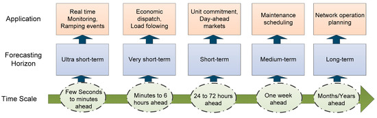
Figure 1.
Forecasting applications and their associated time scales and forecast horizons.
In a power system, day-ahead SI forecasting is essential for power system operations and day-ahead market (DAM). Accurate forecasting in unit commitment and economic dispatch provides an improved and economically efficient operation. In addition, accurate forecasting leads to better utilization of PV power and hence, results in less curtailment, reduced uncertainty in power system operations, and minimized overall operating cost. The study on the impact of the day-ahead solar energy forecasting for an independent system operator in New England (ISO-NE) on system operation and overall operating cost is presented in [14].
Day-ahead forecasting is also important to deal with the management of the operating reserve [15]. In [16], the analysis on improved SI forecasting is performed in order to see the effects on flexibility reserves while dealing with imbalanced markets. Results have shown that better forecasting leads to a reduction in flexibility reserves. Likewise, in [17] for the improved day-ahead SI forecast, authors have reported a reduction in spinning reserve requirements for various system operators and utilities. For a concentrated solar-thermal (CST) plant in Australia, [18] shows significant economic benefit for six months of operation considering the improvement in short-term SI forecasting.
In the case of DAM, the bids are performed considering day-ahead forecasting. Therefore, a highly accurate prediction for PV is essential. In [19], the analysis for day-ahead forecasting for PVs in the Spanish electricity market is provided in order to see the economic performance for various forecasting models. Similarly, in [20], the significance of accurate forecasting for solar energy is shown in the context of German electricity market conditions. Their analysis concludes that the improved forecast accuracy reduces the financial risks however, it is also related to the market prices. DAM operation considering over-forecast and under-forecast of the PV power with the effect of locational marginal prices (LMP) and the real-time market is analyzed for California [21].
In the proposed study, an improved forecasting model is presented using a hybrid approach with a deep recurrent neural network based on long short-term memory (LSTM-RNN). A clustering method is first used to classify the daily weather condition as either sunny or cloudy. Then, the LSTM-RNN model is used to predict the SI for both types of days. Clustering enables the identification of similar patterns for SI of each day type that leads to the advantage of realizing better accuracy. As the LSTM-RNN model learn the uncertainty and variability for each type of cluster separately, it allows fitting the curve with more accuracy.
The remainder of this paper is organized as follows. The related work is presented in Section 2; the methodology of the proposed hybrid LSTMM-RNN approach for SI is explained in Section 3; implementation details for the proposed method are presented in Section 4; the results are presented and discussed in Section 5, and the conclusions are summarized in Section 6.
2. Related Work
Several methods for forecasting the SI have been proposed in the literature, and these can be broadly divided into two prediction modeling categories, namely physical modeling and data-driven modeling. In a physical model, numerical weather prediction (NWP) is used for forecasting tasks by using complex mathematical equations [22,23]. The NWP method gives a good performance in stable weather conditions. However, it has limitations for cloudy weather. The coarse resolution puts a limitation to acquire the information related to the clouds [12]. In a data-driven approach, historical data are used that may or may not contain external weather parameters (temperature, humidity, clearness index, etc.) with SI. The data-driven models are further categorized into two sub-types, namely nonlinear autoregressive (NAR) models and nonlinear autoregressive with exogenous (NARX) models. The first of these uses the endogenous input (i.e., the SI) as the prediction parameter, while the latter includes the exogenous parameters such as temperature, humidity, and clearness index, along with the endogenous parameter (SI). Within the NAR and NARX categories, the data-driven models are further categorized into statistical models, artificial intelligence (AI)-based models, and hybrid models.
The statistical models used for SI forecasting are mainly based on autoregressive (AR) methods. These methods include the autoregressive moving average (ARMA), the ARMA model with exogenous variables (ARMAX) and the autoregressive integrated moving average (ARIMA) [24]. Further studies related to statistical models are available in [25,26,27,28,29,30,31,32].
The AI-based models perform better for the SI prediction as compared to conventional statistical models. Among the AI models, machine learning models have the potential to address the nonlinear relationship between input and output for prediction tasks. Machine learning models include support vector machine (SVM), the feed-forward neural network (FFNN), and the adaptive fuzzy neural network (AFNN), and so on. SVM has been used to predict the solar insolation from three years of data [33]. In another study, the daily solar irradiance was forecast for three locations in China using seven SVM models based on sunshine duration as the input [34]. The findings indicated better results for the first SVM model that shows the lowest error in the winter season as compared to other seasons. For interested readers, a comprehensive review related to the SVM based forecasting of SI and wind is presented in [35]. In addition, the FFNN approach has been used to forecast the daily SI in France using 19 years of data. The results were compared with those of other statistical and machine learning models such as AR models, Markov chains, Bayesian inference, and the k-nearest neighbor (KNN). The results indicated that the FFNN provided the best performance [36]. In another study, the FFNN approach has also been used to forecast the daily SI, based on the NAR and NARX models along with a multi-output FFNN architecture to indicate that the NARX and multi-output model provided the best performance accuracy [37]. Additional studies related to use of FFNN for predicting solar irradiance are available [38,39,40,41].
The accessibility to large quantities of data (“big data”) and the potential for training and strong generalization has attracted recent attention towards deep learning as a promising branch of AI. This approach has been widely implemented in pattern recognition, image processing, detection, classification, and forecasting applications. A deep learning network consists of multiple hidden layers that are used to learn data patterns. For SI forecasting, deep learning technologies such as the recurrent neural network (RNN), the long short term memory (LSTM), the wavelet neural network (WNN), the deep belief network (DBN), the multilayer restricted Boltzmann machine (MRBM), the convolutional neural network (CNN), and the deep neural network (DNN) are used in the literature [42]. Among these, LSTM-RNN is used to predict the SI with better accuracy. For instance, a comparative study of LSTM for predicting next-day SI has shown that the LSTM outperforms many alternative models (including the FFNN) by a substantial margin [43]. Similarly, the LSTM- RNN model with exogenous inputs has been applied and compared favorably with the FFNN [44]. Meanwhile, another study used the LSTM network to predict SI and compared the results with those obtained using the CNN, RNN, and FFNN models to demonstrate that the LSTM shows the best performance [45].
To outperform the typical deep learning methods in forecasting applications, hybrid models are presented in the literature [12]. In the hybrid approach, various models are combined to perform forecasting. For instance, one method can be used for classification (e.g., weather classification [46]) or data decomposition (e.g., wavelet decomposition [47]). While the other method is used for forecasting the main feature. Several studies have indicated that the hybrid approach has shown better performance than the single method Several studies have indicated that the hybrid approach has shown better performance than the single method [48,49,50,51]. A comprehensive review on hybrid models for solar energy forecasting is presented in [10]. In this study, k-means clustering is used for weather classification and LSTM-RNN for forecasting the SI. Classification of the days using the clustering method groups the days into similar weather types that may have similar SI patterns. The clustered data is fed to the separate forecasting models at the training stage to train on similar patterns, which allow fitting the data with more accuracy for each model and hence, improving the overall accuracy. For example, k-means clustering has been used for weather classification in combination with SVM for enhanced accuracy in [52]. The results show that the accuracy is improved for sunny days and cloudy days with RMSE of 49.26 W/m2 and 57.87 W/m2, respectively. However, partially cloudy days show the RMSE of 62.7 W/m2. While overall RMSE for non-clustered data is reported as 58.72 W/m2. In [46], a classification-based hybrid model is presented. Results have shown that the classification technique enhances forecasting accuracy. Random forest (RF) performs well for cloudy days while SVM for Sunny days with NRMSE of 41.40% and 8.88%, respectively. In another study [53], an average daily SI and clear sky model was considered for classification in combination with the FFNN for prediction to provide improved performance. In this study, k-means clustering is used for weather classification and LSTM-RNN for forecasting the SI.
Classification of the days using the clustering method groups the days into similar weather types that may have similar SI patterns. The clustered data is fed to the separate forecasting models at the training stage to train on similar patterns, which allow fitting the data with more accuracy for each model and hence, improving the overall accuracy. For example, k-means clustering has been used for weather classification in combination with SVM for enhanced accuracy in [52]. The results show that the accuracy is improved for sunny days and cloudy days with RMSE of 49.26 W/m2 and 57.87 W/m2, respectively. However, partially cloudy days show the RMSE of 62.7 W/m2. While overall RMSE for non-clustered data is reported as 58.72 W/m2. In [46], a classification-based hybrid model is presented. Results have shown that the classification technique enhances forecasting accuracy. Random forest (RF) performs well for cloudy days while SVM for Sunny days with NRMSE of 41.40% and 8.88%, respectively. In another study [53], an average daily SI and clear sky model was considered for classification in combination with the FFNN for prediction to provide improved performance. However, the classification of the day as sunny or cloudy based on the daily average may not be sufficiently accurate. Generally, a lesser amount of sunshine in the winter will lead to a low average. Therefore, it is more likely the day being classified as cloudy. Nevertheless, for the clear-sky model, it is more reasonable to classify the day as either sunny or cloudy.
As discussed above, in several studies, LSTM-RNN has shown better performance among other deep learning models for SI forecasting. Therefore, this study is aiming to combine the LSTM-RNN with weather classification to form a hybrid system due to its advantage to achieve high accuracy. In the present paper, a hybrid model is proposed that consists of k-means clustering and an LSTM-RNN network. First, the day types are classified using the k-means clustering and then, LSTM-RNN models are trained for each cluster of the day type. The classification is performed based on the clearness index using k-means clustering. To train the model for each day type, exogenous inputs are used. The results of the proposed hybrid LSTM-RNN approach are compared with those obtained using empirical methods such as the hybrid FFNN and the hybrid SVM and conventional LSTM-RNN (without weather classification). In brief, the present study makes the following contributions:
- A hybrid LSTM-RNN approach is proposed. In the first stage, the datasets of three locations are classified into cloudy and sunny days via k-means clustering. The LSTM-RNN model is then trained for each day type in the second stage using exogenous inputs.
- A comparative study with other models (including the SVM, the FFNN, and persistence models) is provided for three datasets. For a fair comparison, these models are also trained after the classification task. In addition, the proposed model is compared with the conventional LSTM-RNN model, i.e., generic model without weather classification.
3. Proposed Method
In this section, a hybrid LSTM-RNN model is presented to forecast the day-ahead SI. It uses a classification method along with the LSTM-RNN model to maximize the advantage in terms of achieving better accuracy. After classification, the days are clustered into similar weather types. Therefore, the SI of similar patterns are sorted and the models learn these patterns accordingly for each type of day (sunny day and cloudy day). Classification enables the forecasting models to learn the variability and uncertainty for each day type separately. This helps lower the complexity and difficulty of data fitting, thereby improving the forecasting accuracy. Figure 2 shows the example of sunny and cloudy days, plotted with the corresponding extraterrestrial irradiance.

Figure 2.
Example of (a) a sunny day and (b) a cloudy day for Golden, Colorado (USA).
The proposed hybrid model for SI forecasting consists of the following five steps and the overall flow of the proposed model is shown in Figure 3.
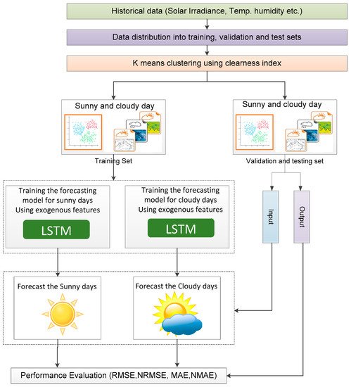
Figure 3.
The proposed hybrid approach for SI forecasting.
Step 1: historical data are collected from the weather stations. These data include the SI along with the other weather parameters such as humidity, dew point temperature, etc., that have been previously used as exogenous features in forecasting models.
Step 2: the clearness index for each day is then defined as the ratio of the SI at the surface of the Earth (I) to the extraterrestrial irradiation (I0), as shown in Equation (1): [54]
Thus, the clearness index varies between 0 and 1, where 0 means 100% overcast and 1 indicates clear weather. The values for SI and extraterrestrial irradiation are taken as a daily average to calculate the clearness index. The clearness index can be computed using the SI from weather stations, which is obtained using NWP methods and is available for several days [55]. In this way, we can classify the next day as a cloudy or sunny day. The accuracy might not be high for such NWP methods. However, these can be used to classify the day as a cloudy or sunny day by averaging the predicted SI for a day.
Step 3: k-means clustering is used to divide the data into sunny and cloudy days based on the clearness index. In addition, the classification based on two parameters is also performed to see the effects on accuracy. For this purpose, the percentage of cloud covers with a clearness index is used to classify the day.
Step 4: the forecasting model is then trained for sunny and cloudy days. For comparison, three models (LSTM, FFNN and SVM) are trained for both days. Each forecasting model is fed with only exogenous features in order to train each model for both types of days.
Step 5: Finally, the results are tested and validated for each type of day via various performance matrices.
As noted in Step 4, although the prime focus of this study is to use the LSTM forecasting model with the clustering approach using exogenous features, the results are compared with those obtained using the other forecasting models (i.e., FFFN and SVM). In addition, the k-means clustering is used with the FFNN and SVM models in order to provide a fair comparison. Each of these models is described and discussed in the following subsections in order to provide a better intuition regarding their mechanisms.
Detailed LSTM-RNN Architecture with k-Means Clustering
The primary focus of the present study is to train the LSTM-RNN network using the results of classification. In this approach, SI data were fed into the k-means clustering algorithm. The clearness index was calculated from the extraterrestrial irradiance and surface solar irradiance via Equation (1). The days were accordingly classified as sunny or cloudy. The results were then used to train the LSTM-RNN network for each day type from the associated data. The detailed architecture of the proposed approach is shown in Figure 4.

Figure 4.
The LSTM-RNN architecture with k-means clustering.
After classification, the LSTM network is trained for each day type. From Figure 4, dashed boxes represent the training examples that input to the LSTM network. The feature dimensions for M number of training examples include exogenous and categorical features for each example, where t presents the time steps, which are 24 h in day-ahead forecasting for each training example.
The network consists of various layers, including the input layer, several LSTM-based hidden layers, the fully connected layer, and the output layer. The inclusion of more than one LSTM-based layer increases the depth of the network and helps it to learn the temporal dependencies associated with the relevant time steps. The fully connected layer and output layer are used to output the predicted result.
From the input layer, the first-time step of the training example is fed to the first LSTM unit. The initial state of the network is also fed into the LSTM unit in order to compute the first output . It updates cell state as well. At time step t, the corresponding LSTM unit takes the current state of the network () and time step from training example to generate the output and update the cell state . After passing the examples from the network, final outputs for day-ahead SI are generated as .
4. Implementation Details
The experimental description for the proposed methodology is presented in this Section. Separate subsections are dedicated to dataset description, data division, feature selection, and hyperparameter optimization.
4.1. Dataset Description
To demonstrate the diversity of the proposed study, datasets from three locations in the USA, Germany, and Switzerland are included. Information about the sizes of the dataset, latitude and longitude for all locations are mentioned in Table 1.These datasets were recorded from the following weather stations: The Solar Radiation Research Laboratory (SRRL) in Golden, Colorado (USA) [56], the weather station at the Max Planck Institute of Biochemistry (MPIB) in Jena (Germany) [57], and the weather station in Basel, Switzerland [58].

Table 1.
The location co-ordinates and dataset size.
These datasets include the other parameters to be considered along with SI for the present study, including the dew point temperature, the relative humidity, the dry bulb temperature, cloud covers, wind speed, etc. These are taken as the exogenous features. These obtained input features are the measured values. For the proposed model, these are assumed as the perfectly forecasted values because these exogenous features are used as the forecasted metrological data for the next day as inputs to predict the SI.
4.2. Data Division
In many studies, the datasets are divided into training and testing sets only. In the present study, the datasets are divided into training, validation, and test sets. The distributions of the datasets are detailed in Table 2. The training set is used to train the proposed model. The validation set is used to tune the hyperparameters, regularization, and feature selection process. Finally, the test set is used to evaluate the performance of the model. Results for validation data sets are reported in Appendix B. Performance of the proposed model is evaluated and discussed using test sets in Section 4.
Table 2.
Dataset distribution.
4.3. Feature Selection
Feature selection is crucial to the performance of the forecasting algorithm [59]. In the present study, the SI was selected for the unsupervised k-means clustering of the datasets in order to classify the days as either sunny or cloudy day. For the LSTM-RNN, model external parameters (exogenous input parameters) are selected to train it for clustered data. The correlation of the external parameters with the SI was calculated using Pearson’s correlation coefficient (PCC). It enables to see the relevancy of the external parameters towards the SI. The PCC ranges from −1 to +1, with a value close to +1 indicating a higher correlation and values approaching −1 indicating a negative or inverse relationship. For example, relative humidity has a negative value that shows an inverse relationship with SI. In this case, if relative humidity goes high, SI goes down and vice versa. PCC of external parameters with SI is shown in Figure 5. At the x-axis, the locations are mentioned whereas, the y-axis presents the variables including SI and other external parameters. Each box shows the PCC value for the variable with SI.
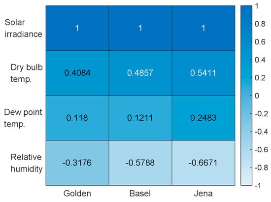
Figure 5.
The PCC of each variable with the SI for all the dataset locations.
Provided two variables (X,S), the formula for calculating PCC is given below in Equation (2):
where μ and σ are the mean and standard deviation of the variables (X,S), and N is the number of observations in each variable.
For the proposed study, an error evaluation approach was used to select the suitable features among the exogenous features, i.e., listed in Section 4.1. This approach is known as the wrapper approach [60]. According to this approach, errors for all the possible variable subsets are evaluated using evaluation metrics such as RMSE, in this study. We evaluated the results for various combinations of the variables (exogenous inputs) and find out the combination that showed the minimum error. The error was evaluated using training and validation sets. The features’ selection method indicated that the dry-bulb temperature, the dew point temperature and the relative humidity were the best choices for the analysis.
For features selection, various other methods are reported that are related to correlation methods. Nevertheless, the wrapper approach is used in this study. Using other correlation methods for feature selection, may not give us good performance because the correlation of a feature can be irrelevant by itself. However, it can provide better performance improvement when combining with other features.
To further highlight the improved performance, additional categorical features are introduced to this methodology, namely: the hours of the day (1–24) and the months of the year (1–12).
4.4. Hyperparameter Tuning
As well as depending on the feature selection process described in Section 4.3, the performance of the forecasting model is highly dependent on the selection of the hyperparameters that are used for tuning the learning rate. Moreover, the hyperparameter selection also affects the computation and memory factors. Therefore, optimization of the hyperparameters is always a point of debate among researchers. Nevertheless, some rules have been defined by scientists and researchers for setting the values. In the present study, the following hyperparameters were considered for tuning the model: feature scaling, learning rate, optimization solver, number of epochs, dropout rate, number of hidden units, and number of hidden layers.
As the computation significantly depends on the learning rate, this is the most important hyperparameter. For the optimization solver, the adaptive moment estimation (ADAM) [61], stochastic gradient descent with momentum (SGDM) [62], and RMSprop [63,64] algorithms were tested, and SGDM was found to be the best solver. For hyperparameter optimization, search space is defined based on the trial and error method. Based on the defined search space, the hyperparameters were finally optimized. Table 3 shows the hyperparameters with the chosen optimal value for the LSTM-RNN model from the search space. In addition, hyperparameters were optimized using only the Golden dataset and applied these same parameters to other datasets. It avoids the over tuning of the model.
Table 3.
Hyperparameter optimization.
The number of hidden layers was optimized as 3 and the hidden units were optimized as 24. Feature scaling showed the best results with a standard scaler method. The dropout rate was set to 0.1, which also works to avoid the overfitting problem. Finally, the number of epochs was tuned to 1500.
By contrast, the hyperparameters used for the FFNN network were the same as in a previous study [44], i.e., the learning rate was 0.001, the number of hidden units was 10, and 2 hidden layers were set. Full batch gradient descent was used, along with L2 regularization, standard scalar, and 1000 epochs.
For the SVM algorithm, standard feature scaling and a gaussian kernel were used with a sequential minimal optimization (SMO).
4.5. Performance Evaluation
The performance was evaluated using four indicators that are widely used in the literature to evaluate the performance of forecasting models. These are: the root mean square error (RMSE), the normalized root mean square error (NRMSE), the mean absolute error (MAE), and the normalized mean absolute error (NMAE), as defined by Equations (3)–(6) [65,66,67]:
where and are the actual and predicted points, and N is the total number of samples. Thus, normalization of the RMSE and MAE is performed using the min-max method.
5. Results and Discussion
The results obtained using the proposed methodology and four comparison models (including the persistence model) for three locations are presented in this Section. Test sets of all the locations are used to perform the performance evaluation for all the models. Validation sets are used for the validation of the models. Results for the validation are reported in Appendix B. The simulations were performed on a desktop computer using the Windows 10 operating system (OS) with an Intel i7 processor and 16 GB RAM. The classification is performed using k-means clustering.
5.1. Clustering with One Parameter
The results for sunny and cloudy days at each location are indicated in Figure 6, and the corresponding centroid values are listed in Table 4. For example, the Golden (Colorado) location has sunny and cloudy days with centroid values of 0.69 and 0.38, respectively. If the clearness index is high, then the day is more likely to be sunny and vice versa. After classifying the days as sunny or cloudy based on the centroid value at each location, the LSTM-RNN, FFNN, SVM, and persistence models are each trained for cloudy and sunny days.

Figure 6.
The classification of days via k-means clustering for the study locations.
Table 4.
The centroid values for sunny and cloudy days at the study locations.
The results obtained using the various models are presented and evaluated according to their RMSE, NRMSE, MAE, and NMAE values in Table 5. In addition, the average NRMSEs of the four models for the three geographical locations are indicated by the bar charts in Figure 7. Thus, it can be seen that the proposed LSTM model gives the best performance for all three locations, followed by the FFNN and SVM models, while the persistence model gives the least accurate forecasting results.
Table 5.
The obtained results for the proposed hybrid model and other models.

Figure 7.
The average NRMSE at the three locations for each model.
In detail, the LSTM provides minimum and maximum average NRMSEs 4.15 and 5.93%, respectively, over both types of days. While the average NMAE error percentage is ~2%. With respect to the three locations, all four models give their best performances for the data from Golden (Colorado). Overall, the proposed model gives a better performance on sunny days as compared to cloudy days. In addition, the SVM and FFNN giving closely comparable performances and low deviations. Therefore, since more time is required to train the FFNN than the SVM, the computational burden at the training stage can be reduced by selecting the SVM rather than the FFNN.
The measured SI and the corresponding values for cloudy and sunny days predicted by the proposed and comparison models at the three locations are plotted graphically in Figure 8. The results for sunny days are presented in the left-hand column of the figure, while those for cloudy days are presented in the right-hand column. Thus, it can be seen that the persistence model gives the worst performance for both day types, while the LSTM gives better results than all other models. Comparatively, the results for cloudy days are less accurate than those for sunny days.

Figure 8.
Graphical comparison of the measured and predicted SI values for (a) sunny and (b) cloudy days at (top to bottom) Golden, Basel, and Jena.
The results of the proposed model for the three locations are also compared with those obtained using the conventional LSTM model in Table 6 and Figure 9. The conventional LSTM-RNN model is trained, validated, and tested for the whole dataset without classifying the days into sunny and cloudy. Therefore, it can be referred to as the all-sky model. As expected, these results indicate that the hybrid LSTM provides the better performance, with a minimum error of 4.15% for the Golden (Colorado) prediction and a maximum error of 5.93% for the Basel prediction. By contrast, the conventional LSTM gives errors of 5.56 and 7.98% at Golden and Basel, respectively. This is because the proposed approach learns the SI pattern well and helps predict the SI more accurately as compared to the conventional method.
Table 6.
A performance comparison of the hybrid and conventional LSTM models.
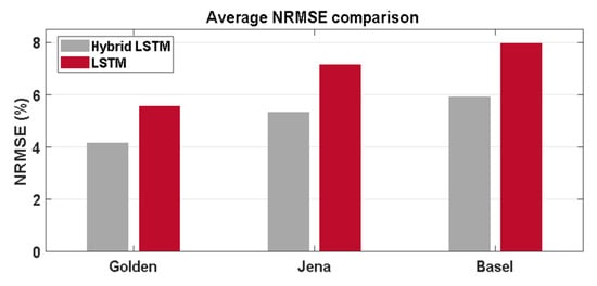
Figure 9.
Bar charts comparing the average NRMSEs for the hybrid and Conventional LSTM models.
Scatter plots of the measured SI values at each location against those predicted by the proposed hybrid LSTM model are presented in Figure 10 for sunny (left-hand column) and cloudy (right-hand column) days. The goodness of fit to a straight line is also indicated, with points close to the blue line indicating more accurate predictions and points far from the line indicating less accurate prediction. Thus, the proposed model is seen to accurately predict the data measured at Golden (Colorado) for both cloudy and sunny days, whereas the predictions at other sites are less accurate for cloudy days than for sunny days.

Figure 10.
Scatter plots of the measured SI value at each location against that predicted by the hybrid LSTM-RNN model for (a) sunny and (b) cloudy days.
5.2. Clustering with Two Parameters
So far, the analyses have been performed for one dimension k-means clustering for the classification. In previous studies such as [45,52], two variables are used to classify the day. Therefore, we have performed classification with two parameters and compare the performance of the forecasting with a single parameter classification-based model. To see the effects of two parameters on classification, one site is considered for further analysis. For this purpose, the cloud covers are considered with a clearness index to define a sunny and cloudy day. If the percentage of the cloud covers is high and the clearness index is low, then the day is more likely to be classified as cloudy. Figure 11 shows the classification for Golden, Colorado (USA) with two parameters.

Figure 11.
Classification with two parameters for Golden.
The results for various forecasting techniques considering both sunny and cloudy days are presented in Table 7. Results show the supremacy of LSTM among other models as expected. Average NRMSE for LSTM, FFNN, SVM and persistence models are recorded as 4.65%, 5.46%, 5.76% and 11.58%, respectively. Errors for this approach are closely comparable with the former classification approach, however, performance is not improved. Therefore, the classification using one parameter is suitable for forecasting with the advantage of better accuracy and less computation burden as more computation time is required for a classification task that uses two parameters.
Table 7.
Results for the proposed and other models with two parameters clustering for Golden.
Overall, the proposed model is showing better performance for forecasting the SI, however, it has some limitations for a practical system. As in this study, inputs are obtained from the weather stations that are measured values and are assumed as the perfectly forecasted values for the proposed approach. However, in a real system, these exogenous features are used as the forecasted metrological data for the next day to predict the SI. Therefore, the accuracy of the SI prediction may be affected by a forecasted error of the meteorological data. This is the limitation of the data-driven forecasting approach that uses exogenous features as inputs.
Another limitation is related to the data availability. We trained the model using several years’ measured data. However, in practice, it might be difficult to obtained measured data of several years to train the model, specifically, for a new site. The proposed solution to the limitation is the generalization of the model for SI forecasting [68]. The model can be generalized using the data from the nearby weather station and the use for the new site. The performance of the generalized model may vary however, but can be improved with time. The model can be trained continuously using upcoming data for a particular site.
6. Conclusions
In this paper, a hybrid LSTM-RNN framework for forecasting the SI was proposed and compared with the hybrid approach with FFNN and SVM. K-means clustering was used to classify the days as either sunny or cloudy, then the LSTM-RNN model was used to forecast the SI, and exogenous features were used to train the model. The proposed model was shown to provide the best performance for all three study locations (Golden, Colorado (USA), Jena (Germany), and Basel (Switzerland)) followed by the FFNN and SVM models. In detail, the hybrid LSTM provided maximum and minimum average NRMSEs 4.15% and 5.93% over both types of the day at Golden and Basel, respectively. In terms of the NMAE, the average error percentage was around 2% for both types of day. Overall, the proposed model provided better performance on sunny days than on cloudy days. Furthermore, the hybrid LSTM model exhibited less error than the conventional LSTM model, as indicated by the maximum NRMSEs of 4.15% and 5.56%, respectively.
In addition, the proposed approach is tested for classification considering two parameters (clearness index and cloud covers). Results have shown no improvement in the forecasting as compared to the former way of clustering. Therefore, using one dimension k-means clustering should be significant to use with the advantages of better performance and less computational burden. Finally, it is concluded that as compared to other methods, the proposed hybrid approach to day-ahead SI forecasting can be a more suitable option for power-system applications such as unit commitment, economic dispatch, and other day-ahead market operations.
In future works, we are aiming to perform the analysis and comparison on the effect of errors from forecasted meteorological data. More analysis will be performed on k-means clustering with various combinations of the parameters to see the effect of the classification on the overall model performance. Furthermore, generalization of the proposed model will be performed to make the model more suitable for practical use.
Author Contributions
Conceptualization, R.Z., B.H.V., M.H. and I.-Y.C.; investigation, R.Z.; methodology, R.Z. and B.H.V.; formal analysis, R.Z. and I.-Y.C.; resources, R.Z., M.H. and I.-Y.C.; writing—original draft preparation, R.Z.; writing—review and editing, R.Z. and I.-Y.C.; supervision, I.-Y.C.; All authors have read and agreed to the published version of the manuscript.
Funding
This research was supported by the National Research Foundation of Korea (NRF) grant funded by the Korea government (MSIT) (No. 2019R1A2C1003880) and the Korea Institute of Energy Technology Evaluation and Planning (KETEP) grant funded by the Korea government (MOTIE) (2019371010006B).
Institutional Review Board Statement
Not applicable.
Informed Consent Statement
Not applicable.
Data Availability Statement
Not applicable.
Conflicts of Interest
The authors declare no conflict of interest.
Appendix A. Theoretical Overview
Appendix A.1. The K-Means Clustering Algorithm
K-means clustering is an unsupervised machine learning algorithm used to allocate data points into groups or clusters by identifying the mean distance between data points [69]. This process is then iterated to provide more precise classifications over the course of time. In k-means clustering, the basic concept is to choose a number (k) of centroids for each cluster. Since different positions of centroids produce distinct results, it is possible to place the centroids strategically. The better option, however, is to position them at large distances from each other. After defining the centroids, a point is taken from the dataset and linked to the closest centroid. This process is first performed for all the points to generate an initial grouping, then the k new cluster centroids are calculated accordingly. Based on the k new centroids, new associations are then made between the same dataset points and the closest new centroids. Thus, the centroids change their positions iteratively until no further adjustments can be made (i.e., the problem has converged to one solution). In brief, the algorithm minimizes an objective function (a squared error function in the present case) to form an association between centroids and dataset points. The objective function is given by Equation (2) [69]:
where is a chosen distance measure between data-point and the cluster center as an indicator of the distance of the n data points from their respective cluster centers.
Appendix A.2. The Support Vector Machine (SVM)
The SVM is a machine learning method that was introduced by Cortes and Vapnik to perform classification and regression tasks [70]. To predict time series data, the SVM performs a regression or support vector regression (SVR).
The dataset for training the SVR model is formed in the same way as for other models, with input and output pairs the regression problem is then given as the map in Equation (A2):
where is the weight factor and b is the bias value. To find the flat , it is necessary to minimize the norm value () of the weighting factors via Equation (A3):
This is subject to the inequality in Equation (A4):
which indicates that the function provides an accurate approximation within the margin of ±ε. However, it not always possible to maintain a tight margin. To solve this problem, points that lie outside the margin are dealt with by the introduction of slack variables . The objective function then takes the form of Equation (A5):
which is subject to the in Equalities (A6) and (A7):
The constant C is the controller for the slack variables and has a value greater than zero. This defines the amount of deviation of the slack variables .
Appendix A.3. The Feed-Forward Neural Network (FFNN)
The FFNN is used to map input and output to provide a better approximation of the function , where and w and b are the weights and bias vectors, respectively. These values are adjusted via the learning process [71]. Typically, the FFNN consists of an input layer, one or more hidden layers, and an output layer. The inputs are taken from the input layer to the hidden layer, and then the calculated values are transferred to the output layer. At the output layer, a specific type of calculation is performed depending upon whether the task is a classification or regression task. This depends on the activation function and the data orientation. The simplified calculation for the FFNN is described by Equations (A8)–(A11) below.
There are n input signals (or nodes) in the input layer, M hidden units in the hidden layer, and k output signals in the output layer. This allows the construction of M linear combinations of input variables x1,…, xn as in Equations (A8) and (A9):
where is the index and M the total number of linear combinations of input variables (i.e., ), and are the weights and biases, and is the linear combination of the weighted sum. The value is then passed to the activation function that applies a transformation (e.g., tanh, logistic sigmoid, rectified linear unit (Relu), etc.) to the output (zj) of the hidden layer. This process is then repeated for the output layer, as in Equations (A10) and (A11):
where (K being the total number of outputs), and and are the weights and biases for the output layer from the hidden layer. The output unit activations are then finally transformed via an activation function to produce a set of network outputs yk.
To learn the weights and bias values, the FFNN employs backpropagation algorithms to reduce the error between the predicted and actual output values in order to provide an accurate prediction.
Appendix A.4. The Long Term Short Term Memory-Based Recurrent Neural Network (LSTM-RNN)
Although the FFNN model discussed in the previous subsection does not use the information from the previous time steps to learn the equations, this information has significant value in improving the performance of a prediction task. To overcome this problem, RNN is introduced into time series forecasting. The RNN uses the information from the output of the previous step to predict the next time step. However, because this is an iterative process, the retention of information for a long time may lead to a vanishing gradient problem that results in worse predictions. To solve this problem, LSTM-based RNN is used to store the relevant information from the previous time steps and discard any information that is not needed. These tasks are performed using different gate functionalities in the LSTM cell.
The LSTM was developed in 1997 by Hochreiter and Schmidhuber [72]. In the LSTM-RNN network, hidden RNN layers are replaced by the LSTM cells. As shown in Figure A1, each cell consists of various gates that can manage the inputs and outputs, including an input gate, a forget gate, a cell state, and an output gate. The LSTM cells also contain a tanh block, a sigmoid block, and a multiplication function. The input gate is used to store new information in the memory, while the forget gate is responsible for discarding the previously stored information when it is activated. Finally, activation of the output gate allows the propagation of the latest cell output to the ultimate state. The function of the sigmoid block is to generate values between 0 and 1 to indicate what percentage of each component should be allowed. The tanh block creates a new vector to be added to the state, and the cell state is accordingly reorganized depending on the outputs formed by the gates. Mathematically, LSTM cells can be represented by the Equations (A12)–(A16): [73]
where σ is the sigmoid, i, f, o and c are the input gate, forget gate, output gate, and cell gate, respectively, h is the hidden vector that defines the (identical) size of each gate, and W is the weight matrix.

Figure A1.
The LSTM cell [73].
Appendix B
Table A1.
The obtained results for the proposed hybrid model and other models for the training set.
Table A1.
The obtained results for the proposed hybrid model and other models for the training set.
| Location | Model | RMSE (W/m2) | NRMSE (%) | MAE (W/m2) | NMAE (%) | ||||||||
|---|---|---|---|---|---|---|---|---|---|---|---|---|---|
| Sunny | Cloudy | Avg. | Sunny | Cloudy | Avg. | Sunny | Cloudy | Avg. | Sunny | Cloudy | Avg. | ||
| Golden | LSTM | 42.31 | 46.03 | 44.17 | 3.89 | 4.58 | 4.24 | 19.53 | 15.57 | 17.55 | 1.79 | 1.55 | 1.67 |
| FFNN | 47.48 | 48.72 | 48.10 | 4.37 | 4.85 | 4.61 | 22.05 | 16.19 | 19.12 | 2.02 | 1.61 | 1.82 | |
| SVM | 56.13 | 55.58 | 55.86 | 5.16 | 5.53 | 5.35 | 27.10 | 18.22 | 22.66 | 2.49 | 1.81 | 2.15 | |
| Pers. | 97.58 | 106.91 | 102.25 | 8.98 | 10.64 | 9.81 | 42.06 | 35.02 | 38.54 | 3.87 | 3.48 | 3.68 | |
| Jena | LSTM | 47.27 | 50.90 | 49.09 | 4.97 | 5.71 | 5.34 | 20.45 | 20.52 | 20.49 | 2.30 | 2.36 | 2.33 |
| FFNN | 55.45 | 52.17 | 53.81 | 5.83 | 5.85 | 5.84 | 25.04 | 22.37 | 23.71 | 2.63 | 2.51 | 2.57 | |
| SVM | 57.89 | 56.92 | 57.41 | 6.09 | 6.38 | 6.24 | 24.66 | 21.93 | 23.30 | 2.59 | 2.46 | 2.53 | |
| Pers. | 81.31 | 81.11 | 81.21 | 8.56 | 9.10 | 8.83 | 32.81 | 32.37 | 32.59 | 3.45 | 3.63 | 3.54 | |
| Basel | LSTM | 45.67 | 54.14 | 49.91 | 5.29 | 6.45 | 5.87 | 22.79 | 18.94 | 20.87 | 2.58 | 2.25 | 2.42 |
| FFNN | 53.67 | 47.71 | 50.69 | 6.08 | 5.68 | 5.88 | 25.40 | 17.73 | 21.57 | 2.88 | 2.11 | 2.50 | |
| SVM | 55.19 | 52.73 | 53.96 | 6.25 | 6.28 | 6.27 | 24.85 | 18.99 | 21.92 | 2.81 | 2.26 | 2.54 | |
| Pers. | 72.63 | 81.00 | 76.82 | 8.23 | 9.95 | 9.09 | 28.91 | 28.13 | 28.52 | 3.27 | 3.35 | 3.31 | |
References
- Gielen, D.; Gorini, R.; Wagner, N.; Leme, R.; Gutierrez, L.; Prakash, G.; Asmelash, E.; Janeiro, L.; Gallina, G.; Vale, G. Global Energy Transformation: A Roadmap to 2050; IRENA: Abu Dhabi, United Arab Emirates, 2019; pp. 1–51. [Google Scholar]
- Dyl, K. Annual Energy Outlook 2018 with Projections to 2050. Annu. Energy Outlook 2018, 44, 1–64. [Google Scholar]
- Yanar, N.; Choi, H. Energy Perspectives of Korea (Republic of) with a General Outlook on Renewable Energy. IGLUS Q. 2019, 4, 4–8. [Google Scholar]
- Yang, X.J.; Hu, H.; Tan, T.; Li, J. China’s renewable energy goals by 2050. Environ. Dev. 2016, 20, 83–90. [Google Scholar] [CrossRef]
- Hansen, J.; Kharecha, P.; Sato, M.; Masson-Delmotte, V.; Ackerman, F.; Beerling, D.J.; Hearty, P.J.; Hoegh-Guldberg, O.; Hsu, S.-L.; Parmesan, C. Assessing “dangerous climate change”: Required reduction of carbon emissions to protect young people, future generations and nature. PLoS ONE 2013, 8, e81648. [Google Scholar]
- Wang, K.; Qi, X.; Liu, H. A comparison of day-ahead photovoltaic power forecasting models based on deep learning neural network. Appl. Energy 2019, 251, 113315. [Google Scholar] [CrossRef]
- Ellahi, M.; Abbas, G.; Khan, I.; Koola, P.M.; Nasir, M.; Raza, A.; Farooq, U. Recent approaches of forecasting and optimal economic dispatch to overcome intermittency of wind and photovoltaic (PV) systems: A review. Energies 2019, 12, 4392. [Google Scholar] [CrossRef]
- Clack, C.T. Modeling solar irradiance and solar PV power output to create a resource assessment using linear multiple multivariate regression. J. Appl. Meteorol. Climatol. 2017, 56, 109–125. [Google Scholar] [CrossRef]
- Alzahrani, A.; Shamsi, P.; Dagli, C.; Ferdowsi, M. Solar irradiance forecasting using deep neural networks. Procedia Comput. Sci. 2017, 114, 304–313. [Google Scholar] [CrossRef]
- Guermoui, M.; Melgani, F.; Gairaa, K.; Mekhalfi, M.L. A comprehensive review of hybrid models for solar radiation forecasting. J. Clean. Prod. 2020, 258, 120357. [Google Scholar] [CrossRef]
- Sharma, A.; Kakkar, A. Forecasting daily global solar irradiance generation using machine learning. Renew. Sustain. Energy Rev. 2018, 82, 2254–2269. [Google Scholar] [CrossRef]
- Diagne, M.; David, M.; Lauret, P.; Boland, J.; Schmutz, N. Review of solar irradiance forecasting methods and a proposition for small-scale insular grids. Renew. Sustain. Energy Rev. 2013, 27, 65–76. [Google Scholar] [CrossRef]
- Giebel, G.; Kariniotakis, G. Best practice in short-term forecasting-a users guide. In Proceedings of the CD-Rom Proceedings European Wind Energy Conference, Milan, Italy, 7 May 2007. [Google Scholar]
- Martinez-Anido, C.B.; Botor, B.; Florita, A.R.; Draxl, C.; Lu, S.; Hamann, H.F.; Hodge, B.-M. The value of day-ahead solar power forecasting improvement. Sol. Energy 2016, 129, 192–203. [Google Scholar] [CrossRef]
- Ela, E.; Milligan, M.; Kirby, B. Operating Reserves and Variable Generation; National Renewable Energy Lab.(NREL): Golden, CO, USA, 2011. [Google Scholar]
- Kaur, A.; Nonnenmacher, L.; Pedro, H.T.; Coimbra, C.F. Benefits of solar forecasting for energy imbalance markets. Renew. Energy 2016, 86, 819–830. [Google Scholar] [CrossRef]
- Zhang, J.; Hodge, B.-M.; Lu, S.; Hamann, H.F.; Lehman, B.; Simmons, J.; Campos, E.; Banunarayanan, V.; Black, J.; Tedesco, J. Baseline and target values for regional and point PV power forecasts: Toward improved solar forecasting. Sol. Energy 2015, 122, 804–819. [Google Scholar] [CrossRef]
- Law, E.W.; Kay, M.; Taylor, R.A. Calculating the financial value of a concentrated solar thermal plant operated using direct normal irradiance forecasts. Sol. Energy 2016, 125, 267–281. [Google Scholar] [CrossRef]
- Antonanzas, J.; Pozo-Vázquez, D.; Fernandez-Jimenez, L.; Martinez-de-Pison, F. The value of day-ahead forecasting for photovoltaics in the Spanish electricity market. Sol. Energy 2017, 158, 140–146. [Google Scholar] [CrossRef]
- Ruhnau, O.; Hennig, P.; Madlener, R. Economic implications of enhanced forecast accuracy: The case of photovoltaic feed-in forecasts. FCN Work. Pap. 2015. [Google Scholar] [CrossRef][Green Version]
- Luoma, J.; Mathiesen, P.; Kleissl, J. Forecast value considering energy pricing in California. Appl. Energy 2014, 125, 230–237. [Google Scholar] [CrossRef]
- Pu, Z.; Kalnay, E. Numerical weather prediction basics: Models, numerical methods, and data assimilation. In Handbook of Hydro Meteorological Ensemble Forecasting; Springer: Berlin/Heidelberg, Germany, 2019; pp. 1–31. [Google Scholar]
- Hanifi, S.; Liu, X.; Lin, Z.; Lotfian, S. A critical review of wind power forecasting methods—Past, present and future. Energies 2020, 13, 3764. [Google Scholar] [CrossRef]
- Ghofrani, M.; Suherli, A. Time series and renewable energy forecasting. In Time Series Analysis and Applications; IntechOpen: London, UK, 2017; pp. 77–92. [Google Scholar]
- Boileau, E. Use of some simple statistical models in solar meteorology. Sol. Energy 1983, 30, 333–339. [Google Scholar] [CrossRef]
- Mora-Lopez, L.; Sidrach-de-Cardona, M. Multiplicative ARMA models to generate hourly series of global irradiation. Sol. Energy 1998, 63, 283–291. [Google Scholar] [CrossRef]
- Santos, J.; Pinazo, J.; Cañada, J. Methodology for generating daily clearness index index values Kt starting from the monthly average daily value t. Determining the daily sequence using stochastic models. Renew. Energy 2003, 28, 1523–1544. [Google Scholar] [CrossRef]
- Alsharif, M.H.; Younes, M.K.; Kim, J. Time series ARIMA model for prediction of daily and monthly average global solar radiation: The case study of Seoul, South Korea. Symmetry 2019, 11, 240. [Google Scholar] [CrossRef]
- Li, Y.; Su, Y.; Shu, L. An ARMAX model for forecasting the power output of a grid connected photovoltaic system. Renew. Energy 2014, 66, 78–89. [Google Scholar] [CrossRef]
- Singh, B.; Pozo, D. A guide to solar power forecasting using ARMA models. In Proceedings of the 2019 IEEE PES Innovative Smart Grid Technologies Europe (ISGT-Europe), Bucharest, Romania, 29 September–2 October 2019; pp. 1–4. [Google Scholar]
- Benmouiza, K.; Cheknane, A. Small-scale solar radiation forecasting using ARMA and nonlinear autoregressive neural network models. Theor. Appl. Climatol. 2016, 124, 945–958. [Google Scholar] [CrossRef]
- Hassan, J. ARIMA and regression models for prediction of daily and monthly clearness index. Renew. Energy 2014, 68, 421–427. [Google Scholar] [CrossRef]
- Ekici, B.B. A least squares support vector machine model for prediction of the next day solar insolation for effective use of PV systems. Measurement 2014, 50, 255–262. [Google Scholar] [CrossRef]
- Chen, J.-L.; Li, G.-S.; Wu, S.-J. Assessing the potential of support vector machine for estimating daily solar radiation using sunshine duration. Energy Convers. Manag. 2013, 75, 311–318. [Google Scholar] [CrossRef]
- Zendehboudi, A.; Baseer, M.; Saidur, R. Application of support vector machine models for forecasting solar and wind energy resources: A review. J. Clean. Prod. 2018, 199, 272–285. [Google Scholar] [CrossRef]
- Paoli, C.; Voyant, C.; Muselli, M.; Nivet, M.-L. Forecasting of preprocessed daily solar radiation time series using neural networks. Sol. Energy 2010, 84, 2146–2160. [Google Scholar] [CrossRef]
- Voyant, C.; Randimbivololona, P.; Nivet, M.L.; Paoli, C.; Muselli, M. Twenty four hours ahead global irradiation forecasting using multi-layer perceptron. Meteorol. Appl. 2014, 21, 644–655. [Google Scholar] [CrossRef]
- Amrouche, B.; Le Pivert, X. Artificial neural network based daily local forecasting for global solar radiation. Appl. Energy 2014, 130, 333–341. [Google Scholar] [CrossRef]
- Cornaro, C.; Pierro, M.; Bucci, F. Master optimization process based on neural networks ensemble for 24-h solar irradiance forecast. Sol. Energy 2015, 111, 297–312. [Google Scholar] [CrossRef]
- Leva, S.; Dolara, A.; Grimaccia, F.; Mussetta, M.; Ogliari, E. Analysis and validation of 24 hours ahead neural network forecasting of photovoltaic output power. Math. Comput. Simul. 2017, 131, 88–100. [Google Scholar] [CrossRef]
- Marquez, R.; Coimbra, C.F. Forecasting of global and direct solar irradiance using stochastic learning methods, ground experiments and the NWS database. Sol. Energy 2011, 85, 746–756. [Google Scholar] [CrossRef]
- Shamshirband, S.; Rabczuk, T.; Chau, K.-W. A Survey of Deep Learning Techniques: Application in Wind and Solar Energy Resources. IEEE Access 2019, 7, 164650–164666. [Google Scholar] [CrossRef]
- Srivastava, S.; Lessmann, S. A comparative study of LSTM neural networks in forecasting day-ahead global horizontal irradiance with satellite data. Sol. Energy 2018, 162, 232–247. [Google Scholar] [CrossRef]
- Husein, M.; Chung, I.-Y. Day-ahead solar irradiance forecasting for microgrids using a long short-term memory recurrent neural network: A deep learning approach. Energies 2019, 12, 1856. [Google Scholar] [CrossRef]
- Yu, Y.; Cao, J.; Zhu, J. An LSTM short-term solar irradiance forecasting under complicated weather conditions. IEEE Access 2019, 7, 145651–145666. [Google Scholar] [CrossRef]
- Ali-Ou-Salah, H.; Oukarfi, B.; Bahani, K.; Moujabbir, M. A New Hybrid Model for Hourly Solar Radiation Forecasting Using Daily Classification Technique and Machine Learning Algorithms. Math. Probl. Eng. 2021, 2021, 6692626. [Google Scholar] [CrossRef]
- Mandal, P.; Madhira, S.T.S.; Meng, J.; Pineda, R.L. Forecasting power output of solar photovoltaic system using wavelet transform and artificial intelligence techniques. Procedia Comput. Sci. 2012, 12, 332–337. [Google Scholar] [CrossRef]
- Cao, J.C.; Cao, S. Study of forecasting solar irradiance using neural networks with preprocessing sample data by wavelet analysis. Energy 2006, 31, 3435–3445. [Google Scholar] [CrossRef]
- Ji, W.; Chee, K.C. Prediction of hourly solar radiation using a novel hybrid model of ARMA and TDNN. Sol. Energy 2011, 85, 808–817. [Google Scholar] [CrossRef]
- Cao, J.; Lin, X. Application of the diagonal recurrent wavelet neural network to solar irradiation forecast assisted with fuzzy technique. Eng. Appl. Artif. Intell. 2008, 21, 1255–1263. [Google Scholar] [CrossRef]
- Li, S.; Ma, H.; Li, W. Typical solar radiation year construction using k-means clustering and discrete-time Markov chain. Appl. Energy 2017, 205, 720–731. [Google Scholar] [CrossRef]
- Bae, K.Y.; Jang, H.S.; Sung, D.K. Hourly solar irradiance prediction based on support vector machine and its error analysis. IEEE Trans. Power Syst. 2016, 32, 935–945. [Google Scholar] [CrossRef]
- Nespoli, A.; Ogliari, E.; Leva, S.; Massi Pavan, A.; Mellit, A.; Lughi, V.; Dolara, A. Day-ahead photovoltaic forecasting: A comparison of the most effective techniques. Energies 2019, 12, 1621. [Google Scholar] [CrossRef]
- Markvart, T.; McEvoy, A.; Castaner, L. Practical Handbook of Photovoltaics: Fundamentals and Applications; Elsevier: Amsterdam, The Netherlands, 2003. [Google Scholar]
- Pelland, S.; Remund, J.; Kleissl, J.; Oozeki, T.; De Brabandere, K. Photovoltaic and solar forecasting: State of the art. IEA PVPS Task 2013, 14, 1–36. [Google Scholar]
- Andreas, A.; Stoffel, T. NREL Solar Radiation Research Laboratory (SRRL): Baseline Measurement System (BMS); Golden, Colorado (Data); National Renewable Energy Lab.(NREL): Golden, CO, USA, 1981. [Google Scholar] [CrossRef]
- Weather Station at the MAX Plank Institute of Biochemistry. Available online: https://www.bgc-jena.mpg.de/wetter/ (accessed on 18 January 2021).
- Climate Basel. Available online: https://www.meteoblue.com/en/weather/historyclimate/climatemodelled/basel_switzerland_2661604 (accessed on 18 January 2021).
- Hossain, M.R.; Oo, A.M.T.; Ali, A. The effectiveness of feature selection method in solar power prediction. J. Renew. Energy 2013, 2013, 952613. [Google Scholar] [CrossRef]
- El Aboudi, N.; Benhlima, L. Review on wrapper feature selection approaches. In Proceedings of the 2016 International Conference on Engineering & MIS (ICEMIS), Agadir, Morocco, 22–24 September 2016; pp. 1–5. [Google Scholar]
- Kingma, D.P.; Ba, J. Adam: A method for stochastic optimization. arXiv 2014, arXiv:1412.6980. [Google Scholar]
- Qian, N. On the momentum term in gradient descent learning algorithms. Neural Netw. 1999, 12, 145–151. [Google Scholar] [CrossRef]
- Hinton, G.; Srivastava, N.; Swersky, K. Neural Networks for Machine Learning Lecture 6a Overview of Mini-Batch Gradient Descent. Available online: https://www.cs.toronto.edu/~hinton/coursera/lecture6/lec6.pdf (accessed on 20 July 2021).
- Ruder, S. An overview of gradient descent optimization algorithms. arXiv 2016, arXiv:1609.04747. [Google Scholar]
- Vaz, A.; Elsinga, B.; Van Sark, W.; Brito, M. An artificial neural network to assess the impact of neighbouring photovoltaic systems in power forecasting in Utrecht, the Netherlands. Renew. Energy 2016, 85, 631–641. [Google Scholar] [CrossRef]
- Soubdhan, T.; Ndong, J.; Ould-Baba, H.; Do, M.-T. A robust forecasting framework based on the Kalman filtering approach with a twofold parameter tuning procedure: Application to solar and photovoltaic prediction. Sol. Energy 2016, 131, 246–259. [Google Scholar] [CrossRef]
- Mbaye, A.; Ndong, J.; NDiaye, M.; Sylla, M.; Aidara, M.; Diaw, M.; NDiaye, M.; Ndiaye, P.A.; Ndiaye, A. Kalman filter model, as a tool for short-term forecasting of solar potential: Case of the Dakar site. In Proceedings of the E3S Web of Conferences, Miami, FL, USA, 17–19 December 2018; p. 01004. [Google Scholar]
- Lago, J.; De Brabandere, K.; De Ridder, F.; De Schutter, B. A generalized model for short-term forecasting of solar irradiance. In Proceedings of the 2018 IEEE Conference on Decision and Control (CDC), Piscataway, NJ, USA, 17–19 December 2018; pp. 3165–3170. [Google Scholar]
- Inaba, M.; Katoh, N.; Imai, H. Applications of weighted Voronoi diagrams and randomization to variance-based k-clustering: (extended abstract). In Proceedings of the tenth annual symposium on Computational geometry, Stony Brook, New York, NY, USA, 6–8 June 1994; pp. 332–339. [Google Scholar]
- Cortes, C.; Vapnik, V. Support-vector networks. Mach. Learn. 1995, 20, 273–297. [Google Scholar] [CrossRef]
- Goodfellow, I.; Bengio, Y.; Courville, A. Deep Learning; MIT Press: Cambridge, MA, USA, 2017. [Google Scholar]
- Hochreiter, S.; Schmidhuber, J. Long short-term memory. Neural Comput. 1997, 9, 1735–1780. [Google Scholar] [CrossRef] [PubMed]
- Gers, F.A.; Schmidhuber, J.; Cummins, F. Learning to forget: Continual prediction with LSTM. Neural Comput. 2000, 12, 2451–2471. [Google Scholar] [CrossRef]
Publisher’s Note: MDPI stays neutral with regard to jurisdictional claims in published maps and institutional affiliations. |
© 2021 by the authors. Licensee MDPI, Basel, Switzerland. This article is an open access article distributed under the terms and conditions of the Creative Commons Attribution (CC BY) license (https://creativecommons.org/licenses/by/4.0/).