Article

Performance Evaluation of Low-Cost Multi-Frequency GNSS Receivers and Antennas for Displacement Detection

Faculty of Civil and Geodetic Engineering, University of Ljubljana, Jamova Cesta 2, 1000 Ljubljana, Slovenia
*
Author to whom correspondence should be addressed.
Appl. Sci. 2021, 11(14), 6666; https://doi.org/10.3390/app11146666
Submission received: 24 June 2021 / Revised: 17 July 2021 / Accepted: 20 July 2021 / Published: 20 July 2021
(This article belongs to the Special Issue GNSS Techniques for Land and Structure Monitoring)

Abstract

:
Low-cost Global Navigation Satellite System (GNSS) receivers are currently used in various engineering applications. These low-cost devices are regarded as suitable sensors for applications in areas with a high risk of instrument damage. The main objectives of this research were to identify the size of displacements that can be detected in relative and absolute positioning modes by low-cost GNSS instruments and to compare the results of selected antennas. Additionally, geodetic and low-cost GNSS instruments were compared in the level of observations. For this study, low-cost SimpleRTK2B V1 boards, which house ZED-F9P GNSS chips, and three low-cost antennas, namely, Survey, Tallysman TW3882, and Survey Calibrated, were selected. While antenna calibration parameters are known for the last antenna, this is not the case for the first two. For testing purposes, a geodetic network consisting of four points was established; horizontal and vertical movements were imposed by a special mechanism with high accuracy. In relative positioning mode, the results indicate that the Survey Calibrated antenna can detect horizontal and vertical displacements with sizes of 4 mm, and 6 mm, respectively. In the detection of horizontal displacements, the performance of the Survey antenna was not as good as that of Tallysman, and the sizes of detected displacements were 6 mm and 4 mm for the first, and second antennas, respectively. Vertical displacements of 9 mm were detected using both Survey and Tallysman antennas. In absolute positioning mode, Survey Calibrated also had better performance than the Tallysman antenna, and spatial displacements of 20 mm or greater were detected by low-cost GNSS instruments. The observations made with low-cost and geodetic GNSS instruments were compared, and the latter showed better performance. However, the differences in cycle slips and the noise of phase observations were inferior. Considering their cost and proven performance, it can be concluded that such sensors can be considered for setting up a highly accurate but low-cost geodetic monitoring system.

1. Introduction

Geodetic techniques are widely used for monitoring natural hazards and man-made structures, which, in cases of failure, can endanger people’s lives. Various geodetic instruments and sensors can be used to monitor structures when high accuracy is required. Global Navigation Satellite System (GNSS) receivers have been classified as appropriate tools for such tasks, and their accuracy and precision have been improved over time [1,2,3,4]. The ability to work in static and dynamic modes is an advantage that makes them suitable sensors for setting up highly accurate but costly monitoring systems [5,6].
In monitoring natural hazards, geodetic instruments are regarded as expensive and are at risk of being damaged, making their use questionable. As an alternative, low-cost GNSS receivers have attracted special attention recently because of the high positioning accuracy achieved over short baselines [7,8,9,10,11,12,13,14,15]. Multi-frequency receivers are compatible with geodetic and low-cost antennas, and can track satellites from all available satellite constellations. These improvements can provide advantages that may make them appropriate for setting up a low-cost monitoring system, especially in areas with a high risk of instrument damage.

Low-Cost GNSS Receivers

Low-cost GNSS receivers have been used in various positioning, navigation, and monitoring applications [7,9,10,13,14,16,17,18]. Over short baselines and in open-sky environments, their performance has been excellent and comparable to high-end geodetic GNSS devices [11,19,20,21]. Single- and multi-frequency low-cost GNSS receivers in combination with low-cost antennas have been proven to have satisfactory positioning performance in static and dynamic modes in open areas, where fewer multipath effects are expected, but their performance has been found to degrade in harsh environments [7,16,22].
The study in [12] evaluated u-blox single-frequency receivers in combination with geodetic antennas in static positioning mode. The authors concluded that these sensors can provide accurate positioning solutions over short baselines. Cina and Piras [10] tested the u-blox EVK-5T receiver with geodetic and low-cost antennas. The results indicate that low-cost receivers can have similar performance to geodetic ones when the observations last longer and the rover-base distance does not exceed 1 km.
Garrido-Carretero et al. [9] tested the NEO-M8P receiver in Real-Time Kinematic (RTK) according to the International Organization for Standardization (ISO) standard. It was shown that the equipment met the conditions specified by the ISO-17123-8 standard over a short baseline. The uncertainties were 5.5 mm and 11 mm for the horizontal and vertical components, respectively. High-end geodetic receivers exhibited better performance, and the uncertainties were 2.5 mm in the horizontal and 4.5 mm in the vertical component. The study in [17] evaluated low-cost receivers in open-sky conditions, where different criteria, such as ambiguity fixed rate, the accuracy of relative positioning, time of initialization, and other criteria were chosen for evaluation. The results showed that for all considered criteria, low-cost receivers were competitive with geodetic receivers in ultra-short (5 m) and short baselines (4110 m).
Odolinski and Teunissen [11] reported that u-blox EVK-M8T (L1 + B1) with cost-effective antennas could obtain ambiguity resolution performance similar to that of dual-frequency (L1 + L2) geodetic GPS instruments. Five different types of low-cost single- and multi-frequency GNSS receivers were tested in rural, urban, and suburban environments in static and dynamic scenarios in RTK mode. In suburban and urban environments, all equipment showed degraded performance compared with rural environments. The mid-range receiver Hemisphere Eclipse P307 was better than all other low-cost receivers, and its price is 4–10 times lower [16]. The study in [19] tested EVK-M8T with a survey-grade antenna. The results show that single-frequency receivers can provide comparable results to geodetic instruments in RTK mode over short baselines. A dual-frequency receiver (ZED-F9P) with the u-blox ANN-MB-00 antenna was also evaluated in RTK mode, and the performance was comparable to that of geodetic receivers over a short baseline but degraded over long baselines [21].
Semler et al. [23] evaluated multi-frequency low-cost receivers in combination with u-blox and Trimble R10 antennas in RTK mode in both static and dynamic scenarios. In the static scenario, the results obtained with the u-blox antenna were similar to those obtained with Trimble R10. In the dynamic scenario, the horizontal accuracy was not greater than 20 mm, and lower accuracy was obtained for ellipsoid height. In the case of [24], the dual-frequency u-blox receiver (ZED-F9P) was evaluated in Precise Point Positioning (PPP) Zenith Tropospheric Delay (ZTD) with different types of geodetic and low-cost antennas. The obtained results indicate that low-cost receivers can provide quality results of ZTD. The relative calibration of the u-blox antenna was shown to improve the performance of the GNSS device and provide results comparable to the high-end geodetic antennas used in the case study. The study in [15] tested the same GNSS devices in different experiments, in which the relative and absolute positioning modes were evaluated. The ambiguity fixed rate was around 80% and no more than 60% over baselines of 26 km, and more than 50 km, respectively. In PPP, an accuracy of a few centimeters was achieved in short sessions, and in RTK mode, the precision was lower than that provided by the manufacturer, but the use of a geodetic GNSS instrument was shown to improve the performance.
Single-frequency C94-M8P receivers with Trimble Bullet 360° antennas were used to monitor the Mota di Cavezzo bridge in Modena, Italy. Data were acquired at 1 Hz for a month in static and RTK modes. The daily coordinates obtained in static mode had an uncertainty of 1–1.5 mm for the vertical component and less than 1 mm for the horizontal component. The RTK mode provided lower-quality results, which were in the order of 4 mm and 8 mm for the horizontal, and vertical components, respectively [13]. In the study in [18], the u-blox EVK-5T receiver was tested with the external Garmin GA29F antenna, and the Italian CORS was used to provide RTK corrections. Displacements of 10 mm were manually imposed in horizontal and vertical directions. The results were satisfactory, as the percentage of detected movements was higher than 90%. Caldera et al. [8] evaluated the EVK-6T u-blox receiver with the ANN-MS antenna, where the test was designed in such a way that baselines of different lengths were observed, and a few permanent stations were used as reference stations. The results indicated that sub-centimeter displacements over short baselines could be detected when long observations were considered. The single-frequency low-cost receiver NEO-7P was tested in conditions similar to real geodetic monitoring, and movements of 25 mm and 35 mm were detected in 2D and 3D, respectively, in short sessions [7]. The u-blox LEA-6T GNSS receiver in combination with Tallysman TW3742 and Tallysman TW3740 was used to monitor San Gaudenzio’s Cupola in the city of Novara, located in the northwestern part of Italy. Monitoring was carried out for one year, and the results showed that the old structure moved 20 mm in the vertical direction due to temperature changes, while the horizontal movements were smaller, in the range of a few millimeters [14].
The study in [25] used u-blox EVK8T GNSS receivers and a Garmin antenna for continuous monitoring of a slope with a few millimeters of movement per year. The findings show that these devices can be suitable sensors for applications in risky areas and can be regarded as an alternative to periodic observations that are commonly used for geodetic monitoring. In the case of [26], a low-cost monitoring system in combination with other classical geodetic instruments was used to monitor a landslide in northwest Slovenia. The landslide was monitored for a few months, and displacements were analyzed at nearby points by both devices used. The results suggest that these GNSS devices are suitable for setting up an early-warning system and have satisfactory performance considering their costs.
In this work, the low-cost ZED-F9P receiver in combination with three types of low-cost antennas, namely, Survey, Survey Calibrated, and Tallysman TW3882 antennas, was tested in an open-sky environment for displacement detection. The objectives of the study were to identify the range of detected displacements in relative and absolute positioning modes and compare the selected low-cost antennas for their future use in monitoring a real natural or man-made object. Additionally, observations made with low-cost devices were compared with those obtained using geodetic GNSS devices. The structure of the paper is organized as follows: A review of different tests using low-cost GNSS equipment with a special focus on deformation monitoring is presented (Section 1). The study area, the equipment used, the established geodetic network, the methods used to detect displacements, and the statistical hypothesis are described in Section 2. Then, the results are presented (Section 3) and discussed (Section 4). Finally, the derived conclusions are provided (Section 5).

2. Materials and Methods

2.1. Study Area

The roof of the building of the Faculty of Civil and Geodetic Engineering, University of Ljubljana (UL FGG), was chosen to perform the tests. It is an open sky, where less multipath error is expected, and pillars with a force-centering system are established, which is useful for such tests. A geodetic network consisting of four points (pillars) named FGG1, FGG2, FGG3, and FGG4 was used to perform the test (Figure 1). The last three points were used as known points, while movements were imposed with a special mechanical device on point FGG1.

2.2. GNSS Instruments

In this study, we used the multi-frequency ZED-F9P GNSS chip integrated into a simpleRTK2B V1 board. The ZED-F9P chip is supplied by u-blox and can receive satellite signals in L1 and L2 frequencies from GPS, GLONASS, Galileo, and BeiDou satellite constellations [27]. However, in the case of GPS satellites, the L2 signal is tracked only from Blocks IIR-M, IIF, and III. Further details and specifications related to the SimpleRTK2B V1 board and the u-blox ZED-F9P module are listed in Table 1.
The board used is compatible with different GNSS antennas, and three low-cost antennas were selected. Survey and Survey Calibrated are supplied by the manufacturer Ardusimple, where calibration parameters from National Geodetic Survey [28] are known for the Survey Calibrated antenna. Both antennas are reported to have small phase center errors that are in the range of ±3 mm for Survey and ±1 mm for Survey Calibrated, and they have low energy consumption [29]. The multi-band Tallysman TW3882 antenna can also track all of the same satellite signals as the first two, and it is light and has low phase center variation, but the calibration parameters are not known [30]. Further details of the antennas used are shown in Table 2 and also presented graphically in Figure 2.

2.3. Displacement Analysis: Relative Positioning

To analyze the sizes of detected movements, static observations were acquired at 1 Hz for four weeks, from 19 October 2020 to 19 November 2020. Three satellite constellations were tracked, namely, GPS, GLONASS, and Galileo. The open-source software RTKLIB (demo5_33b) was used to process the data; the adopted processing parameters are presented in Table 3 [
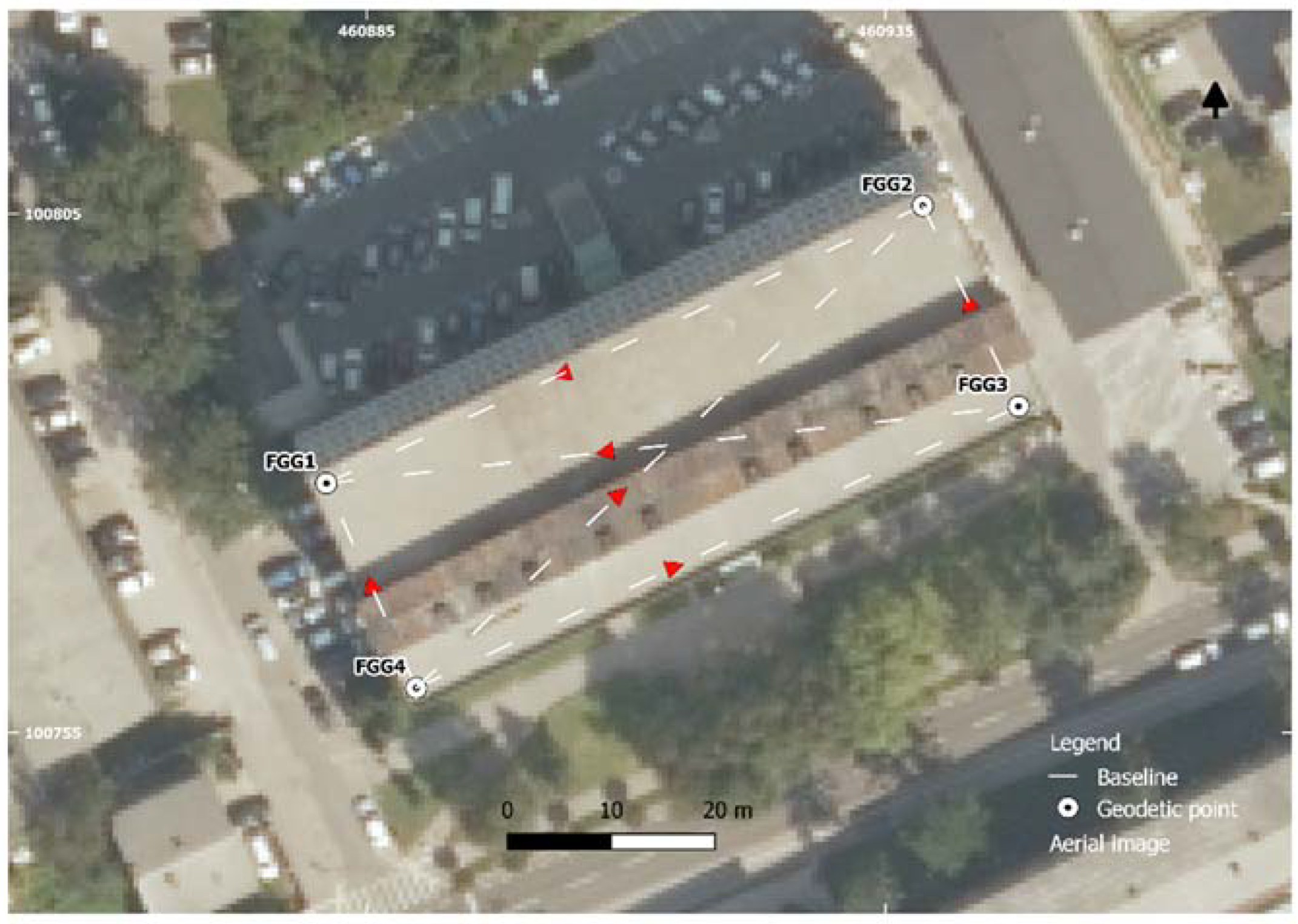
31]. The established geodetic network (Figure 1) consisted of four points and six baseline vectors. Each baseline was observed for one hour at 1 Hz, which was found to be an appropriate interval to detect displacements [32].
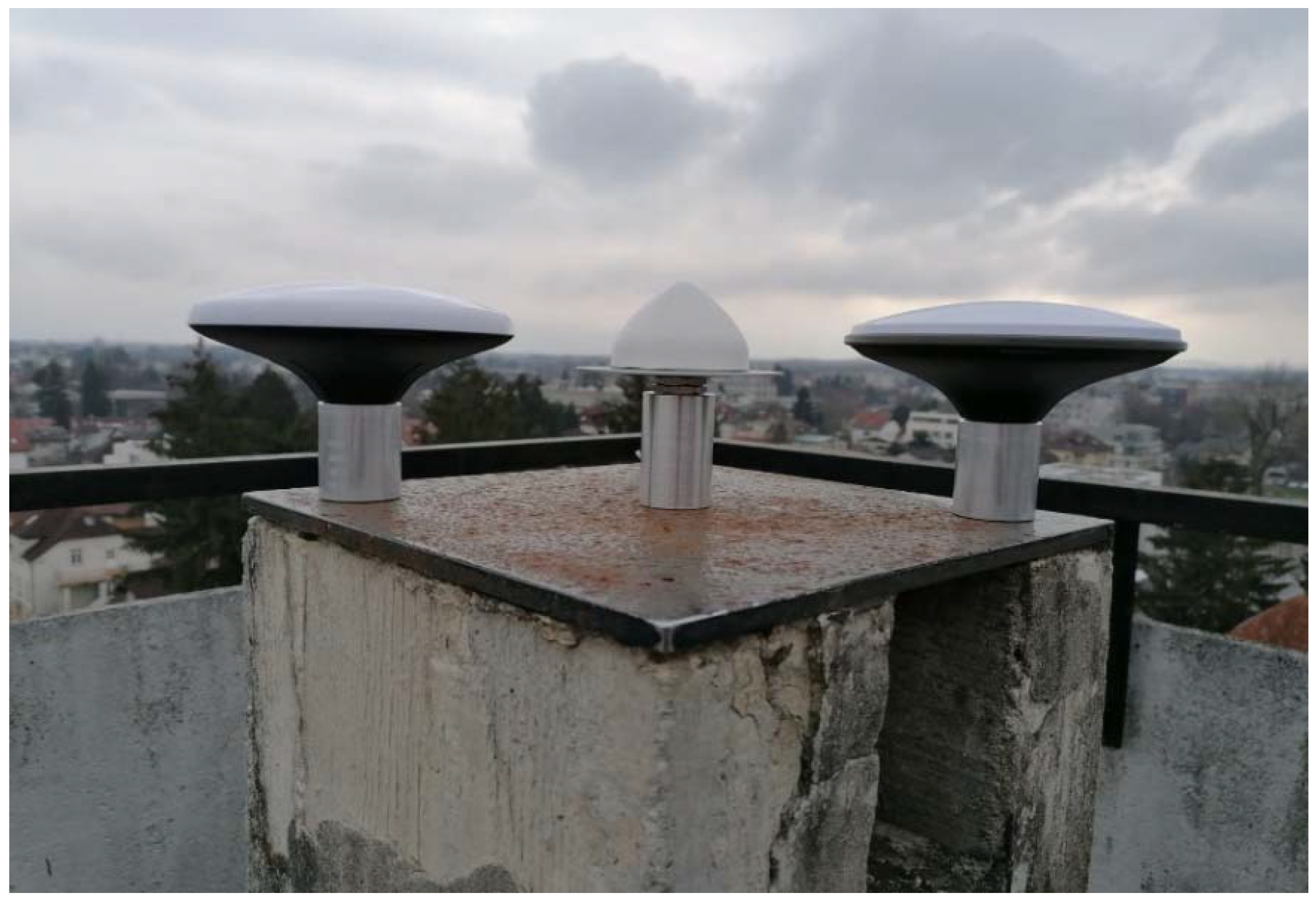
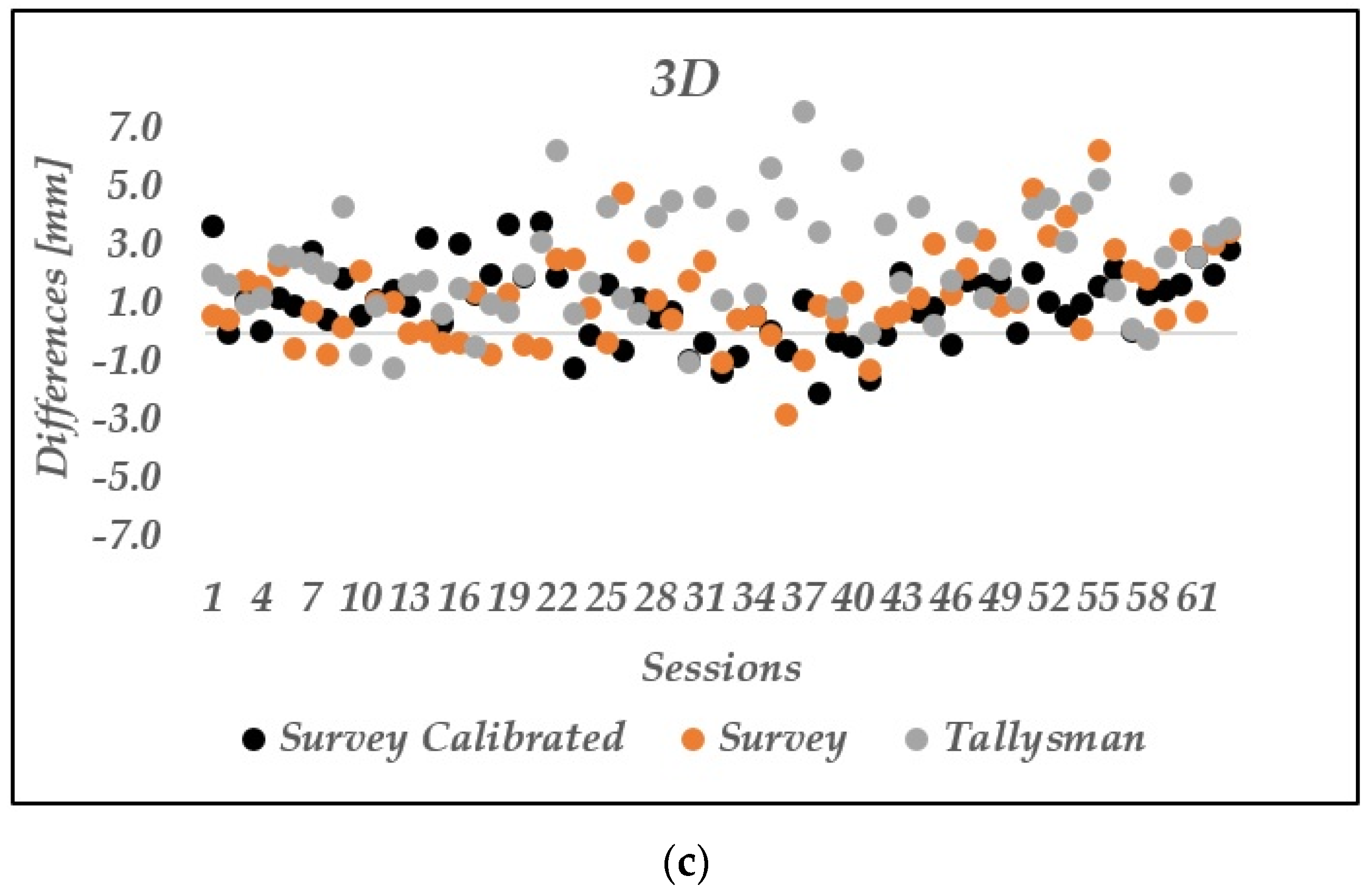
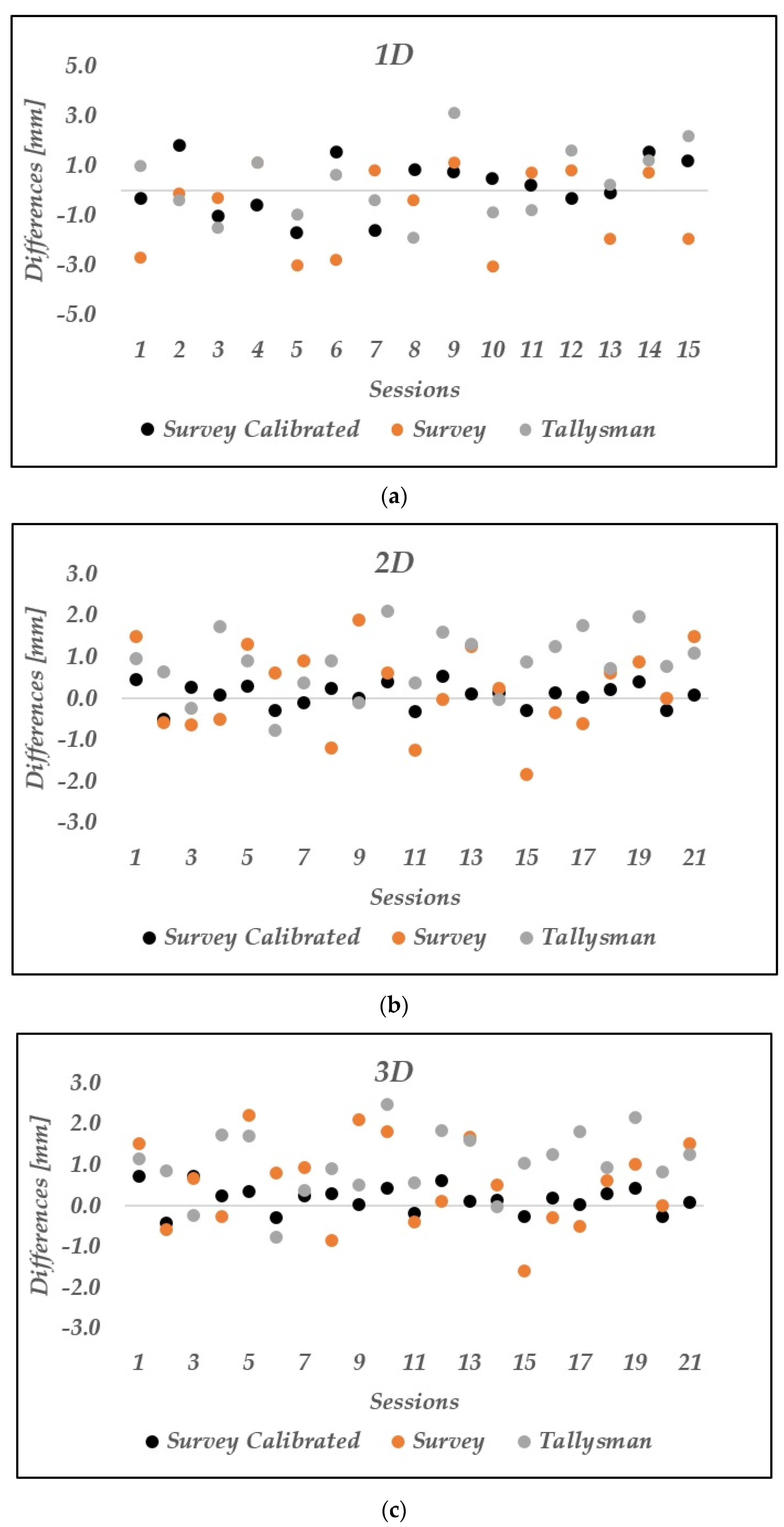
Control movements were imposed in the horizontal and vertical directions using a mechanical device and Vernier scale with high accuracy (0.05 mm) (Figure 3). The moving antenna was set on point FGG1 and was observed in the first position for one hour, after which we moved the antenna to a new position and again observed it for one hour. The procedure was repeated 7 times. The difference between consecutive positions was 2 mm, and in total, 6 movements were observed; starting from the first (session 1) to the seventh position (session 7), the rover was moved 12 mm. The same scenario was then repeated for the vertical direction, but the imposed movements between consecutive positions were 3 mm, and from the first (session 1) to the sixth position (session 6), the rover was moved 15 mm upwards. In total, six movements were imposed in the horizontal plane, and five movements were implemented in the vertical direction. The experiment was repeated for three selected low-cost antennas in the same conditions. The movements were applied to point FGG1 only, and all other points in the GNSS network remained stable. Firstly, horizontal and vertical displacements were estimated from coordinates obtained on the basis of baseline vectors only, which were estimated from points FGG4, FGG3, and FGG2 to point FGG1. Summary statistics, such as minimum, maximum, and Mean Absolute Error (MAE) of the differences between estimated and true displacements were obtained to show the differences from true movements.
Computed baseline vectors were used afterward to define a geodetic network (Figure 1). The geodetic network adjustment was carried out for each session to estimate displacements more accurately. In total, the geodetic network was adjusted 39 times, among which 18 adjustments were for vertical and 21 were for horizontal displacements. The points FGG2, FGG3, and FGG4 were used as datum points since we know a priori that they are stable. In the network adjustment, the following conditions were fulfilled [33]:
v i T P i v i = m i n ,
x i T x i = m i n   and   x ^ i = x 0 i + x i
where v i is the residual vector for the i-th session, P i is the weight matrix for the i-th session, x 0 i is the vector of approximate coordinates for the i-th session, x i is the parameter correction vector for the i-th session, and x ^ i is the vector of adjusted coordinates for the i-th session.
The data screening method (τ-test) with a significance level of 5% was used afterward for outlier detection. To analyze whether statistical equality of network precision was achieved between the corresponding sessions, the following hypothesis was established:
H 0 = E ( σ ^ i 2 ) = E ( σ ^ j 2 )
H a = E ( σ ^ i 2 ) E ( σ ^ j 2 )
where σ ^ i 2 is a posteriori variance from the i-th session, and σ ^ j 2 is a posteriori variance from the j-th session.
To determine whether the null hypothesis could be rejected, the F test was performed, defined as follows [34]:
F = σ ^ i 2 σ ^ j 2 F 1 α , f 1 , f 2
f 1 = n 1 u 1 + d
f 2 = n 2 u 2 + d
where fi is degrees of freedom for a certain session, ni is the number of observations for a certain session, ui is the number of unknowns for a certain session, d is the geodetic network datum defect, and α is the significance level.
To determine the size of the detected 1D, 2D, and 3D displacements, statistical tests were used to test the hypothesis [33,34,35,36]. Displacements were analyzed by defining the following hypothesis:
H0. 
d = 0 ; Point did not move between two sessions;
HA. 
d 0 ; Point moved between two sessions.
To determine whether the null hypothesis could be rejected, the following statistical test was performed [35]:
T = d σ d
The estimated value of the statistical test (T) was compared with its corresponding critical value from the normal (N, in the case of 1D displacements) and chi-squared ( χ 2 , in the case of 2D and 3D displacements) distributions. The critical values are defined based on the displacement dimension: the critical values are 1.96, 2.45, and 2.80 for 1D, 2D, and 3D displacements, respectively, for a significance level of 5% (α = 0.05).
The imposed 1D, 2D, and 3D movements were estimated as follows:
d 1 D = h i h j
d 2 D = ( e i e j ) 2 + ( n i n j ) 2
d 3 D = ( e i e j ) 2 + ( n i n j ) 2 + ( h i h j ) 2
where e i , n i , h i are FGG1 coordinates from the i-th session in the topocentric coordinate system, and e j , n j , h j are FGG1 coordinates from the j-th session in the topocentric coordinate system.
The network adjustment was performed in a global coordinate system, and the variance-covariance matrix for the point FGG1 was transformed to its topocentric coordinate system as follows [37]:
Σ T i = R Σ G i R T
R = [ s i n λ i c o s λ i 0 s i n φ i c o s λ i s i n φ i s i n λ i c o s φ i c o s φ i c o s λ i c o s φ i s i n λ i s i n φ i ]
where Σ G i is the variance-covariance matrix in the global coordinate system in the i-th session, R is the rotation matrix, φ i is the latitude of the point in the i-th session, and λ i is the longitude of the point in the i-th session.
The displacement precision σ d was estimated considering the error propagation law as follows [38]:
σ d 2 = J d Σ T i j J d T  
Based on the error propagation law, Jacobi matrices were defined for 1D, 2D, and 3D displacements; more details can be found in [36].
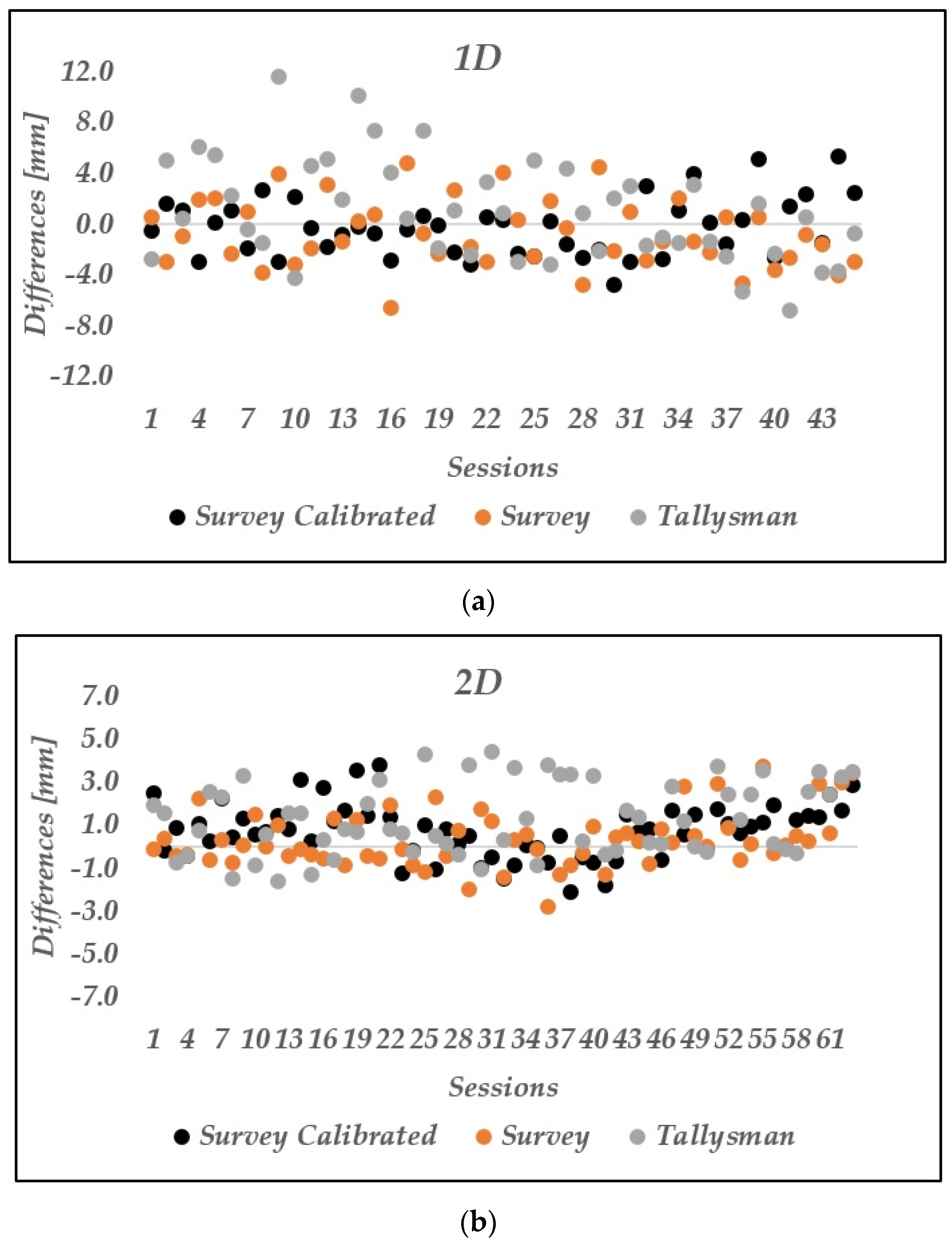
The mechanical devices could not impose spatial movements, but in order to analyze spatial displacements, the imposed horizontal movements were estimated in 3D. Movements were imposed with high accuracy (0.05 mm), and their true values are known. The MAE with respect to their true values was estimated for all displacements. Therefore, the displacement accuracy was estimated, and the difference in displacement accuracy was mainly attributed to the antenna since the other conditions (location, duration of observation, receiver type, observations) were almost the same.

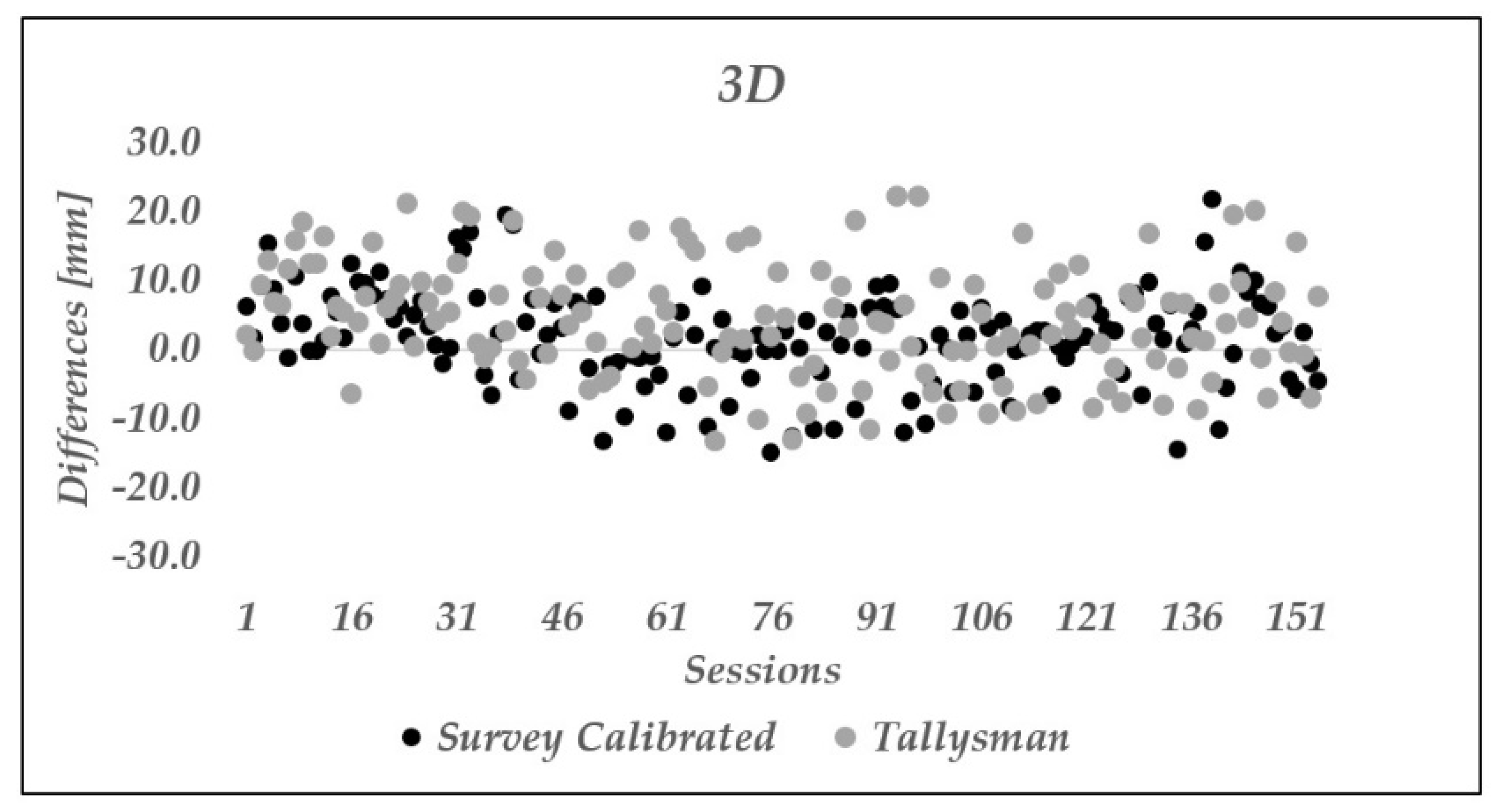
2.4. Displacement Analysis: Absolute Positioning

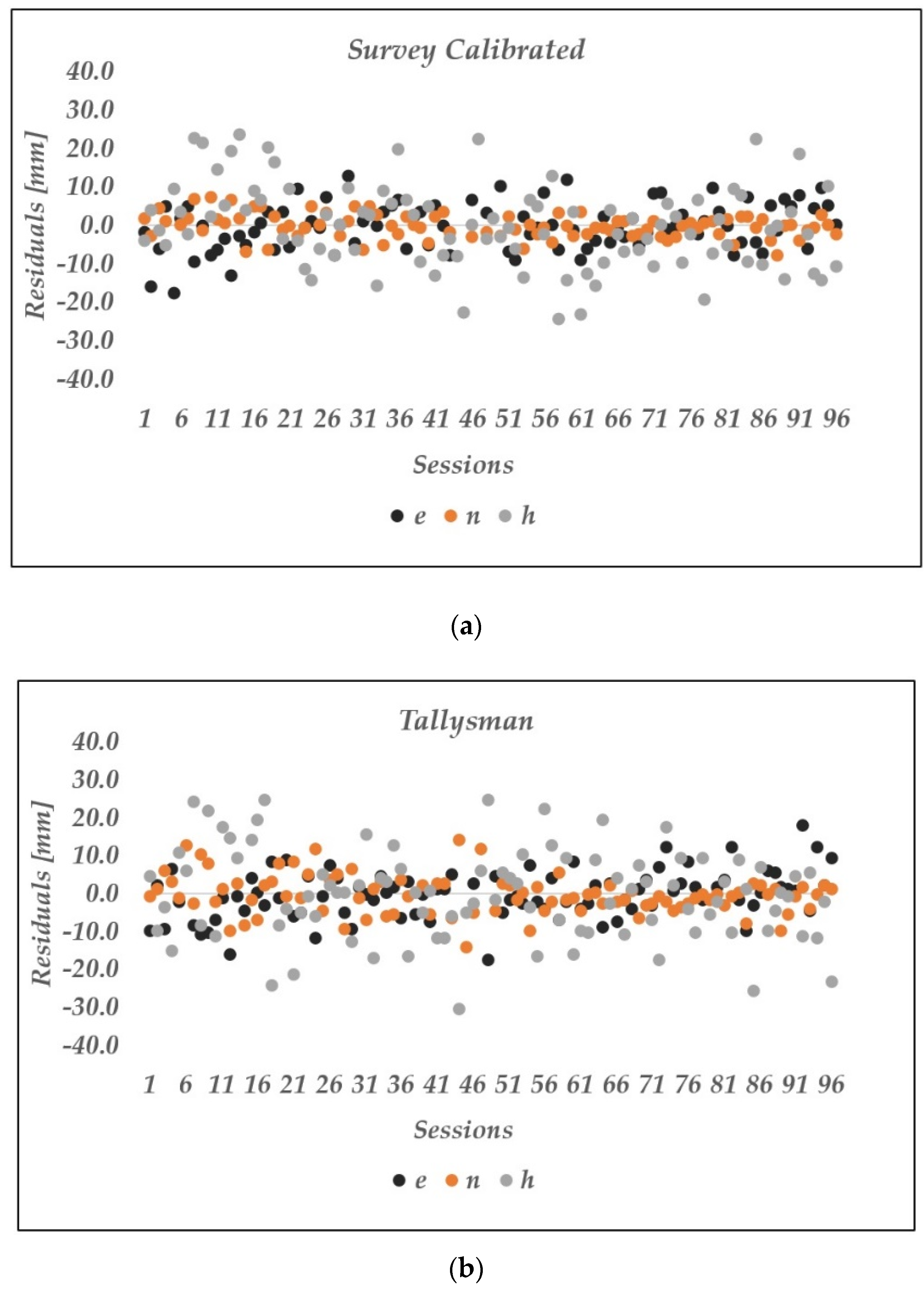
To evaluate low-cost devices in PPP mode, Survey Calibrated and Tallysman antennas were placed near point FGG1, and static observations were acquired from 1 February to 29 March 2021. In this static test, the antennas did not move. The acquired data were used to define 96 sessions, each of which contained observations for 8 h at 0.25 Hz. Then, a dynamic test was carried out in which the same mechanism was used to impose horizontal movements in steps of 10 mm. In total, seven positions were observed for 24 h, and displacements in the range of 10–60 mm were defined. As in the static test, the duration of the session was 8 h. The IGS-MGEX products, precise ephemeris (15 min, “sp3” format), and clock correction (30 s, “clk” format) were used. The satellite and receiver phase center variations were determined by using the “igs.atx” file from IGS. The Iono-Free LC and Estimated ZTD were used to eliminate the ionospheric error and the tropospheric delay, respectively. The elevation mask was set to 15°, and the DCB products from the Center of Orbit Determination in Europe were also considered.
For each session in the static test, east (e), north (n), and ellipsoid height coordinates (h) were estimated. The 3σ method was used to detect outliers, and then the RMSE, minimum, and maximum values of coordinate residuals were estimated. In monitoring applications, the movements can be in any direction; thus, we estimated them in the 3D coordinate system. The statistical hypotheses for spatial movements defined in the previous subsection were used to identify the range of detected displacements.

2.5. Low-Cost and Geodetic GNSS Instruments: A Comparison in Terms of Observations

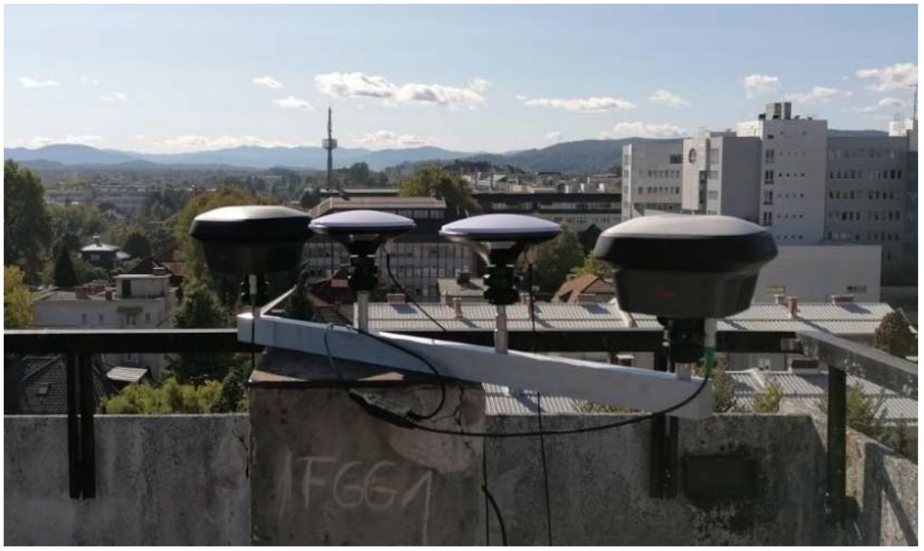
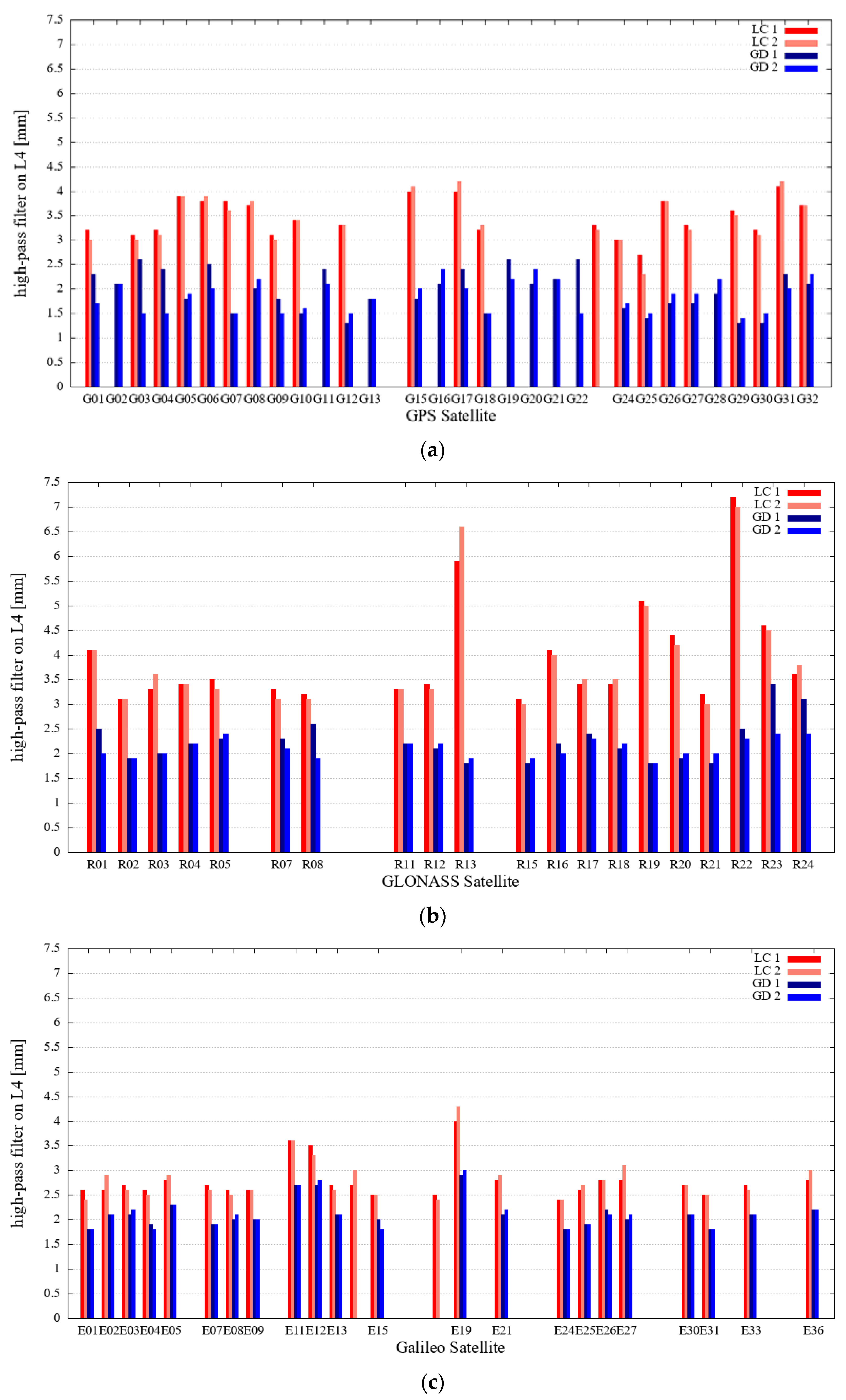
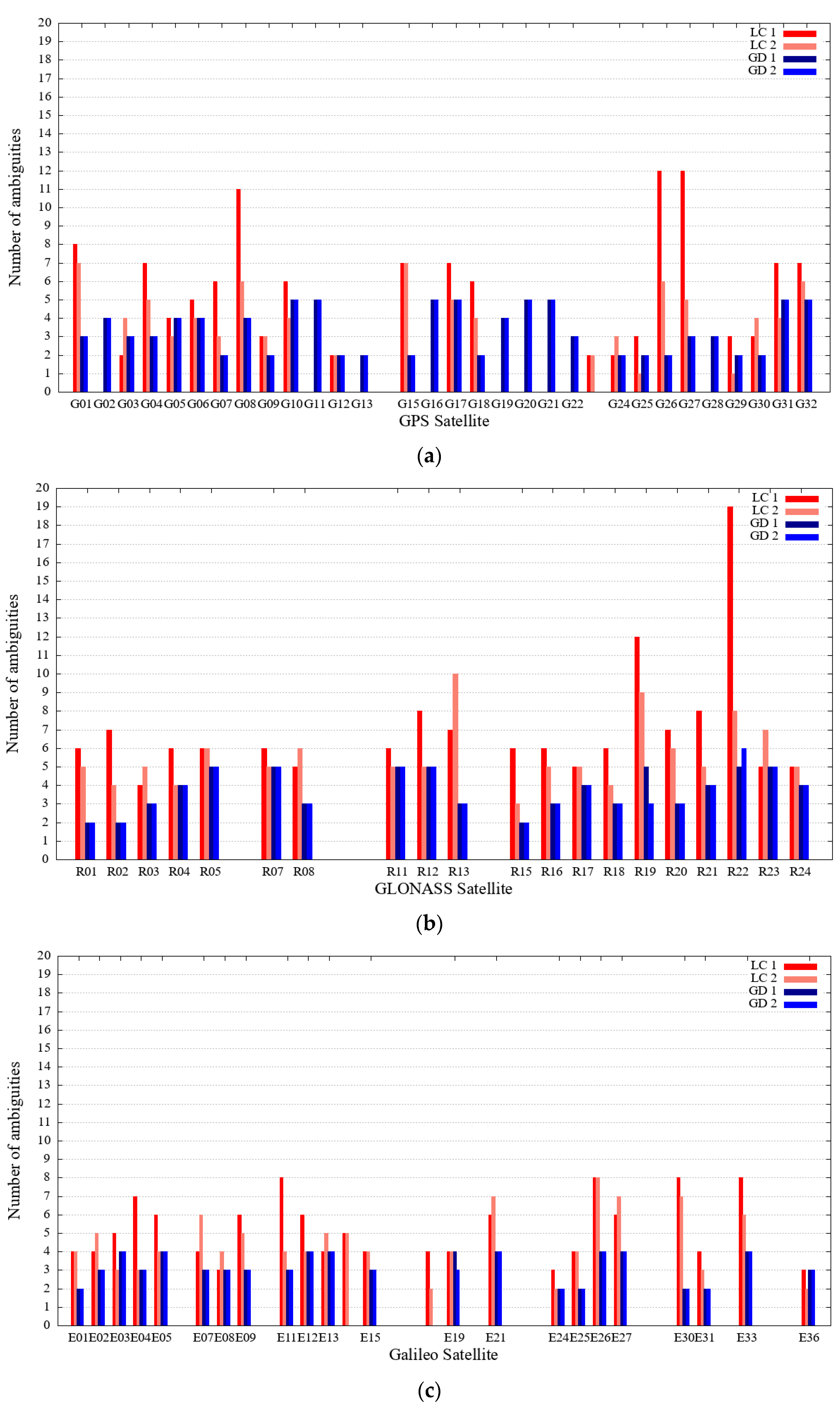
To use low-cost GNSS instruments for displacement detection purposes, they must be able to perform with a similar level of quality and reliability to geodetic GNSS instruments. In the test described in this sub-section, comparisons were made between two low-cost (simpleRTK2B V1 receiver and Survey Calibrated antenna) and two geodetic (Leica GS18 receiver and LEIGS18 antenna) GNSS instruments. Data used for comparison comprise almost 48 h of static observations that were acquired at 1 Hz (Figure 4).
The performance of all instruments used was analyzed with the help of several linear combinations of raw GNSS observations, where the geometry-free linear combination (L4) is of particular interest. All of the previously mentioned linear combinations can also be used for cycle slip detection and repair [39,40,41]. One of the parameters that indicate the reliability of the GNSS instrument is the number of cycle slips (i.e., ambiguities) that occur during the survey, where the lowest possible number of cycle slips is desirable.
The most important quantity for precise position determination in the case of GNSS is the quality of phase observations with both carriers. The noise of phase observations can be determined with the geometry-free linear combination L4. However, since L4 slowly changes over time due to temporal changes in ionospheric bias, this linear combination must be filtered to remove the low-frequency trend [41]. For each satellite tracked by four GNSS devices, the L4 linear combination was filtered with a simple 3-point high-pass filter as follows:
H P = L 4 i 1 2   L 4 i + L 4 i + 1
where i represents the index of an epoch. The variable H P contains only amplified (by 6 ) noise of linear combination L4.

3. Results

Displacements were first estimated only from baseline vectors and then from the coordinates obtained after geodetic adjustment of the network. The differences from the true values of the estimated 1D, 2D, and 3D displacements on the basis of only baseline vectors are shown in Figure 5. Table 4 presents the summary statistics for the obtained differences, such as MAE, the minimum, and the maximum values of differences, for all low-cost GNSS antennas used.
The geodetic adjustment was carried out for each of the selected antennas separately, and the a posteriori standard deviation was estimated for sessions in which vertical (Table 5) and horizontal movements (Table 6) were imposed.
Coordinates obtained from the geodetic adjustment were used to calculate displacements, and the presented statistical tests were applied to identify the sizes of detected movements for the selected antennas. Vertical movements were imposed in steps of 3 mm, while horizontal movements were imposed in steps of 2 mm and were also estimated in a 3D coordinate system. The results from the detection of 1D (vertical), 2D (horizontal), and 3D (spatial) displacements are shown in Table 7, Table 8 and Table 9, respectively.
For the estimated movements, the MAE was obtained to present the accuracy of 1D, 2D, and 3D displacements for each of the used antennas. These results are presented in Table 10 and show that the Survey Calibrated antenna outperforms the others. The differences in the displacements from the true values are also shown graphically in Figure 6.
Low-cost devices were evaluated in PPP mode. The residuals of the obtained coordinates are presented in Figure 7, while the related statistics are reported in Table 11. In a dynamic test, movements of known size were imposed, and statistical tests were used to analyze the range of detected movements in PPP (Table 12). The MAE values of differences from true values are presented in Table 13 and are also graphically shown in Figure 8.
Observations obtained using low-cost devices were additionally compared with those obtained with high-end geodetic GNSS instruments. The final number of determined phase ambiguities (after cycle slip detection and repair) is shown for all satellites in Figure 9, where the top graph represents the number of ambiguities for GPS satellites, the middle presents the values for GLONASS satellites, and the bottom shows the results for Galileo satellites. Both geodetic GNSS instruments (denoted as GD 1 and GD 2) are represented with blue bars, whereas the low-cost GNSS instruments (denoted as LC 1 and LC 2) are indicated by red bars. The Root-Mean-Squared (RMS) values of variable HP (high-pass-filtered L4 linear combination) were estimated for each satellite and are shown in Figure 10. Geodetic (GD1 and GD2) and low-cost (LC 1 and LC 2) instruments are denoted in Figure 10 as in Figure 9.

4. Discussions

Imposed 1D, 2D, and 3D movements were estimated from baseline vectors only to show the differences from the true movements in a case where adjustment of the geodetic network is not carried out (Figure 5). The MAE of 2D displacements is in the range of 1.0–1.7 mm; for 3D displacements, the MAE is in the range of 1.3–2.5 mm, while the value of MAE is greater for 1D displacements, ranging from 1.9 to 3.3 mm (Table 4). However, the differences between MAE of used antennas are at the millimeter level or even smaller.
To increase the accuracy of estimated displacements, the geodetic adjustment of the network was carried out, where the data were defined by three points of the geodetic network that did not have movements between sessions. The a posteriori standard deviations were estimated (Table 5 and Table 6) for sessions when vertical and horizontal movements were imposed. With a significance level of 5%, we could not reject the null hypothesis, and homogenous network precision was obtained in all combinations between sessions. The a posteriori standard deviation is in the range of 0.9–2.3 mm for all sessions. The results from Table 5 and Table 6 show that using the Survey Calibrated antenna, where antenna calibration parameters are known, results in higher precision of estimated positions. The improvement may be as much as 50%. However, the differences are in the order of millimeters or even smaller.
Vertical movements were imposed in steps of 3 mm and ranged from 3 to 15 mm, and horizontal movements were in steps of 2 mm and ranged from 2 to 12 mm. For 1D displacement detection, we were not able to detect 3 mm with statistical significance (more than 95%) with any of the used antennas in combination with the ZED-F9P GNSS chip (Table 7). Displacements were detected in 60%, 20%, and 20% of cases for Survey Calibrated, Survey, and Tallysman antenna, respectively. The Survey Calibrated antenna can detect 6 mm displacements; however, this does not hold true for Survey and Tallysman antennas (only 75%). Displacements with a size of 9 mm were detected (100%) with all three GNSS antennas.
Horizontal displacements were imposed in steps of 2 mm. Based on the results presented in Table 8, it can be concluded that 2 mm displacements cannot be detected by low-cost GNSS instruments. The Survey Calibrated and the Tallysman antennas were able to detect 4 mm displacements, while the Survey antenna did not. Horizontal displacements of 6 mm or larger could be detected (100%) by the three used GNSS devices.
In monitoring natural objects and man-made structures, movements can occur in any direction (spatially), so we estimated the imposed horizontal movements in a 3D coordinate system. From the results presented in Table 9, we can conclude that 6 mm displacements can be detected by all antennas, while a low percentage (60%) of 4 mm displacements were detected with the Survey antenna. The smallest imposed movements (2 mm) were not detected by low-cost GNSS instruments. Only 17% of considered displacements of the magnitude 2 mm were detected. The results presented in Table 7, Table 8 and Table 9 indicate that the Survey Calibrated antenna had better positioning performance. The Survey Calibrated antenna outperformed the others in terms of the sizes of detected 1D, 2D, and 3D movements. The Tallysman antenna was better than the Survey antenna in detecting 2D and 3D movements, while they provided the same results when detecting 1D movements. Neither antenna performed as well as the Survey Calibrated antenna.
Horizontal and vertical movements were imposed by a special mechanism with high accuracy. Therefore, the true values of displacements are well known. The MAE values with respect to the true values were estimated for all displacements (Table 10).
The Survey Calibrated antenna has a smaller MAE (0.9 mm) of 1D displacements than both uncalibrated antennas. For the Survey and Tallysman antennas, the MAE values are 1.2 mm, and 1.3 mm, respectively. The results from Table 10 for 2D displacements also highlight the superior performance of the Survey Calibrated antenna, as its MAE is 0.2 mm, while the MAE values are 0.9 mm and 1.0 mm for the Survey and Tallysman antennas, respectively. For 3D displacements, the MAE values of Survey and Tallysman are 1.0 mm and 1.1 mm, while for Survey Calibrated, the value is smaller (0.3 mm). It can be emphasized here that the MAE of 2D displacements is smaller than that of 3D in all cases, while for 1D, the value of MAE is greater since the number of imposed movements (sample size) differed between the two tests. The Survey Calibrated antenna has known calibration parameters even though it is a low-cost antenna. Based on the results presented in Table 10, Survey Calibrated had higher displacement accuracy in all cases, and its performance was better than the two uncalibrated antennas: The displacement accuracy was almost the same between them but lower than that of Survey Calibrated. Differences between true and estimated 1D, 2D, and 3D movements are shown graphically in Figure 5. The variations are again in favor of Survey Calibrated for 1D, 2D, and 3D displacements. Variations are larger for 1D differences, while the 2D and 3D differences have almost the same variations. The differences from the true values of displacements obtained with geodetic network adjustment (Figure 6) are smaller compared with those estimated from baseline vectors only (Figure 5).
In the static test (PPP), low-cost devices showed satisfactory performance. The RMSE for horizontal components is at the sub-centimeter-level for east (6.1 mm) and north (3.1 mm) components for the Survey Calibrated antenna. The ellipsoid height estimated with GNSS observations has lower precision compared with the horizontal components, and the uncertainty of the ellipsoid height for Survey Calibrated is 10.8 mm (Table 11). For the Tallysman antenna, the values of RMSE are 6.3 mm, 5.1 mm, and 11.7 mm for the east, north, and ellipsoid height, respectively (Table 11). Spatial displacements of 20 mm were detected by both antennas: The Tallysman antenna detected 88.9% of imposed movements, while Survey Calibrated detected 91.7% (Table 12). Displacements greater than 20 mm were detected by both antennas in all cases. The MAE is 5.4 mm for Survey Calibrated and is greater (7.4 mm) for Tallysman (Table 13).
The comparison of low-cost and geodetic instruments showed better performance for the latter. In all cases (all satellites from all systems), the number of cycle slips is higher for the low-cost instruments compared with the geodetic ones, but the increase is not significant (Figure 9). After all, there are still enough continuous GNSS data for each ambiguity to be estimated with sufficient quality. The represented RMS values in the graphs in Figure 10 show slightly higher values of phase noise for low-cost GNSS instruments (red bars) compared with the noise of phase observations obtained with geodetic GNSS instruments (blue bars). However, the noise level of low-cost GNSS instruments is still at the millimeter level, which assures a millimeter level of derived results, i.e., adjusted coordinates or baseline components.

5. Conclusions

Low-cost GNSS receivers have been tested in different applications for positioning and navigation purposes. Taking into account their cost and the demonstrated performance, these GNSS devices can be suitable sensors for geodetic monitoring in areas with a high risk of instrument damage. Recently, multi-frequency GNSS receivers and calibrated low-cost antennas have become available on the market, which makes them more comparable to high-end geodetic GNSS instruments.
In this study, the u-blox ZED-F9P multi-frequency receiver in combination with Survey Calibrated, Survey, and Tallysman antennas was tested for displacement detection. The main objectives were to identify the range of displacements detected by low-cost devices in relative and absolute positioning modes and analyze the differences between these low-cost antennas. The results from this study lead to the following conclusions:
  • The low-cost Survey Calibrated antenna performed better in relative positioning than the non-calibrated antennas Survey and Tallysman. The smallest MAE for 1D, 2D, and 3D displacements estimated after the geodetic adjustment was obtained by the Survey Calibrated antenna, which also had the best performance in terms of the magnitude of detected displacements.
  • For 1D displacement detection, Survey and Tallysman antennas had similar performance. The MAE for 1D was almost equal between the two, and the size of detected displacements was 9 mm. The Survey Calibrated antenna had a slightly smaller MAE, and the size of detected displacements was 6 mm.
  • The Tallysman antenna and Survey Calibrated antenna detected 2D displacements of 4 mm, which was not the case for the Survey antenna. The size of displacements that were detected at a high percentage by the Survey antenna was 6 mm.
  • For spatial displacement (3D) detection, the size of detected displacements was the same for all antennas as for 2D displacements. Displacements of 4 mm were detected by Survey Calibrated and Tallysman, while for the Survey antenna, the size of detected displacements was 6 mm.
  • Displacements of 20 mm or greater were detected by low-cost GNSS devices in absolute positioning mode. The performance of Survey Calibrated was also slightly better than that of Tallysman in PPP.
  • All three antennas were able to detect spatial displacements smaller than 10 mm in relative positioning mode and can be used to monitor many engineering buildings. In absolute positioning mode, displacements of 20 mm were detected, which is adequate for monitoring natural objects (landslides).
  • Geodetic GNSS instruments had better performance than low-cost instruments. The number of cycle slips and the noise of phase observations were best with geodetic GNSS instruments. However, the difference in cycle slips among them was not very large, and the noise of phase observations was at a level of a few millimeters for low-cost devices.
All tests were carried out in an open-sky area and over short baselines to evaluate the antenna’s impact on positioning performance and compare low-cost uncalibrated and calibrated antennas. The presented results from this study should be treated as preliminary. To better evaluate low-cost GNSS instruments, more tests will be carried out over medium and long baselines, and geodetic and low-cost GNSS instruments and different combinations thereof will be used. For a more in-depth analysis of the potential of these sensors for geodetic monitoring purposes, we will attempt to test them in harsh environments, and a more detailed analysis will be carried out, in terms of observations. A real natural object (landslide) or man-made object will be monitored, and other geodetic instrumentations may be used to evaluate the performance of low-cost GNSS devices.

Author Contributions

Conceptualization, V.H. and B.S.; methodology, V.H., B.S. and T.A.; software, V.H.; formal analysis, V.H.; investigation, V.H.; data curation, V.H.; writing—original draft preparation, V.H.; writing—review and editing, V.H., B.S., T.A. and O.S.; visualization, V.H.; supervision, O.S. and B.S. All authors have read and agreed to the published version of the manuscript.

Funding

The authors acknowledge the financial support from the Slovenian Research Agency-ARRS (research core funding No. P2-0227 Geoinformation infrastructure and sustainable spatial development of Slovenia).

Data Availability Statement

Publicly available datasets were analyzed in this study. This data can be founded here: https://unilj-my.sharepoint.com/:f:/g/personal/vhamza_fgg_uni-lj_si/EltFQraUd5lKjY7S-bjvJb8BLYbQfGUC0U63Yrmb4ZL0cg?e=si4YIQ (accessed on 24 June 2021).

Acknowledgments

This study is a part of the Ph.D. research of the corresponding author. We are grateful to anonymous reviewers and editors for their suggestions.

Conflicts of Interest

The authors declare no conflict of interest.

References

  1. Xiao, R.; Shi, H.; He, X.; Li, Z.; Jia, D.; Yang, Z. Deformation Monitoring of Reservoir Dams Using GNSS: An Application to South-to-North Water Diversion Project, China. IEEE Access 2019, 7, 54981–54992. [Google Scholar] [CrossRef]
  2. Barzaghi, R.; Cazzaniga, N.; De Gaetani, C.; Pinto, L.; Tornatore, V. Estimating and Comparing Dam Deformation Using Classical and GNSS Techniques. Sensors 2018, 18, 756. [Google Scholar] [CrossRef] [Green Version]
  3. Yi, T.-H.; Li, H.-N.; Gu, M. Experimental Assessment of High-Rate GPS Receivers for Deformation Monitoring of Bridge. Measurement 2013, 46, 420–432. [Google Scholar] [CrossRef]
  4. Yu, J.; Yan, B.; Meng, X.; Shao, X.; Ye, H. Measurement of Bridge Dynamic Responses Using Network-Based Real-Time Kinematic GNSS Technique. J. Surv. Eng. 2016, 142, 04015013. [Google Scholar] [CrossRef]
  5. Kaloop, M.; Elbeltagi, E.; Hu, J.; Elrefai, A. Recent Advances of Structures Monitoring and Evaluation Using GPS-Time Series Monitoring Systems: A Review. IJGI 2017, 6, 382. [Google Scholar] [CrossRef] [Green Version]
  6. Im, S.B.; Hurlebaus, S.; Kang, Y.J. Summary Review of GPS Technology for Structural Health Monitoring. J. Struct. Eng. 2013, 139, 1653–1664. [Google Scholar] [CrossRef]
  7. Biagi, L.; Grec, F.; Negretti, M. Low-Cost GNSS Receivers for Local Monitoring: Experimental Simulation, and Analysis of Displacements. Sensors 2016, 16, 2140. [Google Scholar] [CrossRef] [PubMed] [Green Version]
  8. Caldera, S.; Realini, E.; Barzaghi, R.; Reguzzoni, M.; Sansò, F. Experimental Study on Low-Cost Satellite-Based Geodetic Monitoring over Short Baselines. J. Surv. Eng. 2016, 142, 04015016. [Google Scholar] [CrossRef]
  9. Garrido-Carretero, M.S.; de Lacy-Pérez de los Cobos, M.C.; Borque-Arancón, M.J.; Ruiz-Armenteros, A.M.; Moreno-Guerrero, R.; Gil-Cruz, A.J. Low-Cost GNSS Receiver in RTK Positioning under the Standard ISO-17123-8: A Feasible Option in Geomatics. Measurement 2019, 137, 168–178. [Google Scholar] [CrossRef]
  10. Cina, A.; Piras, M. Performance of Low-Cost GNSS Receiver for Landslides Monitoring: Test and Results. Geomat. Nat. Hazards Risk 2015, 6, 497–514. [Google Scholar] [CrossRef]
  11. Odolinski, R.; Teunissen, P.J.G. Single-Frequency, Dual-GNSS versus Dual-Frequency, Single-GNSS: A Low-Cost and High-Grade Receivers GPS-BDS RTK Analysis. J. Geod. 2016, 90, 1255–1278. [Google Scholar] [CrossRef]
  12. Tsakiri, M.; Sioulis, A.; Piniotis, G. Compliance of Low-Cost, Single-Frequency GNSS Receivers to Standards Consistent with ISO for Control Surveying. Int. J. Metrol. Qual. Eng. 2017, 8, 11. [Google Scholar] [CrossRef] [Green Version]
  13. Poluzzi, L.; Tavasci, L.; Corsini, F.; Barbarella, M.; Gandolfi, S. Low-Cost GNSS Sensors for Monitoring Applications. Appl. Geomat. 2020, 12, 35–44. [Google Scholar] [CrossRef]
  14. Barzaghi, R.; Reguzzoni, M.; De Gaetani, C.I.; Caldera, S.; Rossi, L. Cultural Heritage Monitoring by Low-Cost GNSS Receivers: A Feasibility Study for San Guadenzio’s Cupola, Novara. Int. Arch. Photogramm. Remote Sens. Spat. Inf. Sci. 2019, XLII-2/W11, 209–216. [Google Scholar] [CrossRef] [Green Version]
  15. Wielgocka, N.; Hadas, T.; Kaczmarek, A.; Marut, G. Feasibility of Using Low-Cost Dual-Frequency GNSS Receivers for Land Surveying. Sensors 2021, 21, 1956. [Google Scholar] [CrossRef]
  16. Jackson, J.; Davis, B.; Gebre-Egziabher, D. A Performance Assessment of Low-Cost RTK GNSS Receivers. In Proceedings of the 2018 IEEE/ION Position, Location and Navigation Symposium (PLANS), Monterey, CA, USA, 23–26 April 2018; pp. 642–649. [Google Scholar]
  17. Guo, L.; Jin, C.; Liu, G. Evaluation on Measurement Performance of Low-Cost GNSS Receivers. In Proceedings of the 2017 3rd IEEE International Conference on Computer and Communications (ICCC), Chengdu, China, 13–16 December 2017. [Google Scholar]
  18. Bellone, T.; Dabove, P.; Manzino, A.M.; Taglioretti, C. Real-Time Monitoring for Fast Deformations Using GNSS Low-Cost Receivers. Geomat. Nat. Hazards Risk 2016, 7, 458–470. [Google Scholar] [CrossRef] [Green Version]
  19. Odolinski, R.; Teunissen, P.J.G. Low-Cost, High-Precision, Single-Frequency GPS–BDS RTK Positioning. GPS Solut. 2017, 21, 1315–1330. [Google Scholar] [CrossRef]
  20. Odolinski, R.; Teunissen, P.J.G. Low-Cost, 4-System, Precise GNSS Positioning: A GPS, Galileo, BDS and QZSS Ionosphere-Weighted RTK Analysis. Meas. Sci. Technol. 2017, 28, 125801. [Google Scholar] [CrossRef] [Green Version]
  21. Odolinski, R.; Teunissen, P.J.G. Best Integer Equivariant Estimation: Performance Analysis Using Real Data Collected by Low-Cost, Single- and Dual-Frequency, Multi-GNSS Receivers for Short-to Long-Baseline RTK Positioning. J. Geod. 2020, 94, 91. [Google Scholar] [CrossRef]
  22. Mahato, S.; Shaw, G.; Santra, A.; Dan, S.; Kundu, S.; Bose, A. Low Cost GNSS Receiver RTK Performance in Forest Environment. In Proceedings of the 2020 URSI Regional Conference on Radio Science (URSI-RCRS), Varanasi, India, 12–14 February 2020; pp. 1–4. [Google Scholar]
  23. Semler, Q.; Mangin, L.; Moussaoui, A.; Semin, E. Development of a Low-Cost Centimetric GNSS Solution for Android Apllications. In Proceedings of the ISPRS-International Archives of the Photogrammetry, Remote Sensing and Spatial Information Sciences, Strasbourg, France, 2 December 2019; Volume XLII-2/W17, pp. 309–314. [Google Scholar]
  24. Krietemeyer, A.; van der Marel, H.; van de Giesen, N.; ten Veldhuis, M.-C. High Quality Zenith Tropospheric Delay Estimation Using a Low-Cost Dual-Frequency Receiver and Relative Antenna Calibration. Remote Sens. 2020, 12, 1393. [Google Scholar] [CrossRef]
  25. Notti, D.; Cina, A.; Manzino, A.; Colombo, A.; Bendea, I.H.; Mollo, P.; Giordan, D. Low-Cost GNSS Solution for Continuous Monitoring of Slope Instabilities Applied to Madonna Del Sasso Sanctuary (NW Italy). Sensors 2020, 20, 289. [Google Scholar] [CrossRef] [PubMed] [Green Version]
  26. Šegina, E.; Peternel, T.; Urbančič, T.; Realini, E.; Zupan, M.; Jež, J.; Caldera, S.; Gatti, A.; Tagliaferro, G.; Consoli, A.; et al. Monitoring Surface Displacement of a Deep-Seated Landslide by a Low-Cost and near Real-Time GNSS System. Remote Sens. 2020, 12, 3375. [Google Scholar] [CrossRef]
  27. U-blox ZED-F9P. Available online: https://www.u-blox.com/sites/default/files/ZED-F9P_DataSheet_%28UBX-17051259%29.pdf (accessed on 13 February 2020).
  28. NGS Survey Calibrated GNSS Multiband Antenna. Available online: https://www.ngs.noaa.gov/ANTCAL/index.xhtml# (accessed on 14 October 2020).
  29. Ardusimple GNSS Antennas. Available online: https://www.ardusimple.com/ (accessed on 14 October 2020).
  30. Tallysman Tallysman TW3882. Available online: https://www.tallysman.com/ (accessed on 14 October 2020).
  31. Everett, T. RTKLIB Demo5_b33b. Available online: https://rtkexplorer.com/downloads/rtklib-code/ (accessed on 4 January 2020).
  32. Semler, J.; Heunecke, O.; Pink, S.; Schuhbäck, S. Developments towards a Low-Cost GNSS Based Sensor Network for the Monitoring of Landslides. In Proceedings of the 13th FIG International Symposium on Deformation Measurements and Analysis, Lisbon, Portugal, 12–15 May 2008. [Google Scholar]
  33. Kuang, S. Geodetic Network Analysis and Optimal Design: Concepts and Applications; Ann Arbor Press: Chelsea, MI, USA, 1996; ISBN 978-1-57504-044-8. [Google Scholar]
  34. Caspary, W.F.; Rüeger, J.M. Concepts of Network and Deformation Analysis; 2nd corr. imp; School of Surveying: Kensington, UK, 1988; ISBN 978-0-85839-044-7. [Google Scholar]
  35. Koch, K.-R. Parameter Estimation and Hypothesis Testing in Linear Models; Springer: Berlin, Germany; London, UK, 2011; ISBN 978-3-642-08461-4. [Google Scholar]
  36. Savšek, S. An Alternative Approach to Testing Displacements in a Geodetic Network. Geod. Vestn. 2017, 61, 387–411. [Google Scholar] [CrossRef]
  37. Soler, T.; Chin, M. On Transformation of Covariance Matrices between Local Cartesian Coordinate Systems and Commutative Diagrams. In Proceedings of the 45th Annual Meeting ASP-ACSM Convention, Washington, DC, USA, January 1985; Available online: https://www.acsm.org/annual-meeting/future-past-meetings/past-meetings (accessed on 4 January 2020).
  38. Mikhail, E.M.; Gracie, G. Analysis and Adjustment of Survey Measurements; Van Nostrand Reinhold Co: New York, NY, USA, 1981; ISBN 978-0-442-25369-1. [Google Scholar]
  39. Teunissen, P.J.G.; Montenbruck, O. (Eds.) Springer Handbook of Global Navigation Satellite Systems; Springer International Publishing: Cham, Switzerland, 2017; ISBN 978-3-319-42926-7. [Google Scholar]
  40. Leick, A.; Rapoport, L.; Tatarnikov, D. GPS Satellite Surveying, 4th ed.; Wiley: Hoboken, NJ, USA, 2015; ISBN 978-1-118-67557-1. [Google Scholar]
  41. Estey, L.H.; Meertens, C.M. TEQC: The Multi-Purpose Toolkit for GPS/GLONASS Data. GPS Solut. 1999, 3, 42–49. [Google Scholar] [CrossRef]
Figure 1. Study area: roof of UL FGG building.
Applsci 11 06666 g001
Figure 2. Low-cost GNSS antennas: Survey (left), Tallysman TW3882 (middle), and Survey Calibrated (right).
Applsci 11 06666 g002
Figure 3. Imposed controlled movements: (a) Horizontal movements; (b) vertical movements.
Applsci 11 06666 g003
Figure 4. Geodetic and low-cost GNSS devices in the four-point metal arm.
Applsci 11 06666 g004
Figure 5. Differences between estimated and true movements from baseline vectors only: (a) 1D differences, (b) 2D differences, and (c) 3D differences.
Applsci 11 06666 g005aApplsci 11 06666 g005b
Figure 6. Differences between estimated and true movements: (a) 1D differences, (b) 2D differences, and (c) 3D differences.
Applsci 11 06666 g006
Figure 7. Residuals for east (e), north (n), and ellipsoid height (h) in static test (PPP): (a) Survey Calibrated; (b) Tallysman.
Applsci 11 06666 g007
Figure 8. Differences between estimated and true 3D displacements (PPP).
Applsci 11 06666 g008
Figure 9. The number of phase ambiguities for each satellite for both low-cost instruments (red bars) as well as for both geodetic instruments (blue bars): (a) GPS, (b) GLONASS, and (c) Galileo.
Applsci 11 06666 g009
Figure 10. RMS values of the high-pass-filtered L4 linear combination for all satellite systems for both low-cost instruments (red bars) as well as for both geodetic instruments (blue bars)): (a) GPS, (b) GLONASS, and (c) Galileo.
Applsci 11 06666 g010
Table 1. Specifications for GNSS devices used.
SpecificationsSimpleRTK2B V1
GNSS chipZED-F9P
ConstellationsGPS, GLONASS, Galileo, BeiDou
FrequenciesL1/L2
SignalsL1C/A, L1OF, E1, B1l, L2C, L2OF, E5b, B2l
Channels184
Weight19.5 g
Size69 mm × 53 mm
Ports5
MessagesUBX, NMEA, RTCM3
Supply voltage range4.5–5.5 V
Supply current80 mA
Table 2. Specifications for GNSS antennas used.
AntennaSurvey CalibratedSurveyTallysman
Weight535 g535 g185 g
FrequencyL1/L2L1/L2L1/L2
Price150 EUR90 EUR300 EUR
Calibration YesNoNo
LNA Gain40 db40 db35 db
LNA Noise figure 1.5   db 1.5   db 2.5   db
Supply voltage range3–12 V DC3–5.5 V DC2.5–16 V DC
Supply current50 mA45 mA24 mA
Phase center error1 mm3 mm/
Ingress protectionIP67IP66IP67
Mounting methodScrewScrewScrew
Size151.5 mm × 61.5 mm146.5 mm × 62.5 mm66.5 mm × 48 mm
Operating temperature 40     to + 85   40     to + 85   40     to + 85  
Table 3. Parameters used in the data processing.
ParametersRTKLIB
ObservationsL1, L2
Duration1 h
ConstellationsGPS, GLONASS, Galileo
AmbiguityFix and hold (LAMBDA)
Elevation mask15°
Table 4. Statistics for 1D, 2D, and 3D displacements estimated from baseline vectors only.
AntennaSurvey CalibratedSurveyTallysman
Dimension1D2D3D1D2D3D1D2D3D
MAE (mm)1.91.21.32.31.01.63.31.72.5
Max (mm)5.43.83.86.63.76.211.64.47.6
Min (mm)0.10.00.10.20.00.00.40.00.0
Table 5. A posteriori standard deviation: vertical displacements.
AntennaA Posteriori Standard Deviation (mm)
Survey CalibratedSurveyTallysman
Session 10.91.82.2
Session 20.92.11.9
Session 30.81.62.0
Session 41.41.52.0
Session 51.32.01.8
Session 61.41.32.3
Table 6. A posteriori standard deviation: horizontal displacements.
AntennaA Posteriori Standard Deviation (mm)
Survey CalibratedSurveyTallysman
Session 11.11.71.7
Session 21.11.61.6
Session 31.31.61.6
Session 41.31.91.2
Session 51.01.51.8
Session 61.42.01.5
Session 71.21.21.9
Table 7. Vertical displacements.
AntennaSurvey CalibratedSurveyTallysman
3 mm60%20%20%
6 mm100%75%75%
9 mm100%100%100%
12 mm100%100%100%
Table 8. Horizontal displacements.
AntennaSurvey CalibratedSurveyTallysman
2 mm17%33%50%
4 mm100%60%100%
6 mm100%100%100%
8 mm100%100%100%
Table 9. Spatial displacements.
AntennaSurvey CalibratedSurveyTallysman
2 mm17%17%17%
4 mm100%60%100%
6 mm100%100%100%
8 mm100%100%100%
Table 10. Mean Absolute Error (MAE) for 1D, 2D, and 3D displacements.
AntennaSurvey CalibratedSurveyTallysman
Dimension1D2D3D1D2D3D1D2D3D
MAE (mm)0.90.20.31.20.91.01.31.01.1
Table 11. Statistics in static test (PPP) for Survey Calibrated and Tallysman antennas.
AntennaSurvey CalibratedTallysman
Statisticse (mm)n (mm)h (mm)e (mm)n (mm)h (mm)
RMSE6.13.110.86.35.111.7
Max12.96.923.712.814.725.2
Min−17.6−7.7−24.2−17.1−14.0−30.2
Table 12. Detection of 3D displacements (PPP).
AntennaSurvey CalibratedTallysman
Displacement (mm)203040203040
Detected91.7%100%100%88.9%100%100%
Table 13. Mean Absolute Error (MAE) for 3D displacements (PPP).
AntennaSurvey CalibratedTallysman
MAE (mm)5.47.4
Publisher’s Note: MDPI stays neutral with regard to jurisdictional claims in published maps and institutional affiliations.

