Abstract
Nowadays, with the incursion of low-cost GNSS receivers with modern characteristics, it is common to investigate and apply new methodologies and solutions with different receivers of this nature. Based on this fact, the performance of the solution obtained from the low-cost GNSS receiver is evaluated compared to a geodetic grade GNSS receiver at different sampling frequencies for the PPP-static and PPP-kinematic modes. For this, the original RINEX observation files were analyzed and decimated into different sampling rates as 0.1, 0.2, 1, 5, 15 and 30 s with TEQC software. All RINEX files were submitted to the Canadian Spatial Reference System Precise Point Positioning (CSRS-PPP) online service for processing with static and kinematic modes. The PPP-derived coordinates from the low-cost GNSS receiver were compared with the geodetic receiver to evaluate the obtained solution. The results reveal that the behavior of all studied sampling rates from the low-cost GNSS receiver are constant in achieved positioning. In addition, the achieved precision shows that it is recommendable to use a high sampling rate to obtain a cm level in PPP-static mode by using a low-cost GNSS receiver, this mode being the most accurate and potential alternative for structural health monitoring studies, mapping and positioning in urban areas.
1. Introduction
With the advance and improvement of the global navigation satellite systems (GNSS) and geodesy, new receivers with different characteristics have appeared. In this sense, the new low-cost GNSS receivers are a reality in geodetic works. These receivers first appeared in the 1990s as a cheaper alternative to the high prices of geodetic receivers [1]. The low-cost GNSS receivers are sometimes called “high sensitivity” due to their capability of tracking -160 dB [2], which causes the receiver to track weak signals that were degraded by objects surrounding the antenna [1].
The low-cost GNSS receivers have been implemented and tested in several ways, such as structure monitoring [3,4,5], RTK mode under ISO [6], geodetic baseline [1,7], comparison of precise point positioning (PPP) and static relative methods [8], meteorology and mapping [2,9], in different technologies [10], by testing the performance with a single frequency by constraining the distance from of the baseline [11], geodetic monitoring [12], etc.
Based on the above, it is common to use the static relative method using carrier phase observations with at least two receivers simultaneously (one rover and the other as a reference with well-known coordinates) to obtain high accuracy [13]. The collected data could be processed with commercial or scientific GNSS software depending on the work objective (i.e., topography could be processed with the Topcon Tools software or crustal deformation purposes with the GAMIT/GLOBK software in the same way as when using commercial software, as the user does not need an advanced knowledge of GNSS processing methods, unlike when using scientific software where the user needs a complete and advanced knowledge of the topic) [14]. In the state of the art, the main works are related to testing the performance of low-cost GNSS receivers using the static relative method [8,15] and the RTK (real-time kinematic) method [6,16]. A new strategy implemented in this research paper is using the PPP technique to test the performance of GNSS measurements with low-cost receivers when they are processed with online software with different sampling frequencies. The PPP technique is well known as a potential alternative to relative positioning as it can achieve precision in the order of millimeters [13,17]. The PPP technique for estimating geodetic networks and reference stations using a single receiver was proposed by [18] and improved by [19]. This method provides centimeter to millimeter levels and accurate positioning (sometimes with the increase in the geomagnetic storm intensity, some stations suffer a degradation of positioning at high-altitude regions [20]) within a consistent global reference frame [21]. Some advantages are notable, such as the use of a single receiver, highly accurate positioning, real-time PPP, compatibility of use in urban canyons [22] and their suitability for monitoring structures. Due to the achievable millimeter precision, and the ability to achieve measurements at high sampling frequencies, the PPP technique provides better dynamic analysis of structures [17,23,24].
More recently, as a result of the improvement of some components (such as antenna and receiver capability) in the geodetic receivers (including the low-cost GNSS receivers), the high sampling rate in data collection and processing is possible [25]. According to [26], PPP-based high-rate GNSS started to be used in seismology, structural health monitoring of civil infrastructure [27], etc. Based on this fact, the main objective of this research is to compare the performance and suitability in the positioning precision when using different sampling rates to determine which of them achieves the best positioning, when using the PPP method in static and kinematic mode, with a low-cost GNSS receiver. The solutions of a geodetic GNSS receiver will be taken as a reference. This research also aims to show that low-cost GNSS receivers are a possible alternative to geodetic order receivers in applications where centimeter accuracies are required [26,28,29,30]. Likewise, the research aims to prove the potentiality of the GNSS low-cost receivers at high sampling rates and obtained positioning.
This paper is organized as follows. In Section 1.1, the functional mathematical model of the PPP method is introduced. Section 2 describes the experimental setup, data collection and processing strategies. The results are discussed in Section 3, and the conclusions are given in Section 4.
1.1. The Precise Point Positioning Method
The PPP method is commonly used for processing measurements or GNSS observations of a single GNSS receiver due to its capability to compute position with high accuracy. According to [17], the model for dual-frequency GNSS receivers with pseudo-range and carrier-phase observables on L1 and L2 between a receiver j and satellite k is:
where: and are the carrier-phase and pseudo-range measurements on the frequency , respectively; is the geometric distance between receiver j and satellite k, respectively; c is the theoretical speed of light; and are the clock errors of the receiver and satellite, respectively; is the satellite orbit error in m; is the troposphere delay in m; is the first order ionosphere effect on the frequency in m; and are the satellite and receiver hardware delays, respectively, for the pseudo range in m; and are the satellite and receiver hardware delays, respectively, for the carrier phase in m; and are the multipath errors of the pseudo range and carrier phase on the frequency in m, respectively; and are the noise errors on the pseudo range and carrier phase on the frequency in m, respectively; is the wavelength of the frequency in m; and is the ambiguity on the frequency in cycles.
On the other hand, to reduce errors in the positioning, the use of precise orbit and clock corrections is fundamental [17,31,32]. The dual-frequency PPP is used to form the ionosphere-free combination of the carrier phase and pseudo range, this is expressed in Equations (3) and (4):
where: and are the ionosphere free for the code and phase combination in m, respectively; is the frequency of in Hz; is the combined ambiguity term in m; and is the noise measurement. Alternatively, a new approach could be used for the ionosphere combination (see [33] for further information).
2. Methodology
The methodology applied for this research is presented in Figure 1. First, the observations with the low-cost GNSS receiver and the geodetic receiver were made at different dates, but it was considered that the same day and time should be used with the aim to maintain similar conditions. Second, the value of the signal-to-noise ratio (SNR) and multipath (MP) were extracted to inspect the intensity of the received signal and the influence of the multipath effect on the observations at a sampling frequency of 0.1 and 0.2 s (original sampling rate) for the low-cost GNSS receiver and geodetic receiver, respectively. Likewise, the treatment of the RINEX [34] files was performed with TEQC (translate/edit/quality check) software [35] in order to obtain different sampling rates for the proposed comparative analysis. Third, the data were processed using the PPP method in the online software CSRS-PPP [36,37] considering the static and kinematic mode according to the observation epoch. Finally, the comparison was made considering the difference between the precise coordinates obtained from a previous survey campaign [20], processed using the Trimble Business Center software [38], and estimations derived from the CSRS-PPP software. Coordinates obtained from a previous survey from a geodetic receiver were taken as a reference, wherein the lower the difference the better the behavior was deemed to be [21]. Additionally, the precision reached was considered for the comparison.
Figure 1.
Flowchart for the methodology implemented for the present research.
2.1. Experimental Setup and GNSS Data Collection
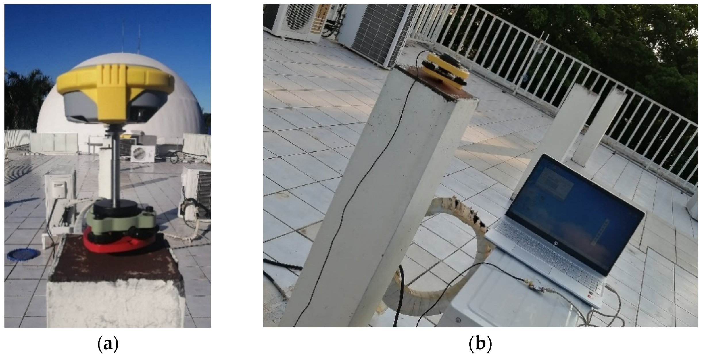
As was mentioned earlier, two observations were made at different dates, but it was considered that the same day and time should be used to maintain similar conditions. First, the campaign with the geodetic receiver (Figure 2a) was carried out on 7 February 2020. Likewise, the observations with the low-cost GNSS receiver (Figure 2b) were carried out on 16 October 2020. In both campaigns, the location was on a stable forced-centering monument located on the roof of the Earth and Space Sciences faculty building, with a clean surrounding antenna environment and optimal weather conditions.

Figure 2.
GNSS receivers used: (a) geodetic order receiver; (b) low-cost GNSS receiver.
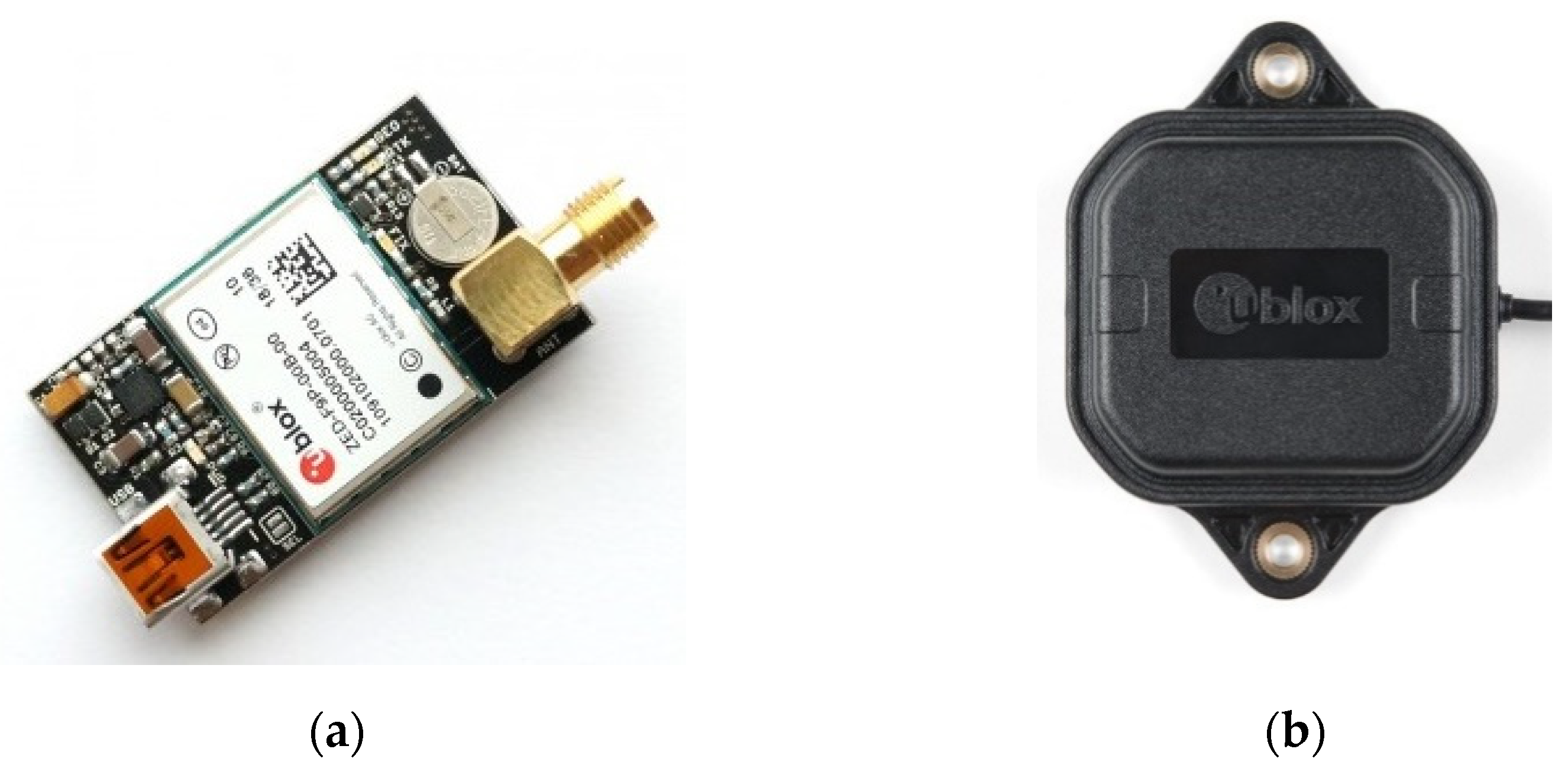
The low-cost GNSS receiver ZED-F9P of the U-Blox series was used for generating the observations (Figure 3a). This low-cost GNSS receiver had 184 channels on the frequencies of GPS: L1C/A, L2C; GLO: L1OF L2OF; GAL: E1B/C, E5b; and BDS: B1I, B2I signals. A convergence time RTK < 10 s, cold start of 24 s and reacquisition time of 2 s were used, along with a navigation and tracking sensibility of 167 dBm, cold start of −148 dBm and hot start of −157 dBm. This was used with a SMA multiband antenna ANN-MB (Figure 3b).
Figure 3.
Equipment used: (a) low-cost GNSS receiver; (b) U-Blox antenna.
With the purpose of testing the impact of different sampling rates on PPP performance using a low-cost GNSS receiver, the sampling rates of each receiver were configured at the highest sampling rate that the equipment allows for. In this sense, the sampling rates were set up to 0.1 and 0.2 s for the low-cost GNSS and geodetic receivers, respectively, with a cut-off angle (elevation mask) of 15°. The duration of the observation was setup for 2 h with the purpose of inspecting the data loss derived from the capability of the registering of the low-cost GNSS receiver. Once the observations were made, the original RINEX of both receivers were decimated with the TEQC software at 0.2, 1, 5, 15 and 30 s for the low-cost GNSS receiver, and likewise, 1, 5, 15 and 30 s for the geodetic receiver. In the same way, the multipath was calculated following the pseudorange multipath approach proposed by [35]. In addition, the signal-to-noise ratio was calculated with the TEQC software for the original sampling rates (0.1 and 0.2 s), with the objective of finding some influence or degradation in the received signal. In addition, in order to analyze the obtained solution derived from the geodetic and low-cost GNSS receivers, the coordinates obtained by using both receivers in both methods were compared to the precise coordinates that were obtained by means of the Trimble Business Center [38] Software.
2.2. PPP-GNSS Data Processing
The new version (version 3) of the Canadian Spatial Reference System PPP service software (CSRS-PPP) was used to process the GNSS data in kinematic and static mode. The main novelty of CSRS-PPP version 3 is the implementation of PPP-AR algorithms [37], which are used to resolve ambiguities for data collected as of 1 January 2018. When a specific set of corrections is applied to the observations of the carrier phase and the parameters of the phase differences are estimated. The ambiguity parameters set up in the PPP filter have an integer nature. Therefore, using sophisticated algorithms, it is possible to identify these integers and restrict their values. When this additional information is added to the solution the accuracy improves. In version 3 of the CSRS-PPP online software the ambiguity resolution is performed on the backward run. This means that epochs are processed first in a chronological order to ensure that all information is available before resolving ambiguities. Then starting with the last successfully processed epoch, ambiguity resolution is attempted. This process is repeated for all epochs in reverse order, that is, from the last to the first epoch. After the backward run is complete, a final back substitution is performed to obtain the final values of all parameters of interest in the process: receiver clocks, tropospheric zenith delays and positions (in kinematic mode) [37].
For the PPP-GNSS data processing, CSRS-PPP can use different types of orbits and clock products such as rapid, ultra rapid and IGS final. For the experiment, the IGS final orbits at 30 s by the International GNSS Service (IGS) were used. According to [21,36,39] the software interpolates at the same sampling rate of the submitted RINEX by using the clock corrections. In the same way, a positioning close to 1 h and 30 min is necessary for kinematic and static mode, respectively. Thus, it allows it to solve the ambiguity of the carrier phase [37]. In this sense, the convergence of the GNSS method is fixed when the accuracy does not present changes or the ambiguities are constant. Table 1 summarizes the options and models implemented in the processing the GNSS data.

Table 1.
Summary of processing options used by CSRS-PPP.
3. Results
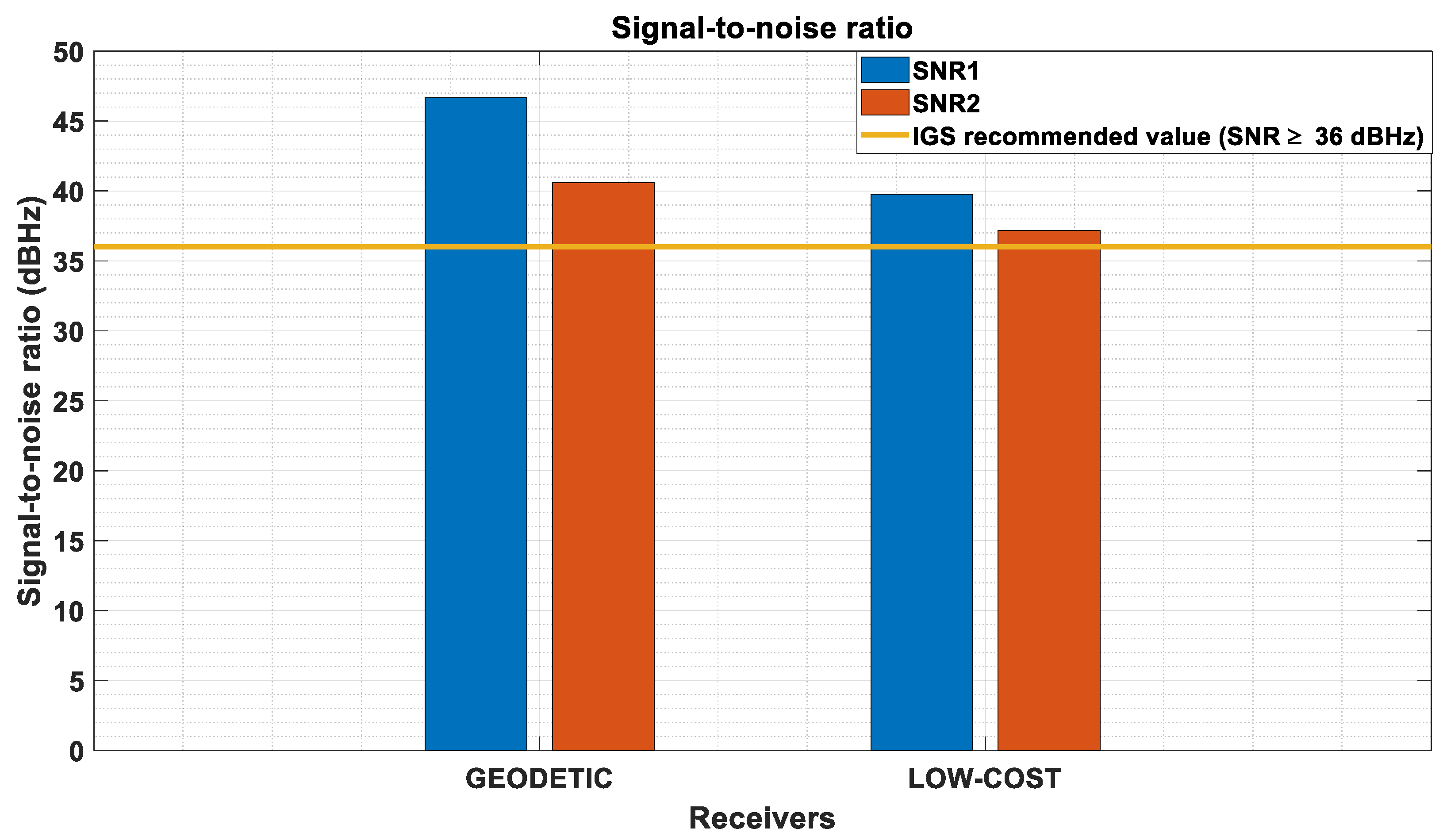
As was mentioned earlier, the calculation of the multipath effect (Figure 4) and signal-to-noise ratio (Figure 5) were made using the TEQC software for the low-cost GNSS and geodetic receivers at 0.1 and 0.2 s, respectively. In [40], it is mentioned that the multipath effect is inversely proportional to the signal-to-noise ratio, this is found in Figure 4 and Figure 5. The low-cost GNSS receiver registered a high value of the multipath effect in both frequencies compared to the IGS recommended value of 0.3 m, this was despite the fact that the low-cost GNSS receiver does not have a polarized antenna to reduce the multipath effect. Nevertheless, a normal value of the multipath effect was registered in general terms compared to the mean global value of the multipath effect in IGS stations [41,42]. Despite the good behavior presented in the signal-to-noise ratio for the low-cost GNSS receiver, the multipath effect obtains high values in contrast to the value recommended by IGS and the geodetic receiver.
Figure 4.
Multipath effect for the low-cost and geodetic GNSS receivers. Yellow line: IGS recommended value (MP < 0.3 m).
Figure 5.
Signal-to-Noise ratio for the low-cost and geodetic GNSS receivers. Yellow line: IGS recommended value (SNR ≥ 36 dBHz).
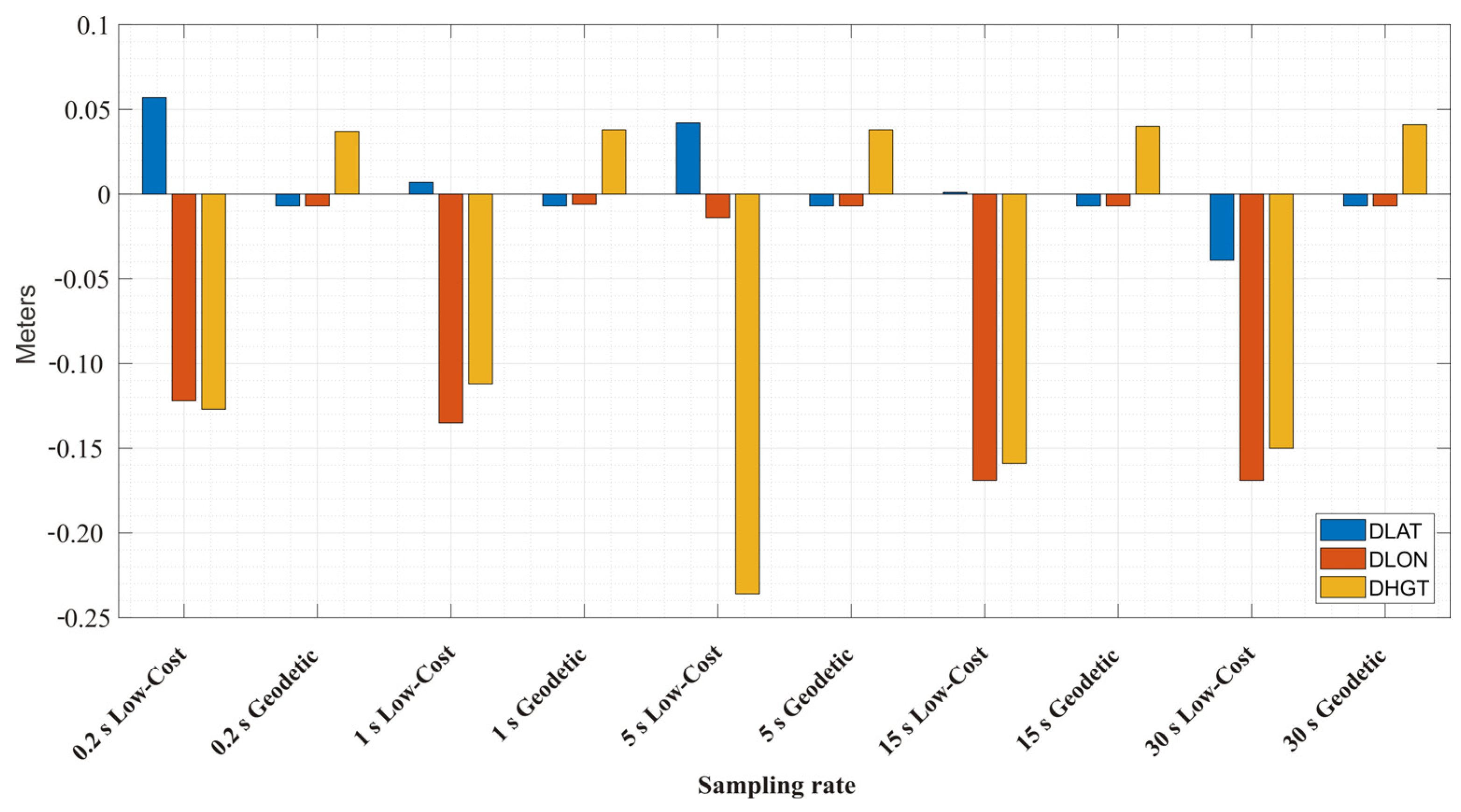
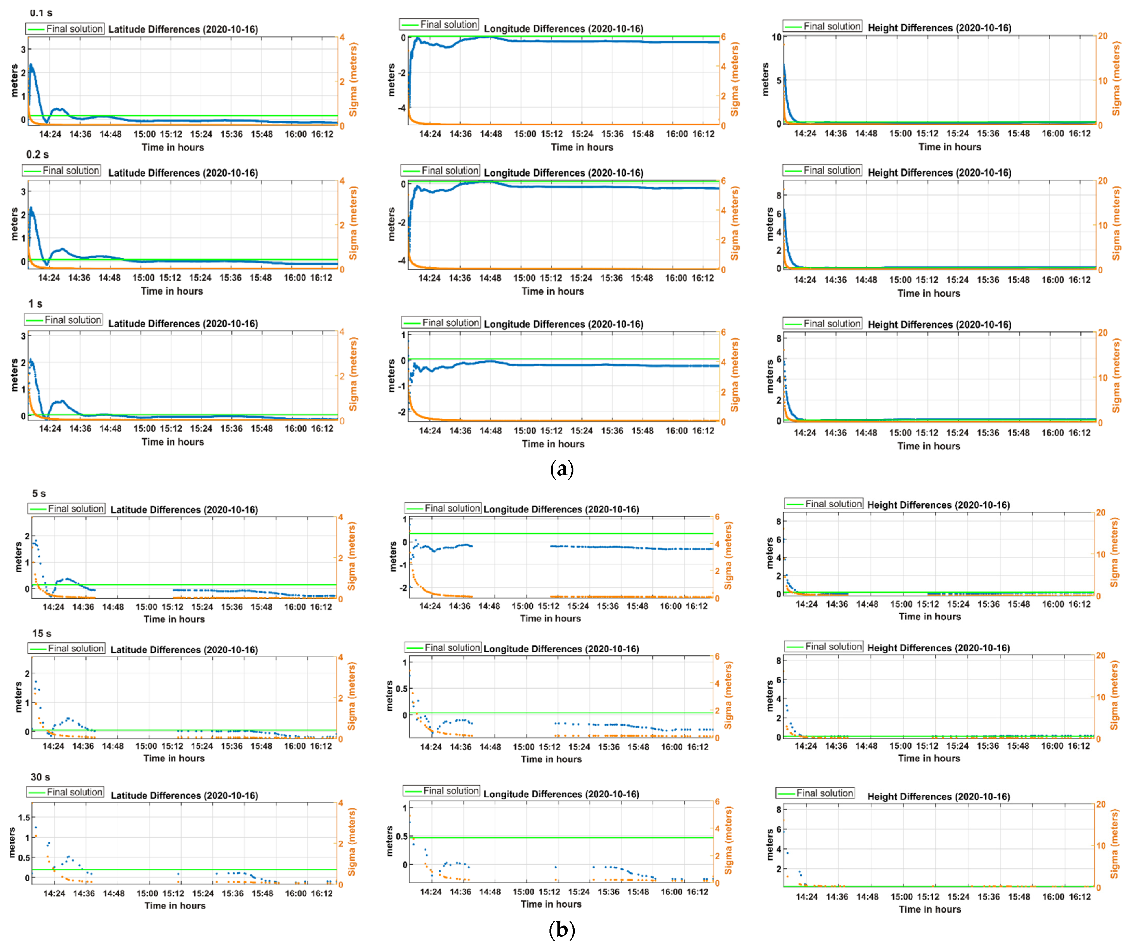
The difference between the estimated and precise coordinates’ position was calculated for each receiver in both modes at different sampling intervals (0.1, 0.2, 1, 5, 15 and 30 s). The values obtained for the low-cost GNSS receiver were small in high frequencies (0.1 and 1 s) for the PPP-static mode, where the height and longitude values presented the greatest difference in the solution. Nonetheless, the obtained values, in comparison with the geodetic receiver, are high (Figure 6). For the low-cost GNSS receiver, the longitude and height obtained solution was constant with the major difference. Regarding the best solution, the low-cost GNSS obtained the best solution in 0.1 and 0.2 s due to the data loss found at low frequencies. In the same way, for the low-cost and geodetic receivers, the difference of the precise and estimated coordinates was constant in all cases. Likewise, the geodetic receiver had the best estimation.
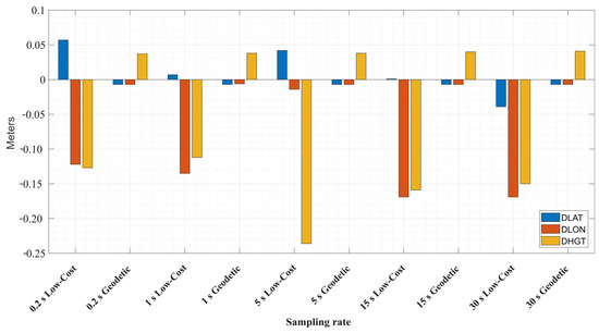
Figure 6.
Difference between estimated and precise coordinates of the low-cost and geodetic receiver by processing with PPP-static mode.
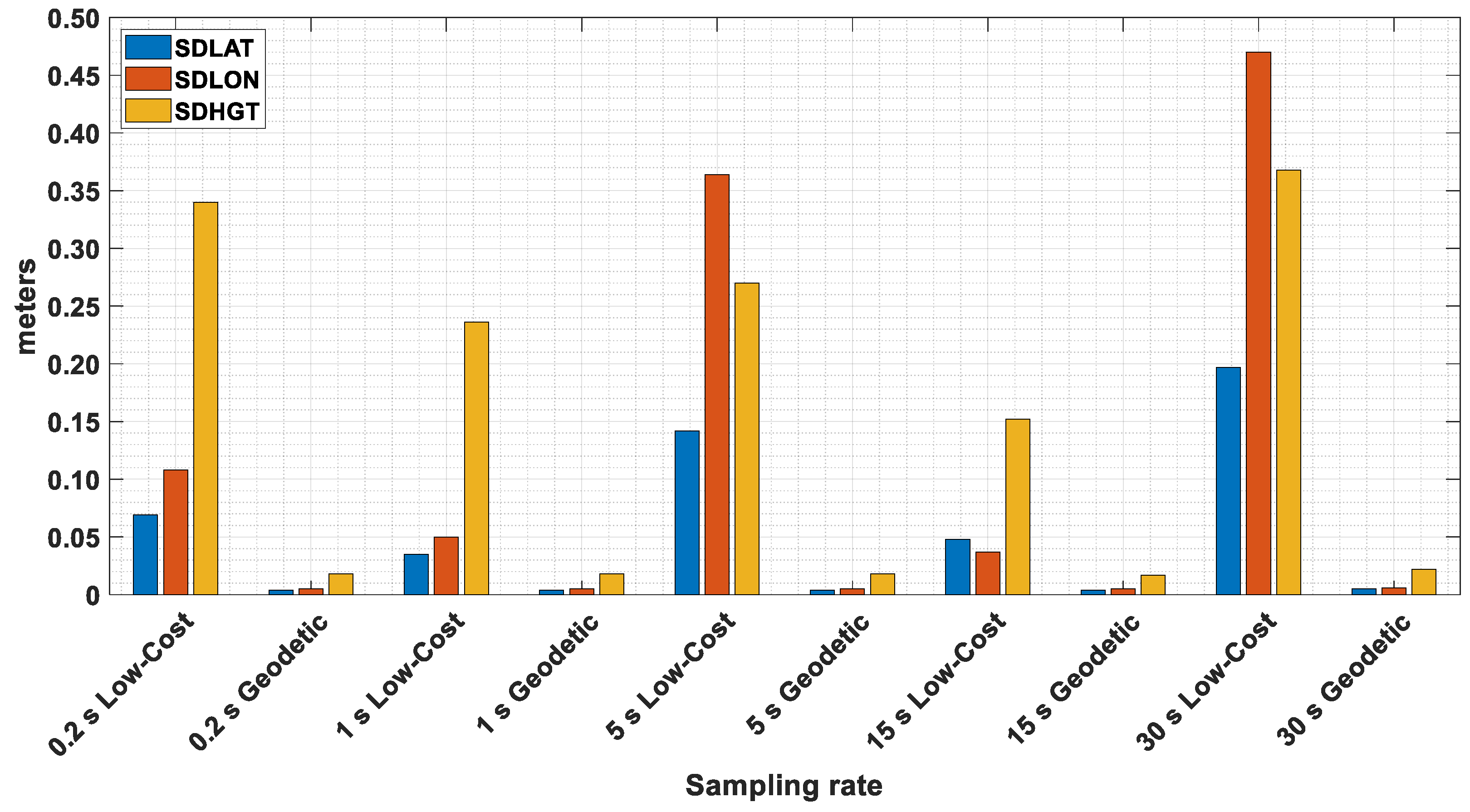
The standard deviation of the estimated positions for each receiver is presented in Figure 7. As was found in Figure 6, the solutions obtained by the geodetic receiver were small and constant. It is found that there is a clear correspondence between the sampling rate and the standard deviation obtained for the low-cost GNSS receiver. In this sense, the standard deviation obtained from the low-cost GNSS receiver is higher compared to the standard deviation from the geodetic receiver, this is clear for all sampling rates. However, the obtained deviation for 1 and 15 s showed the best results, the worst case being at 5 and 30 s. This is because the RINEX file corresponding to the sampling frequency of 5 s had a lower percentage of observations, affecting the processing with the PPP method and the final precision. On the other hand, according to [43] these differences in precision can also be caused by the multipath effect and atmospheric errors (tropospheric and ionospheric). It is also related to the fact that the low-cost GNSS antenna (Figure 3b) does not have an IGS antenna calibration, this affects the obtained solution making it impossible at this point to achieve a mm solution as a relative static method [44].
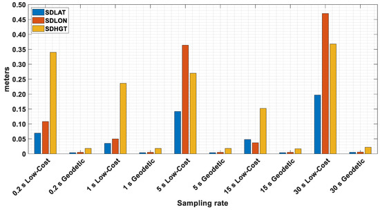
Figure 7.
Standard deviation (95%) of estimated positions of low-cost and geodetic receivers by processing with PPP-static mode.
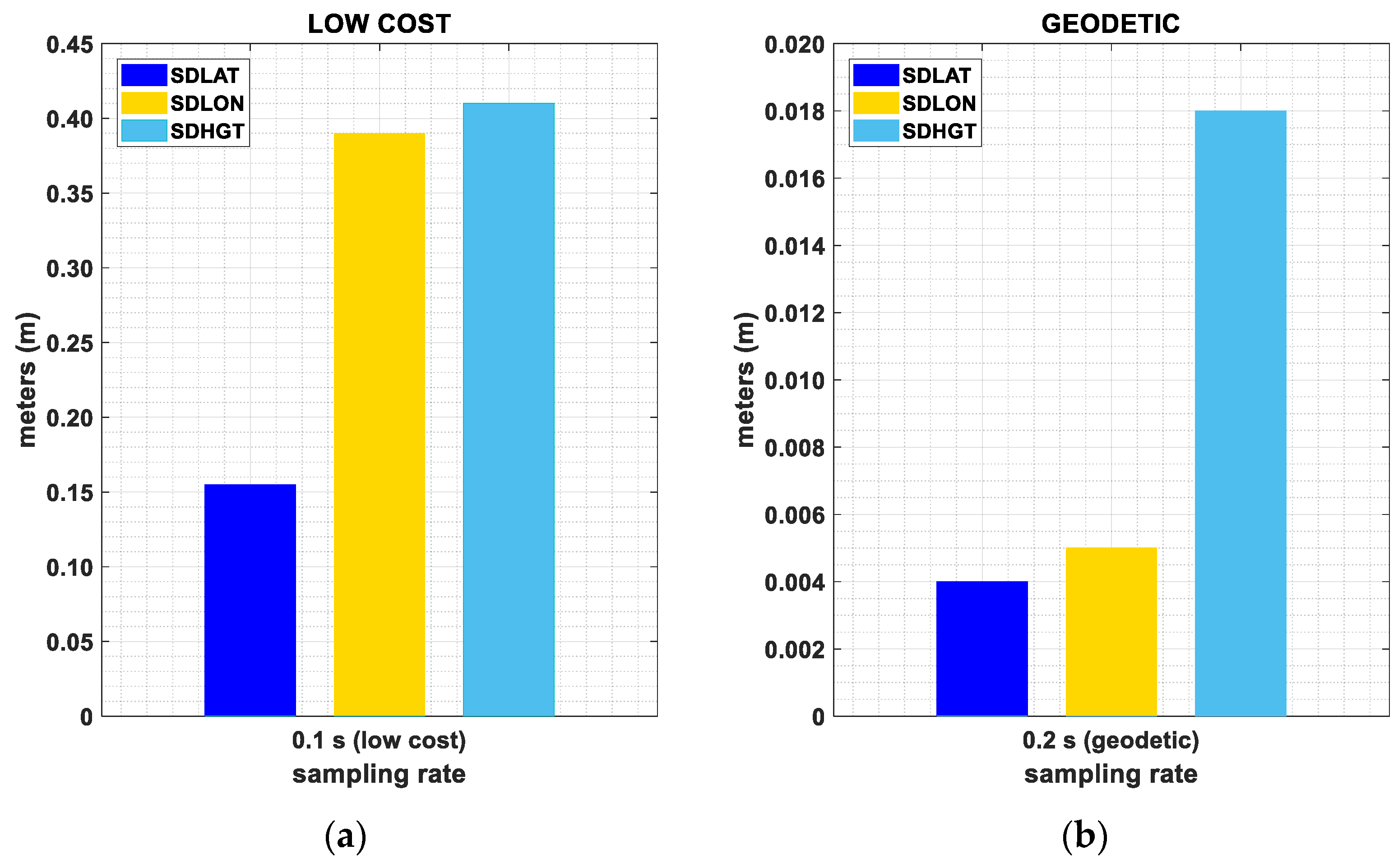
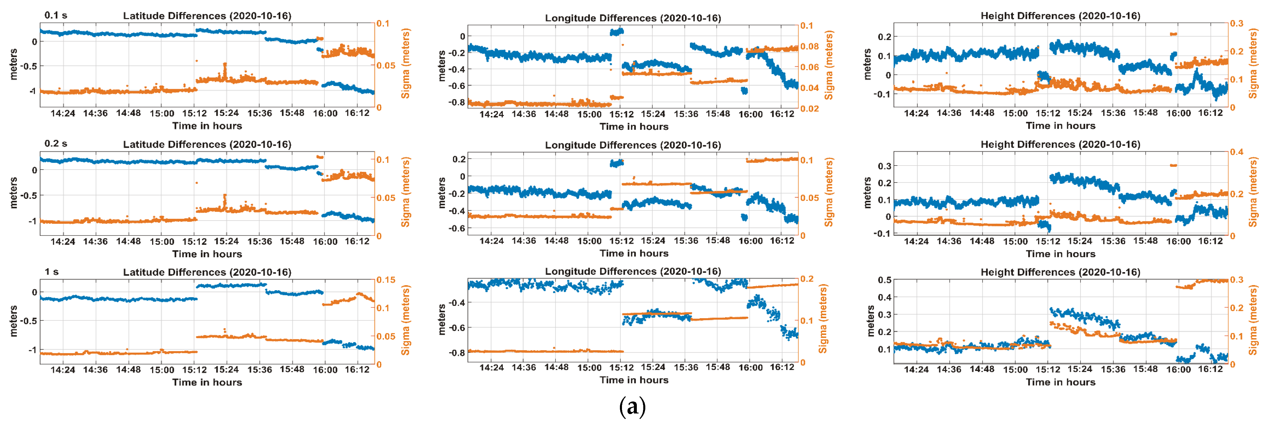
The low-cost and geodetic receivers were set up to the maximum sampling rate they allow, 0.1 and 0.2 s, respectively. In this sense, if the low-cost GNSS receiver was set up to 0.1 s, the obtained values of the standard deviation should be smaller than the geodetic receiver, this was not found. The difference obtained at 0.1 s by the low-cost GNSS receiver is higher compared to the one obtained with geodetic receiver when constant in horizontal and vertical components (Figure 8 and Figure 9).
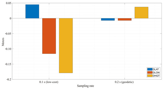
Figure 8.
Difference between estimated and precise position of low-cost and geodetic receivers at 0.1 and 0.2 s respectively, by processing with PPP-static mode.
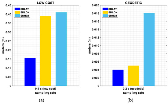
Figure 9.
Standard deviation (95%) of estimated positions by processing with PPP-static mode: (a) low-cost receiver at 0.1 s; (b) geodetic receiver at 0.2 s.
Table 2 presents a summary of the values obtained for the PPP-static mode. For the geodetic receiver, the obtained results are similar in all cases with a precise obtained solution. The low-cost GNSS receiver presented solutions in cm order, nevertheless, at 1 and 15 s the obtained solutions are similar to the solutions from the geodetic receiver.
Table 2.
Differences and Standard deviation obtained at different sampling rates for the PPP-static mode.
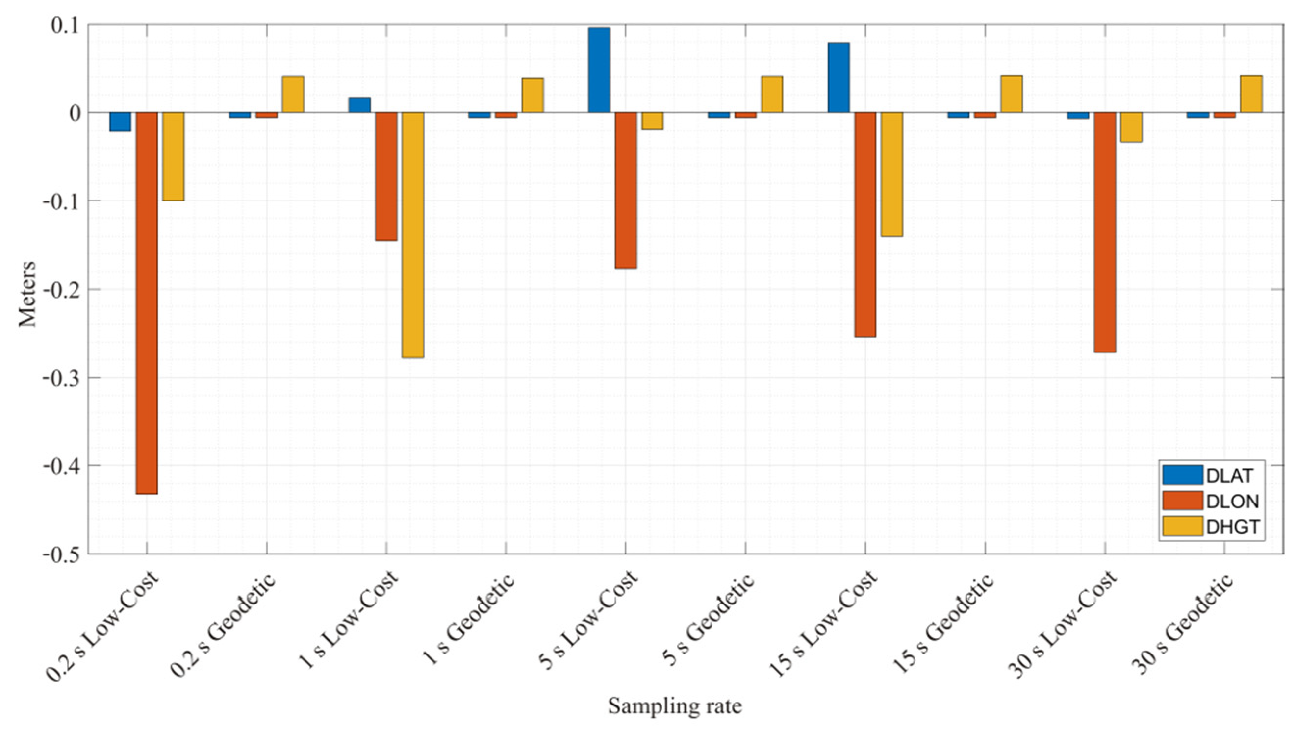
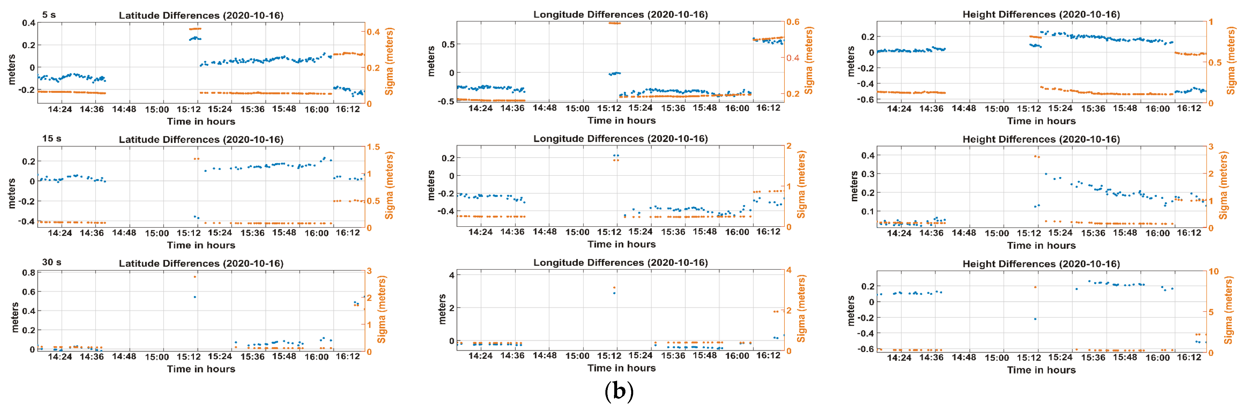
For the kinematic mode, a positive relationship between the observation recording rate and the standard deviation was found (Figure 10). That is, the higher the observation recording rate, the higher the standard deviation values. However, for the difference between the estimates and precise coordinates, the differences obtained are similar and greater than the obtained values from the geodetic receiver. In all cases for the height of the low-cost GNSS receiver the values obtained are higher and are more suitable at 1 s (Figure 11)
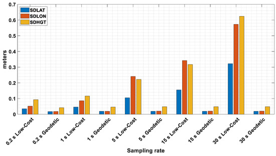
Figure 10.
Standard deviation (95%) of estimated positions of low-cost and geodetic receivers by processing with PPP-kinematic mode.
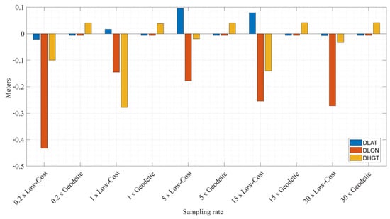
Figure 11.
Difference between estimated and precise positions of low-cost and geodetic receivers by processing with PPP-kinematic mode.
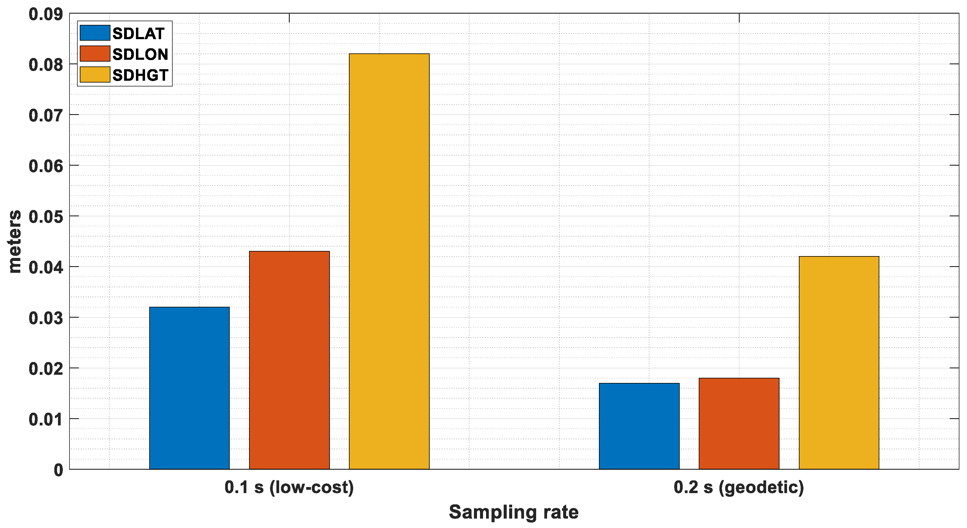
Nonetheless, when the low-cost GNSS receiver was set up to 0.1 s, the results of the difference between the estimated and precise positions (Figure 12) and the standard deviation (Figure 13) are greater than the geodetic receiver.
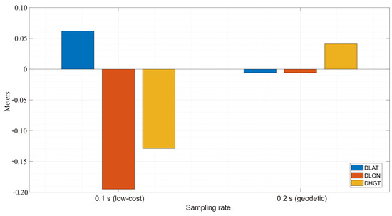
Figure 12.
Difference between estimated and precise positions of low-cost and geodetic receivers at 0.1 and 0.2 s respectively, by processing with PPP-kinematic mode.

Figure 13.
Standard deviation (95%) of estimated positions of low-cost and geodetic receivers at 0.1 and 0.2 s respectively, by processing with PPP-kinematic mode.
The obtained differences of the precise coordinates and estimated coordinates for the low-cost GNSS receiver are higher than the geodetic receiver in all cases (Table 3). In comparison to the static mode, where the behavior of the difference of 1 s is similar to the geodetic receiver, this is not found. In all cases the standard deviation of the low-cost GNSS is greater than the geodetic receiver.
Table 3.
Differences and Standard deviation obtained at different sampling rates for the PPP-kinematic mode.
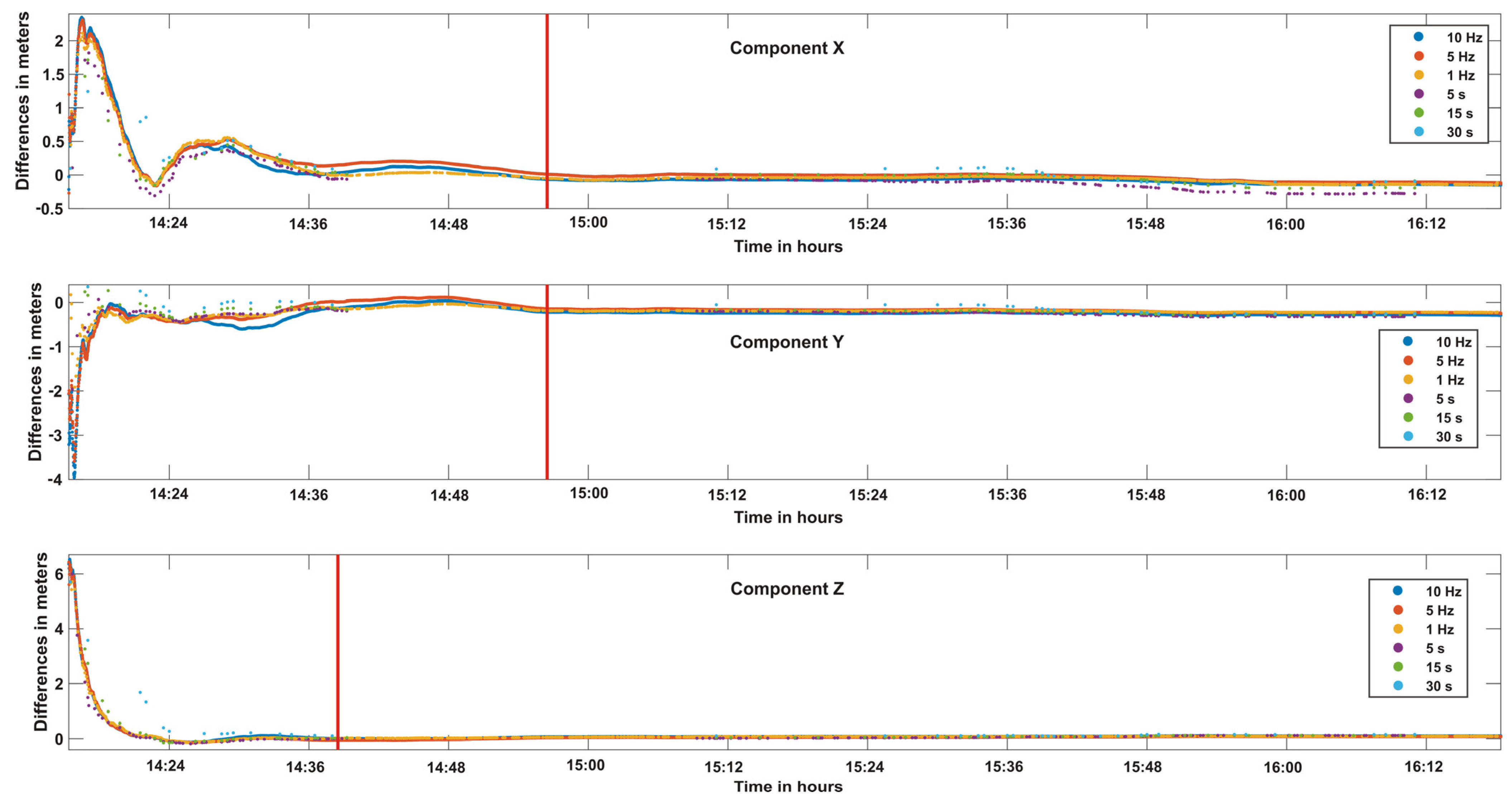
According to [21,43] the convergence time represents the time to reach a stable accuracy level, which depends on many factors such as observation quality, noise level of code observations, user environment, the number and geometry of visible satellites, sampling rate and algorithms. As a result, for measurements obtained from CSRS-PPP for both of the PPP modes, the convergence and the difference of precise (from a previous campaign in static relative mode) and estimated coordinates are analyzed in Figure 14 and Figure 15 with 3D coordinates. As stated by [45] the general rule for the time for the PPP-static solution to converge for a horizontal accuracy (cm) of 5 cm is reached is at 60 min. The PPP-static mode reaches the convergence at 15 min from the first observation (Figure 14), which is seen at each sampling rate for the horizontal and vertical components [46,47]. For the PPP-static mode, the best accuracy and estimated position are achieved at 1, 15 and 0.2 s, compared to 5, 0.1 and 30 s. Notwithstanding, the obtained solution is accurate for all sampling rates. It is clear that for high frequencies, the low-cost GNSS receiver lost data. This affected the accuracy and positioning obtained. Nevertheless, for the high sampling rates, the solution was not affected due to the quantity of observation data.
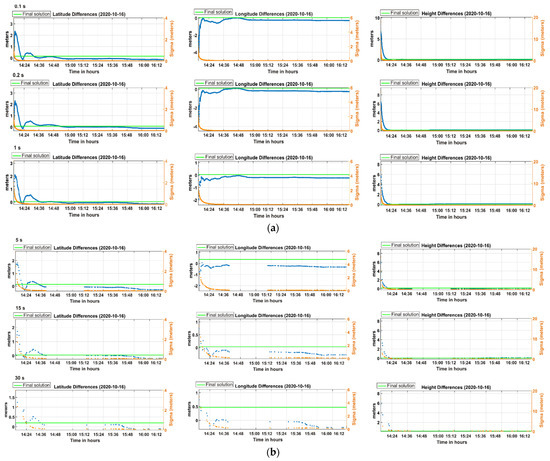
Figure 14.
Low-cost GNSS static mode obtained by processing with CSRS-PPP: (a) sampling rate: 0.1, 0.2 and 1 s; (b) sampling rate: 5, 15 and 30 s.
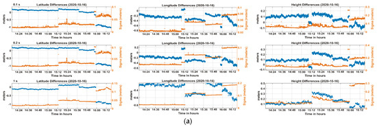
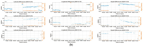
Figure 15.
Low-cost GNSS kinematic mode obtained by processing with CSRS-PPP: (a) sampling rate: 0.1, 0.2 and 1 s; (b) sampling rate: 5, 15 and 30 s.
The PPP-kinematic mode was the most affected mode due to the data loss (Figure 15). This data loss generated an offset in the difference, between estimated and precise positions in the time series. In this sense, the kinematic mode was more affected than the static mode due to the data loss at low frequencies, being more affected at > 5 s sampling rates. The obtained solution at 0.1 s seemed to have linear behaviors as with the rest of the solutions obtained. Nevertheless, as the sampling rates diminished, an offset is seen at the same time in all cases. Apparently, at 30 s the solution obtained was not affected by the data loss due to the linear behavior of the time series.
To evaluate the performance of the PPP-AR convergence time, the differences between the reference coordinates (which were taken as true) and the estimated coordinates obtained by kinematic and static PPP were used. It was considered convergent when the differences reached ± 0.1 m and remained within that limit. The time of convergence was defined as the period from the first epoch to the epoch of convergence (indicated as a red line in Figure 16 and Figure 17). It is observed that the convergence time was more stable in the PPP-static method, however, it was slower compared to PPP-kinematic method. Convergence occurs near 50 min for the horizontal component and near 30 min for the vertical component. This difference in convergence times can be related to the fact that the measurements were carried out on the concrete of a forced-centering monument, which represented greater stability in the vertical component, and in the case of the horizontal it was more affected by the wind currents that hit the antenna.
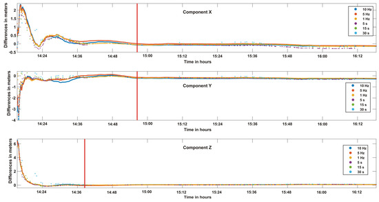
Figure 16.
Convergence time achieved for solutions of the PPP method in static mode.
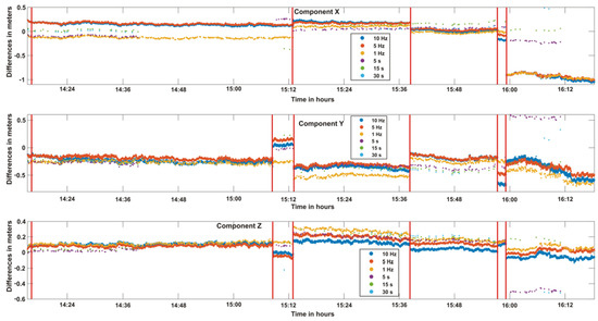
Figure 17.
Convergence time achieved for solutions of the PPP method in kinematic mode.
For the case of the PPP-kinematic method, this presented a greater instability in the convergence time, mainly due to the independent solution method presented by the PPP-kinematic method. The convergence time was reached within the first few minutes of measurement and remained for close to an hour, however, the instability of the solution caused the convergence to be lost and it started to restart for small periods of time. Although convergence was achieved in a shorter time it did not remain constant until the end of the measurement period, as was the case with the PPP-static solution.
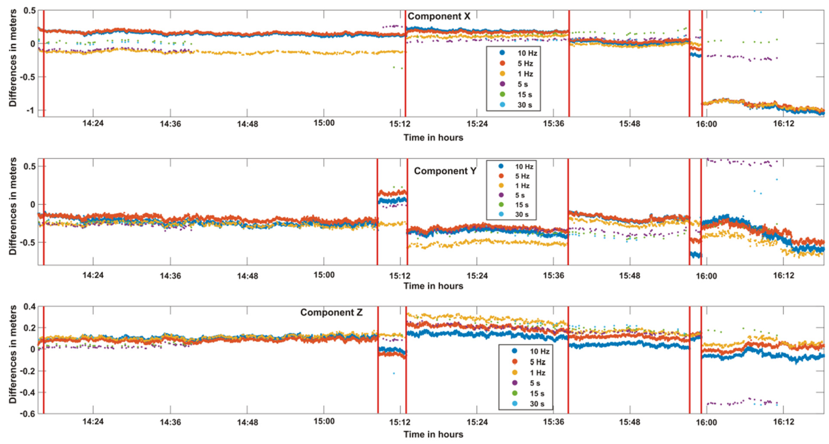
Something new and interesting that should be highlighted in this study is the impact that the measurement interval had in reaching convergence quickly. It is observed in Figure 16 that the highest rate measurement intervals (10, 5 and 1 Hz) are those that had more stability when convergence was reached in static mode. For the case of Figure 17 the same does not occur due to the instability presented by the solutions of the kinematic mode. Of the different measurement intervals, none had a good performance in the 3 components, the 10, 5 and 1 Hz intervals presented good performance in convergence during the first hour but in later times convergence was lost and was reached again only for short periods. Considering the results illustrated in Figure 16 and Figure 17, it is shown that the PPP-static mode had a better performance in converging and staying stable. This is necessary to know when using low-cost GNSS receivers in research areas where the time series represent a physical magnitude of interest, such as displacements, then the static-PPP method must be applied for a real representation of the magnitude.
4. Conclusions
The performance of a multi-constellation low-cost GNSS receiver was evaluated at high sample rates for kinematic- and static-PPP modes. The coordinates of different scenarios were calculated using the online post-processing service CSRS-PPP in its new version of ambiguity resolution PPP-AR. According to the results presented, the following statements can be concluded:
- The low-cost GNSS receiver presented high horizontal accuracy, nevertheless, the vertical component was the most affected. In both components, the obtained results were calculated without considering the low multipath suppression of the antenna of the low-cost GNSS receiver. Likewise, the antenna of the low-cost GNSS receiver did not have an IGS calibration or circular polarized antenna (irregular gain pattern and low multipath suppression), this affected the convergence in some circumstances making it slow (if the antenna is compared with geodetic-grade hardware).
- The results obtained at different sampling rates show that the low-cost GNSS receiver had a better performance (obtained positioning) by using PPP-static mode when the sampling rate was at 1 and 15 s.
- As was presented in Figure 14 and Figure 15, the low-cost GNSS presented data loss at 5, 15 and 30 s, and lower precision at 5 and 30 s. On the other hand, when the data were processed at high frequencies (0.1 and 0.2 s), the precision that was achieved was low in comparison with a 1 s sampling rate.
- An improvement of convergence time is clearly seen (Figure 16 and Figure 17) for the sampling rates of 0.1, 0.2 and 1 s. In the same way, the convergence time was reached at ~50 min in static mode. In the kinematic mode, the convergence time at each interval time was variable and constant with the behavior presented. The convergence was affected by the cycle slips presented or by a high multipath, nevertheless, it was faster than the static mode.
- For the high frequencies a low-cost GNSS receiver is a viable option for obtaining cm solutions if the project allows it.
- According to the results obtained, the low-cost GNSS receiver could be implemented in structural health monitoring systems, mainly due to the centimeter precision achieved in positioning. In addition, it could represent a potential economic alternative by replacing high-cost instruments used in SHM processes.
Finally, the use of low-cost GNSS receivers is suitable for applications such as: monitoring, mapping and positioning. The use of them depends on the characteristics of the project. The impact of the antenna in the low-cost GNSS receivers is one of the most important factors when processing GNSS observations, thus it is important to evaluate the performance and accuracy that can be achieved with a low-cost GNSS receiver with a geodetic grade antenna. Likewise, it is important to analyze the capability of new low-cost GNSS receivers in tracking more signals and other constellations, this could improve the obtained positioning and coverage.
Author Contributions
Conceptualization, R.R.-A. and D.H.-A.; methodology, R.R.-A.; software, R.R.-A., J.R.V.-O. and D.H.-A.; validation, R.R.-A., D.H.-A. and J.R.V.-O.; formal analysis, R.R.-A. and D.H.-A.; investigation, R.R.-A. and J.R.V.-O.; resources, R.R.-A.; data curation, R.R.-A., D.H.-A. and J.R.V.-O.; writing—original draft preparation, R.R.-A.; writing—review and editing, D.H.-A.; visualization, J.L.C.-Z.; supervision, M.E.T.-S.; project administration, D.H.-A.; funding acquisition, R.R.-A. All authors have read and agreed to the published version of the manuscript.
Funding
This research was funded by CONACyT (Consejo Nacional de Ciencia y Tecnología) and the Autonomous University of Sinaloa, in Mexico, grant number CVU: 429125.
Institutional Review Board Statement
Not applicable.
Informed Consent Statement
Not applicable.
Data Availability Statement
All data, models, or code generated or used during the study are available from the corresponding author by request, including raw GPS data, processed GPS data and a quality check of the observations and figures.
Acknowledgments
The authors would also like to thank all anonymous reviewers for their valuable comments, which refined the present work. English corrected by Yuriko Haysu Jacobo Montoya.
Conflicts of Interest
The authors declare no conflict of interest.
References
- Zamora-Maciel, A.; Romero-Andrade, R.; Moraila-Valenzuela, C.R.; Pivot, F. Evaluación de receptores GPS de bajo costo de alta sensibilidad para trabajos geodésicos. Caso de estudio: Línea base geodésica. Cienc. Ergo-Sum 2020, 27, e73. [Google Scholar] [CrossRef]
- Tsakiri, M.; Sioulis, A.; Piniotis, G. The use of low-cost, single-frequency GNSS receivers in mapping surveys. Surv. Rev. 2018, 50, 46–56. [Google Scholar] [CrossRef]
- Poluzzi, L.; Tavasci, L.; Corsini, F.; Barbarella, M.; Gandolfi, S. Low-cost GNSS sensors for monitoring applications. Appl. Geomat. 2019. [Google Scholar] [CrossRef]
- Cina, A.; Piras, M. Performance of low-cost GNSS receiver for landslides monitoring: Test and results. Geomat. Nat. Hazards Risk 2015, 6, 497–514. [Google Scholar] [CrossRef]
- Wang, J.; Yang, N. Economical GNSS Chipset for Application in Structural Health & Deformation Monitoring Solution. In Proceedings of the Smart Surveyors for Land and Water Management—Changes in a New Reality Virtually in the Netherlands, FIG. The Netherlands, (virtually) Online. 21–25 June 2021; pp. 21–25. Available online: https://fig.net/resources/proceedings/fig_proceedings/fig2021/papers/ts06.2/TS06.2_yang_10933.pdf (accessed on 20 August 2021).
- Garrido-Carretero, M.S.; de Lacy-Pérez de los Cobos, M.C.; Borque-Arancón, M.J.; Ruiz-Armenteros, A.M.; Moreno-Guerrero, R.; Gil-Cruz, A.J. Low-cost GNSS receiver in RTK positioning under the standard ISO-17123-8: A feasible option in geomatics. Measurement 2019, 137, 168–178. [Google Scholar] [CrossRef]
- Guo, L.; Jin, C.; Liu, G. Evaluation on measurement performance of low-cost GNSS receivers. In Proceedings of the 2017 3rd IEEE International Conference on Computer and Communications (ICCC), Chengdu, China, 13–16 December 2017; pp. 1067–1071. [Google Scholar] [CrossRef]
- Romero-Andrade, R.; Cabanillas-zavala, J.L.; Hernández-andrade, D.; Trejo-soto, M.E.; Monjardin-armenta, S.A. Análisis Comparativo Del Posicionamiento GNSS Utilizando Receptor De Bajo Costo U-Blox De Doble Frecuencia Para Aplicaciones Topógrafo-Geodésicas. Eur. Sci. J. 2020, 16, 289–312. [Google Scholar] [CrossRef]
- Tsakiri, M.; Sioulis, A.; Piniotis, G. Compliance of low-cost, single-frequency GNSS receivers to standards consistent with ISO for control surveying. Int. J. Metrol. Qual. Eng. 2017, 8, 11. [Google Scholar] [CrossRef] [Green Version]
- Romero-Andrade, R.; Zamora-Maciel, A.; Uriarte-Adrián, J.D.J.; Pivot, F.; Trejo-Soto, M.E. Comparative analysis of precise point positioning processing technique with GPS low-cost in different technologies with academic software. Measurement 2019, 136, 337–344. [Google Scholar] [CrossRef]
- Lu, L.; Ma, L.; Wu, T.; Chen, X. Performance analysis of positioning solution using low-cost single-frequency u-blox receiver based on baseline length constraint. Sensors 2019, 19, 4352. [Google Scholar] [CrossRef] [Green Version]
- Hamza, V.; Stopar, B.; Ambrožič, T. Testing Multi-Frequency Low-Cost GNSS Receivers for Geodetic Monitoring Purposes. Sensors 2020, 20, 4375. [Google Scholar] [CrossRef]
- Hofmann-Wellenhof, B.; Lichtenegger, H.; Wasle, E. GNSS Global Navigation Satellite System GPS, GLONASS, Galileo and More; Springer: Vienna, Austria; New York, NY, USA, 2008; ISBN 9783211730126. [Google Scholar]
- Ferhat, G.; Malet, J.-P.; Ulrich, P. Evaluation of different processing strategies of Continuous GPS (CGPS) observations for landslide monitoring. In Proceedings of the European Geosciences Union General Assembly 2015, Vienna, Austria, 12–17 April 2015; Volume 17, p. 10582. [Google Scholar]
- Hamza, V.; Stopar, B.; Sterle, O. Testing the performance of multi-frequency low-cost gnss receivers and antennas. Sensors 2021, 21, 2029. [Google Scholar] [CrossRef] [PubMed]
- Odolinski, R.; Teunissen, P.J.G. Best integer equivariant estimation: Performance analysis using real data collected by low-cost, single- and dual-frequency, multi-GNSS receivers for short- to long-baseline RTK positioning. J. Geod. 2020, 94, 91. [Google Scholar] [CrossRef]
- Vazquez-Ontiveros, J.R.; Vazquez-becerra, G.E.; Quintana, J.A.; Carrion, J.; Guzman-acevedo, G.M.; Gaxiola-camacho, J.R. Implementation of PPP-GNSS measurement technology in the probabilistic SHM of bridge structures. Measurement 2020, 20, 108677. [Google Scholar] [CrossRef]
- Anderle, R.J. Point positioning concept using precise ephemeris. In Proceedings of the Satellite Doppler Positioning, Las Cruces, NM, USA, 12–14 October 1976; Volume 1, pp. 47–75. [Google Scholar]
- Zumberge, J.F.; Heftin, M.B.; Jefferson, D.; Watkins, M.M.; Webb, F.H. Precise point positioning for the efficient and robust analysis of GPS data from large networks. J. Geophys. Res. 1997, 102, 5005–5017. [Google Scholar] [CrossRef] [Green Version]
- Luo, X.; Gu, S.; Lou, Y.; Xiong, C.; Chen, B.; Jin, X. Assessing the performance of GPS precise point positioning under different geomagnetic storm conditions during solar cycle 24. Sensors 2018, 18, 1784. [Google Scholar] [CrossRef] [Green Version]
- Erol, S.; Alkan, R.M.; Ozulu, İ.M.; Ilçi, V. Impact of different sampling rates on precise point positioning performance using online processing service. Geo-Spat. Inf. Sci. 2020, 24, 302–312. [Google Scholar] [CrossRef]
- Alkan, R.; İlçİ, V. Accuracy Comparison of PPP Using GPS-only and Combined GPS + GLONASS Satellites in Urban Area: A Case Study in Çorum. J. Arab. Inst. Navig. 2015, 32, 7–12. [Google Scholar]
- Xin, S.; Geng, J.; Guo, J.; Meng, X. On the Choice of the Third-Frequency Galileo Signals in Accelerating PPP Ambiguity Resolution in Case of Receiver Antenna Phase Center Errors. Remote Sens. 2020, 12, 1315. [Google Scholar] [CrossRef] [Green Version]
- Yigit, C. Ozer Experimental assessment of post-processed kinematic Precise Point Positioning method for structural health monitoring. Geomat. Nat. Hazards Risk 2016, 7, 360–383. [Google Scholar] [CrossRef] [Green Version]
- Xu, P.; Shi, C.; Fang, R.; Liu, J.; Niu, X.; Zhang, Q.; Yanagidani, T. High-rate precise point positioning (PPP) to measure seismic wave motions: An experimental comparison of GPS PPP with inertial measurement units. J. Geod. 2013, 87, 361–372. [Google Scholar] [CrossRef]
- Bahadur, B.; Nohutcu, M. Impact of observation sampling rate on Multi-GNSS static PPP performance. Surv. Rev. 2020, 53, 206–215. [Google Scholar] [CrossRef]
- Manzini, N.; Orcesi, A.; Thom, C.; Brossault, M.A.; Botton, S.; Ortiz, M.; Dumoulin, J. Performance analysis of low-cost GNSS stations for structural health monitoring of civil engineering structures. Struct. Infrastruct. Eng. 2020. [Google Scholar] [CrossRef]
- Psychas, D.; Verhagen, S.; Teunissen, P.J.G. Precision analysis of partial ambiguity resolution-enabled PPP using multi-GNSS and multi-frequency signals. Adv. Space Res. 2020, 66, 2075–2093. [Google Scholar] [CrossRef]
- Tang, X.; Li, X.; Roberts, G.W.; Hancock, C.M.; de Ligt, H.; Guo, F. 1 Hz GPS satellites clock correction estimations to support high-rate dynamic PPP GPS applied on the Severn suspension bridge for deflection detection. GPS Solut. 2019, 23, 28. [Google Scholar] [CrossRef]
- Geng, J.; Guo, J.; Meng, X.; Gao, K. Speeding up PPP ambiguity resolution using triple-frequency GPS/BeiDou/Galileo/QZSS data. J. Geod. 2020, 123, 6. [Google Scholar] [CrossRef] [Green Version]
- Banville, S.; Geng, J.; Loyer, S.; Schaer, S.; Springer, T.; Strasser, S. On the interoperability of IGS products for precise point positioning with ambiguity resolution. J. Geod. 2020, 94, 10. [Google Scholar] [CrossRef]
- Pan, Z.; Chai, H.; Kong, Y. Integrating multi-GNSS to improve the performance of precise point positioning. Adv. Space Res. 2017, 60, 2596–2606. [Google Scholar] [CrossRef]
- Teunissen, P.J.G. GNSS Precise Point Positioning. In Position, Navigation, and Timing Technologies in the 21st Century; John Wiley Sons Ltd.: Hoboken, NJ, USA, 2020; pp. 503–528. ISBN 9781119458449. [Google Scholar]
- Gurtner, W. Innovation: Rinex The Receiver Independent Exchange Format. GPS World 1994, 5, 48–53. [Google Scholar]
- Estey, L.H.; Meertens, C.M. TEQC: The multi-purpose toolkit for GPS/GLONASS data. GPS Solut. 1999, 3, 42–49. [Google Scholar] [CrossRef]
- Tétreault, P.; Kouba, J.; Héroux, P.; Legree, P. CSRS-PPP: An internet service for GPS user access to the Canadian Spatial Reference frame. Geomatica 2005, 59, 17–28. [Google Scholar]
- CSRS-PPP. The Canadian Spatial Reference System, Natural Resources Canada. Available online: https://webapp.geod.nrcan.gc.ca/geod/tools-outils/ppp-update.php (accessed on 1 December 2020).
- Trimble Business Center; Trimble Navigation Limited: Dayton, OH, USA, 2017; ISBN 1937233944.
- Mireault, Y.; Tétreault, P.; Lahaye, F.; Héroux, P.; Kouba, J. Online Precise Point Positioning: A new, timely service from Natural Resources Canada. GPS World 2008, 19, 59–64. [Google Scholar]
- Kamatham, Y. Estimation, analysis and prediction of multipath error for static GNSS applications. In Proceedings of the 2018 Conference on Signal Processing And Communication Engineering Systems (SPACES), Vijayawada, India, 4–5 January 2018; pp. 62–65. [Google Scholar] [CrossRef]
- Hernández-Andrade, D.; Romero-Andrade, R.; Cabanillas-Zavala, J.L.; Ávila-Cruz, M.; Trejo-Soto, M.E.; Vega-Ayala, A. Análisis de calidad de las observaciones GPS en estaciones de operación continua de libre acceso en México. Eur. Sci. J. 2020, 16, 332. [Google Scholar] [CrossRef]
- García-Armenteros, J.A. Monitorización Y Control De Calidad De Las Estaciones De La Red Cgps Topo-Iberia-UJA. Eur. Sci. J. 2020, 16, 1. [Google Scholar] [CrossRef]
- Yigit, C.O.; El-mowafy, A.; Dindar, A.A.; Bezcioglu, M.; Tiryakioglu, I. Investigating Performance of High-Rate GNSS-PPP and PPP-AR for Structural Health Monitoring: Dynamic Tests on Shake Table. J. Surv. Eng. 2021, 147, 05020011. [Google Scholar] [CrossRef]
- Wen, Q.; Geng, J.; Li, G.; Guo, J. Precise point positioning with ambiguity resolution using an external survey-grade antenna enhanced dual-frequency android GNSS data. Measurement 2020, 157, 107634. [Google Scholar] [CrossRef]
- Choy, S.; Bisnath, S.; Rizos, C. Uncovering common misconceptions in GNSS Precise Point Positioning and its future prospect. GPS Solut. 2017, 21, 13–22. [Google Scholar] [CrossRef]
- Abou-Galala, M.; Rabah, M.; Kaloop, M.; Zidan, Z.M. Assessment of the accuracy and convergence period of Precise Point Positioning. Alex. Eng. J. 2018, 57, 1721–1726. [Google Scholar] [CrossRef]
- Galala, M.; Rabah, M.; Zidan, Z. Assessment of the Accuracy and Convergence Period of Precise Point Positioning. Bull. Fac. Eng. Mansoura Univ. 2020, 41, 1–5. [Google Scholar] [CrossRef]


Publisher’s Note: MDPI stays neutral with regard to jurisdictional claims in published maps and institutional affiliations. |
© 2021 by the authors. Licensee MDPI, Basel, Switzerland. This article is an open access article distributed under the terms and conditions of the Creative Commons Attribution (CC BY) license (https://creativecommons.org/licenses/by/4.0/).