A Common Framework for Developing Robust Power-Flow Methods with High Convergence Rate

Featured Application

This work proposes a common framework for developing robust Power-Flow solvers that may find multiple applications in power system analysis tools.

Abstract

This paper presents a novel Power-Flow solution paradigm based on the structure of the members of the Runge–Kutta family. Solution approaches based on the introduced solution paradigm are intrinsically robust and can achieve high-order convergences rates. It is demonstrated that some well-known Power-Flow solution methods are in fact special cases of the developed framework. Explicit and embedded formulations are discussed, and two novel solution methodologies based on the Explicit Heun and Embedded Heun–Euler’s methods are developed. The introduced solution techniques are validated in the EU PEGASE systems, considering different starting points and loading levels. Results show that the developed methods are quite reliable and efficient, outperforming other robust and standard methodologies. On the basis of the results obtained, we can affirm that the introduced solution paradigm constitutes a promising framework for developing novel Power-Flow solution techniques.

1. Introduction

1.1. Motivation

The Power-Flow (PF) is one of the main computational tools in power system analysis. It solves the nonlinear model of a power system for a given power generation/consumption profile. Nowadays, the Newton–Raphson (NR) is still the most widely used technique for solving the nonlinear equations involved in the PF problem. This is because of its simplicity, easy codification in standard programming languages, acceptable robustness, and quadratic convergence. These features typically bring superior characteristics with respect to (w.r.t.) other conventional PF solvers.

The PF problems are customary categorized as well or ill-conditioned. Conventionally, a PF problem is said to be ill-conditioned when its solution by using standard techniques such as NR is hardly reachable [1]. This has supposed an important barrier for the wide application of Newton-like techniques; nevertheless, this issue has not been very problematic due to most PF cases being well-conditioned. However, ill-conditioned cases are becoming more frequent [2]. Solving these kinds of problems is still challenging due to the difficulties showed by standard methods or the low degree of efficiency manifested by most of the available robust PF solution techniques. In this context, developing novel efficient and robust PF solution approaches is still interesting, relevant, and demanding.

1.2. Literature Review

PF solutions in ill-conditioned cases have been widely studied since Iwamoto and Tamura developed a robust step size-based solution methodology in [3]. For each iteration of this methodology, an optimal factor is calculated that modifies the Newton’s increment vector so that it evolves, reducing the sum of squares of the residual. This approach, although quite robust, is very inefficient because the solution is approached very slowly [4]. In addition, this methodology is only suitable when the PF equations are formulated in rectangular coordinates [3]; however, polar formulations have been explored [5].

Since NR considers a first-order truncation of the Taylor series truncation of PF equations, its accurate and reliability can be enhanced by using a second-order expansion. This approach arises in the so-called second-order PF solution methods, which have not been widely used in industry applications due to the expensive calculation of the Hessian matrix. The author of [6] proposed an elegant variant of the second-order methodologies that avoids the explicit computation of the Hessian matrix.

Milano proposed a common framework between the NR-based solution of the PF and the Forward Euler methodology in [1]. On the basis of this analogy, it is established that any explicit numerical method can be adapted for developing robust PF solution techniques. This idea has been widely exploited by the authors in several references [7,8,9,10,11]. The implicit formulation of this paradigm has been recently proposed in [12].

In [2,13], a dynamic solution paradigm for solving the PF was proposed. It takes advantage of the computational integration routines, so that a widely convergent methodology is obtained. However, its computational cost is still very expensive, which limits its application in realistic large-scale systems.

The Levenberg method has been exploited for PF analysis in several references [14,15,16]. Although these techniques might be very efficient and convergence is normally ensured (at least in the least squares sense), the obtained value may not correspond with the explicit solution of the PF equations [14], which might bring accuracy issues.

Recently, several efforts have been made in order to adapt the Holomorphic Embedding Method to the solution of the PF equations (see e.g., [17] and references therein). The Holomorphic Embedding Method represents an infinite number of formulations, each one with different numerical properties. An alternative point of view was proposed by the authors in [18]. It takes advantage of the homotopy theorem which, in combination with other efficient numerical techniques, arises in a novel family of robust and efficient PF solution methods.

1.3. Contributions and Paper Organization

This paper arises from a careful study of the work developed in [6]. As commented, this reference proposes a second-order methodology that avoids the explicit computation of the Hessian matrix. This technique was called NR with Jacobian adjustments (NRJ). The authors observed that NRJ could be also interpreted as the adaptation of the Explicit Midpoint method to the PF analysis, but in a different way compared with the Midpoint PF solution procedure considered in [1,10]. Keeping this in mind, any other member of the Runge–Kutta family [19] could be adapted in a similar way to the PF problem, so that a huge variety of novel PF solution methods can be developed based on the introduced solution framework. This idea, although it presents some similitudes with the work developed in [1], brings two main advantages with respect to this reference:

• Methodologies developed in this work are intrinsically robust, which means, unlike those in [1,7,8,9,10,11,12], it is not necessary to include a discrete step size in the formulation to improve their convergence properties.
• Methodologies based on the introduced solution paradigm achieve, at least, a quadratic convergence rate, which makes them competitive with standard solvers such as NR.

The latter point is especially relevant since PF solution techniques based on the proposed solution framework might be also high order Newton-like methods, which is reflected in the superior convergence characteristics in comparison with NR and other robust PF methods. In this paper, Explicit and Embedded formulations of the developed solution paradigm are discussed, and two novel robust and efficient PF solution techniques with cubic order of convergence are developed. In order to validate the developed methodologies, they have been tested in several realistic systems based on the European Transmission system.

The remainder of this paper is organized as follows. Section 2 introduces the developed common framework for developing high-order robust PF solution methods. Two novel solution techniques based on the introduced solution paradigm are developed in Section 3. Several numerical experiments and results are presented in Section 4. Finally, the paper is concluded in Section 5.

2. The Developed Solution Framework for PF Analysis

2.1. Analogy between NRJ and the Explicit Midpoint Method

Let us consider the PF problem in polar coordinates as a set of nonlinear equations as follows:

$$g\left(\mathit{x}\right) = 0$$

(1)

where $g:{\mathbb{R}}^n⟼{\mathbb{R}}^n$ are the PF equations and $\mathit{x}\in {\mathbb{R}}^n$ is the PF state vector. Due to strong nonlinearities in (1), its solution must be achieved by using iterative techniques. The most popular one in PF analysis is NR, which is performed as follows:

$${\mathit{x}}^{\left(k+1\right)} = {\mathit{x}}^{\left(k\right)}-{\left[g^{\prime }\left({\mathit{x}}^{\left(k\right)}\right)\right]}^{-1}g\left({\mathit{x}}^{\left(k\right)}\right)$$

(2)

where ${\left[*\right]}^{-1}:{\mathbb{R}}^n\mapsto {\mathbb{R}}^n$ is the inverse operator, the superscript denotes the $k^{t\mathbf{h}}$ iteration of the iterative procedure, and $g^{\prime }\in {\mathbb{R}}^{n\times n}$ is the Jacobian matrix of the PF equations, which is formed by the first partial derivatives of $g$ w.r.t. $\mathit{x}$. In contrast to (2), NRJ poses a two-step iterative scheme for solving the set in Equation (1) described by:

$$\left\{\begin{array}{c}{\mathit{y}}_2^{\left(k\right)} = {\mathit{x}}^{\left(k\right)}-\frac{1}{2}{\left[g^{\prime }\left({\mathit{x}}^{\left(k\right)}\right)\right]}^{-1}g\left({\mathit{x}}^{\left(k\right)}\right) \\ {\mathit{x}}^{\left(k+1\right)} = {\mathit{x}}^{\left(k\right)}-{\left[g^{\prime }\left({\mathit{y}}_2^{\left(k\right)}\right)\right]}^{-1}g\left({\mathit{x}}^{\left(k\right)}\right) \end{array}\right..$$

(3)

In [10], the Explicit Midpoint rule [19] was exploited for solving the PF equations on the basis of the Continuous Newton’s principle. This technique poses a two-stage iterative solver, which is given by the mapping in (4).

$$\left\{\begin{array}{c}{\mathit{y}}_2^{\left(k\right)} = {\mathit{x}}^{\left(k\right)}+\left(\frac{1}{2}·∆t\right)f\left({\mathit{x}}^{\left(k\right)}\right)\\ {\mathit{x}}^{\left(k+1\right)} = {\mathit{x}}^{\left(k\right)}+∆tf\left({\mathit{y}}_2^{\left(k\right)}\right) \end{array}\right.$$

(4)

where $∆t\in {\mathbb{R}}^{+}$ is the step size (or truncation) and $f:{\mathbb{R}}^n⟼{\mathbb{R}}^n$ is given by:

$$f\left(\mathit{x}\right) = -{\left[g^{\prime }\left(\mathit{x}\right)\right]}^{-1}g\left(\mathit{x}\right).$$

(5)

Further insight on mappings (3) and (4) reveals a clear analogy between these two solvers. In fact, the iterative map (3) could be rewritten as follows:

$$\left\{\begin{array}{c}{\mathit{y}}_2^{\left(k\right)} = {\mathit{x}}^{\left(k\right)}+\frac{1}{2}\mathbf{h}\left({\mathit{x}}^{\left(k\right)},{\mathit{x}}^{\left(k\right)}\right) \\ {\mathit{x}}^{\left(k+1\right)} = {\mathit{x}}^{\left(k\right)}+\mathbf{h}\left({\mathit{y}}_2^{\left(k\right)},{\mathit{x}}^{\left(k\right)}\right) \end{array}\right.$$

(6)

where the step size has vanished and the auxiliary function $\mathbf{h}:{\mathbb{R}}^n⟼{\mathbb{R}}^n$ is defined by:

$$\mathbf{h}\left(\mathit{y},\mathit{x}\right) = -{\left[g^{\prime }\left(\mathit{y}\right)\right]}^{-1}g\left(\mathit{x}\right).$$

(7)

The analogy described above reveals that NRJ and the Explicit Midpoint rule are actually equivalent mappings. Keeping this in mind, NRJ may be seen as the application of the Explicit Midpoint method for solving the function $\mathbf{h}$, whereas the different methodologies proposed in [1,10] are devoted to solving $f$. In the same way, NR could be assimilated as the direct application of the Explicit Euler methodology for solving (7).

2.2. The Novel Family of Robust PF Techniques

In the previous section, we showed that NR and NRJ can be seen as the application of the Explicit Euler and Midpoint techniques for solving (7). This analogy suggests that any other member of the family of Explicit Runge–Kutta methods can be adapted to be applied to the PF problem. Similar to the generic form of the Runge–Kutta methods (e.g., see [10] (Equation (11)), we could develop a generic form for the application of this family of numerical methods to the PF problem, as follows:

$$\left\{\begin{array}{c}{\mathit{y}}_2^{\left(k\right)} = {\mathit{x}}^{\left(k\right)}+a_{\left.2\right|1}\mathbf{h}\left({\mathit{x}}^{\left(k\right)},{\mathit{x}}^{\left(k\right)}\right) \\ {\mathit{y}}_3^{\left(k\right)} = {\mathit{x}}^{\left(k\right)}+a_{\left.3\right|1}\mathbf{h}\left({\mathit{x}}^{\left(k\right)},{\mathit{x}}^{\left(k\right)}\right)+a_{\left.3\right|2}\mathbf{h}\left({\mathit{y}}_2^{\left(k\right)},{\mathit{x}}^{\left(k\right)}\right) \\ ⋮\\ {\mathit{y}}_p^{\left(k\right)} = {\mathit{x}}^{\left(k\right)}+a_{\left.p\right|1}\mathbf{h}\left({\mathit{x}}^{\left(k\right)},{\mathit{x}}^{\left(k\right)}\right)+{\displaystyle {\displaystyle \sum }_{i = 2}^p}\left\{a_{\left.p\right|i}\mathbf{h}\left({\mathit{y}}_i^{\left(k\right)},{\mathit{x}}^{\left(k\right)}\right)\right\}\\ {\mathit{x}}^{\left(k+1\right)} = {\mathit{x}}^{\left(k\right)}+b_1\mathbf{h}\left({\mathit{x}}^{\left(k\right)},{\mathit{x}}^{\left(k\right)}\right)+{{\displaystyle \sum }}_{i = 2}^m\left\{b_i\mathbf{h}\left({\mathit{y}}_i^{\left(k\right)},{\mathit{x}}^{\left(k\right)}\right)\right\}\end{array}\right.$$

(8)

where the $a$ and $b \mathrm{values}\in \mathbb{R}$. In essence, these parameters are introduced to copy the standard structure of the Runge–Kutta methods, which are broadly defined by the total number of stages involved ($p$), the value of the elements of the Runge–Kutta matrix ($a$ values) and weights ($b$ values) [19]. Conventionally, the Runge–Kutta methods are presented by their so-called Butcher tableaus [19] (p. 95), which succinctly collects all the necessary information to completely define a Runge–Kutta technique, as follows:

$$\mathit{A} = \left[\begin{array}{cccc}0& & & \\ a_{\left.2\right|1}& a_{\left.2\right|2}& \begin{array}{cc}& \end{array}\\ ⋮& & \ddots & \\ a_{\left.p\right|1}& \cdots & a_{\left.p\right|p-1}& a_{\left.p\right|p}\end{array}\right]\in {\mathbb{R}}^{p\times p}$$

(9)

$$\mathit{b} = \left[b_1,b_2,\dots ,b_m\right]\in {\mathbb{R}}^m.$$

(10)

It is worth mentioning that (9) is lower triangular, since we are dealing with explicit Runge–Kutta formulas (the implicit formulation of (8), although possible, may be computationally expensive, since it would require the factorization of the inverse of (7) [1]). In addition, it is worth noting that nodes [19] are not included in the formulation developed in this paper. This is because the application of the Runge–Kutta formulas to PF analysis is developed from the assimilation of the set of equations (1) as an autonomous set of differential equations. In such formulations, the nodes of a numerical method lack importance [19].

One can note that (8) can be adapted to any Explicit Runge–Kutta formula. At this point, readers can easily check that both NR and NRJ are actually special cases of (8). Thus, for NR, one has:

$$\mathit{A} = \left[\begin{array}{cc}0& 0\\ 1& 0\end{array}\right], \mathit{b} = \left[1, 0\right].$$

(11)

While NRJ is fully described by:

$$\mathit{A} = \left[\begin{array}{cc}0& 0\\ 1/2& 0\end{array}\right], \mathit{b} = \left[0, 1\right].$$

(12)

Interested readers can easily check in the vast literature that (11) and (12) correspond with the Runge–Kutta matrix and weight vectors of the Explicit Euler and Midpoint techniques, respectively.

2.3. Embedded Formulation

The solution paradigm established in the previous section allows considering any explicit numerical method for developing robust PF solution techniques. However, not only explicit numerical integration techniques are available in the literature. The Embedded Runge–Kutta techniques arise as an alternative of Explicit methods. Such methodologies allow accurately estimating the local truncation error of a single step and properly adapting the step size to obtain high accuracy [19]. In this case, due to the step size having vanished in the developing formulation, its ability to estimate the local truncation error lacks importance; nonetheless, it is still relevant to rewrite (8) into its Embedded counterpart as follows:

$$\left\{\begin{array}{c}{\mathit{y}}_2^{\left(k\right)} = {\mathit{x}}^{\left(k\right)}+a_{\left.2\right|1}\mathbf{h}\left({\mathit{x}}^{\left(k\right)},{\mathit{x}}^{\left(k\right)}\right) \\ {\mathit{y}}_3^{\left(k\right)} = {\mathit{x}}^{\left(k\right)}+a_{\left.3\right|1}\mathbf{h}\left({\mathit{x}}^{\left(k\right)},{\mathit{x}}^{\left(k\right)}\right)+a_{\left.3\right|2}\mathbf{h}\left({\mathit{y}}_2^{\left(k\right)},{\mathit{x}}^{\left(k\right)}\right)\\ ⋮ \\ \begin{array}{c}{\mathit{y}}_p^{\left(k\right)} = {\mathit{x}}^{\left(k\right)}+a_{\left.p\right|1}\mathbf{h}\left({\mathit{x}}^{\left(k\right)},{\mathit{x}}^{\left(k\right)}\right)+{\displaystyle {\displaystyle \sum }_{i = 2}^p}\left\{a_{\left.p\right|i}\mathbf{h}\left({\mathit{y}}_i^{\left(k\right)},{\mathit{x}}^{\left(k\right)}\right)\right\} \\ {\widehat{\mathit{x}}}^{\left(k\right)} = {\mathit{x}}^{\left(k\right)}+b_1^{*}\mathbf{h}\left({\mathit{x}}^{\left(k\right)},{\mathit{x}}^{\left(k\right)}\right)+{{\displaystyle \sum }}_{i = 2}^m\left\{b_i\mathbf{h}\left({\mathit{y}}_i^{\left(k\right)},{\mathit{x}}^{\left(k\right)}\right)\right\} \end{array}\\ {\mathit{x}}^{\left(k+1\right)} = {\widehat{\mathit{x}}}^{\left(k\right)}+\left(b_1-b_1^{*}\right)\mathbf{h}\left({\mathit{x}}^{\left(k\right)},{\mathit{x}}^{\left(k\right)}\right)+{{\displaystyle \sum }}_{i = 2}^m\left\{\left(b_i-b_i^{*}\right)\mathbf{h}\left({\mathit{y}}_i^{\left(k\right)},{\mathit{x}}^{\left(k\right)}\right)\right\}\end{array}\right.$$

(13)

where $b^{*}$ values $\in \mathbb{R}$. Unlike paradigm (8), each weight in (13) is described by a pair of parameters ($b$ and $b^{*}$). In this case, two numerical methods are nested, each contributing their own characteristic weights. In numerical analysis, this arrangement is very useful for achieving higher accuracy, while in our case, these parameters have been introduced just for copying the standard structure of the Embedded Runge–Kutta formulas [19] (p. 204). Thus, instead of directly calculating the value of the state vector for the $k+1$ iteration through a single step arrangement, formulation (13) firstly calculates an approximation of the state vector $\widehat{\mathit{x}}$ that is posteriorly refined by means of other numerical methods defined by the $b^{*}$ values (see [20] for further details). This way, any PF solver based on the developed paradigm (13) could be defined by two matrixes as follows:

$$\mathit{A} = \left[\begin{array}{cccc}0& & & \\ a_{\left.2\right|1}& a_{\left.2\right|2}& \\ ⋮& a_{\left.p\right|1}& \cdots & \\ a_{\left.p\right|1}& \ddots & a_{\left.p\right|p-1}& a_{\left.p\right|p}\end{array}\right]\in {\mathbb{R}}^{p\times p}$$

(14)

$$\mathit{B} = \left[\begin{array}{c}{b}_1^{*},b_2^{*},\dots ,b_m^{*}\\ b_1, b_2,\dots ,b_m\end{array}\right]\in {\mathbb{R}}^{2\times m}.$$

(15)

It is worth noting that unlike the techniques developed in [1,7,8,9,10,11,12], any truncation of the Newton’s increment vector based on the influence of the step size is considered in the developed solution frameworks. It means that the developed solution techniques are (as shown in Section 4) intrinsically robust. This point is relevant, since the influence of the step size vanishes, facilitating its codification and application in industry tools.

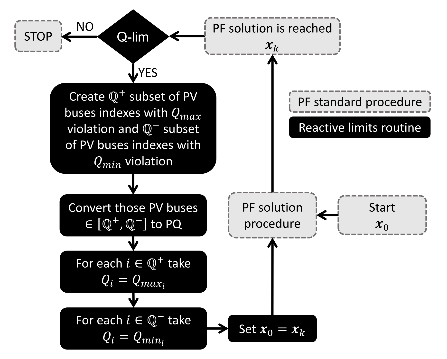
2.4. Handling Equipment Limits

Handling equipment limits (such as those imposed by e.g., generators, on-load tap changers, etc.) is an important topic in PF analysis. The developed solution frameworks (8) and (13) do not directly take into account these limits; however, they could be easily incorporated. In this case, we have considered the same strategy used in [21]. Particularizing to the case of reactive limits in generation units, this approach consists of checking the reactive limits of all generators after a PF solution is calculated. Then, if any limit has been violated, those buses are converted to PQ, and the violated limit is taken as the reactive power injection of this new PQ bus. Then, taking the obtained solution as a starting point, the process is repeated until a feasible solution is reached. This strategy is described in the flowchart of Figure 1. One should note that other control parameters such as transformer tap changers can be taken into account using similar strategies. It is worth mentioning that the developed solution framework is versatile enough to easily incorporate other strategies, such as that described in [2].

2.5. Stability of the Developed Solution Paradigms

In order to study the stability of the mappings (8) and (13), let us introduce the following definition:

Definition 1:

Hyperbolic points: a fixed point ${\mathit{x}}^{*}$ of a map $\mathbf{G} :\mathit{C}\subset {\mathbb{R}}^n\to {\mathbb{R}}^n$ is hyperbolic, if the Jacobian of the equation $\dot{\mathbf{G}} = \mathbf{G}\left(\mathit{x}\right)-\mathit{x}$ at ${\mathit{x}}^{*}$ has no eigenvalues with a zero real part. In addition, ${\mathit{x}}^{*}$ is asymptotically stable if all the eigenvalues of the Jacobian of $\dot{\mathbf{G}}$ at ${\mathit{x}}^{*}$ have a modulus ≤ 1. A hyperbolic point can be:

• Sink: if all the eigenvalues of the Jacobian of $\dot{\mathbf{G}}$ have a negative real part.
• Source: if at least one of the eigenvalues of the Jacobian of $\dot{\mathbf{G}}$ has a positive real part.

Contrarily, a fixed point is said to be unstable if it is not stable.

By Definition 1, one requires a PF solution (i.e., ${\mathit{x}}^{*}$ such that $g\left({\mathit{x}}^{*}\right) = 0$) to be asymptotically stable. In addition, we desire from ${\mathit{x}}^{*}$ to be a sink. By using definition 1, we can study the numerical stability of the developed solution frameworks, which is performed in the following lemma.

Lemma 1:

a solution of the PF equations (i.e., ${\mathit{x}}^{*}$ such that $g\left({\mathit{x}}^{*}\right) = 0$) is a sink for the nonlinear solution paradigms (8) and (13), if ${\displaystyle {{\displaystyle \sum }}_{i = 1}^m}{b}_i\ge 0$ and ${\displaystyle {{\displaystyle \sum }}_{i = 1}^m}\left(b_i-b_i^{*}\right)\ge 0$, respectively.

Proof of Lemma 1.

By differentiating (7) with respect $\mathit{x}$ one obtains:

$${\nabla }_{\mathit{x}}\mathbf{h} = -{\nabla }_{\mathit{x}}{\left[g^{\prime }\left(\mathit{y}\right)\right]}^{-1}g\left(\mathit{x}\right)-{\left[g^{\prime }\left(\mathit{y}\right)\right]}^{-1}{g}^{\prime }\left(\mathit{x}\right).$$

(16)

One can easily check that at an equilibrium point (i.e., ${\mathit{x}}^{*}$ such that $g\left({\mathit{x}}^{*}\right) = 0$), the developed solution paradigms (8) and (13) take the form:

$${\left.{\mathit{y}}_i\right|}_{{\mathit{x}}^{*}} = {\mathit{x}}^{*}, \forall i.$$

(17)

Substituting (17) into (16), one obtains:

$${\left.{\nabla }_{\mathit{x}}\mathbf{h}\right|}_{{\mathit{x}}^{*}} = -{\nabla }_{\mathit{x}}{\left[g^{\prime }\left({\mathit{x}}^{*}\right)\right]}^{-1}g\left({\mathit{x}}^{*}\right)-{\left[g^{\prime }\left({\mathit{x}}^{*}\right)\right]}^{-1}{g}^{\prime }\left({\mathit{x}}^{*}\right) = -\mathit{I}$$

(18)

where $\mathit{I}\in {\mathbb{R}}^{n\times n}$ is the identity matrix. Then, one can replace (18) into the differential equation associated with the mapping (8) obtaining:

$${\left.{\nabla }_{\mathit{x}}\left({\mathit{x}}^{\left(k+1\right)}-{\mathit{x}}^{\left(k\right)}\right)\right|}_{{\mathit{x}}^{*}} = -{{\displaystyle \sum }}_{i = 1}^m\left\{b_i\mathit{I}\right\}.$$

(19)

While for the paradigm (13), one has:

$${\left.{\nabla }_{\mathit{x}}\left({\mathit{x}}^{\left(k+1\right)}-{\widehat{\mathit{x}}}^{\left(k\right)}\right)\right|}_{{\mathit{x}}^{*}} = -{{\displaystyle \sum }}_{i = 1}^m\left\{\left(b_i-b_i^{*}\right)\mathit{I}\right\}.$$

(20)

Equations (19) and (20) show that at the equilibrium point, all the eigenvalues of the Jacobian of the differential equations associated with the developed solution paradigms do not have imaginary parts. In addition, their real parts are equal to $-{\displaystyle {{\displaystyle \sum }}_{i = 1}^m}\left\{b_i\right\}$ in the case of (8) and $-{\displaystyle {{\displaystyle \sum }}_{i = 1}^m}\left\{b_i-b_i^{*}\right\}$ for the mapping (13). Therefore, the equilibrium point ${\mathit{x}}^{*}$ is asymptotically stable for the paradigm (8) if:

$${\displaystyle {{\displaystyle \sum }}_{i = 1}^m}{b}_i\ge 0.$$

(21)

While for the mapping (13), the following inequality must hold:

$${\displaystyle {\displaystyle \sum }_{i = 1}^m}\left(b_i-b_i^{*}\right)\ge 0$$

(22)

 □

3. Developed PF Solvers

For the sake of exemplifying, we have developed two novel robust techniques based on the introduced solution paradigms defined by (8) and (13).

Firstly, we have taken the Explicit Heun’s method for solving (7), which brings the following iterative procedure for solving the PF equations:

$$\left\{\begin{array}{c}{\mathit{y}}_2^{\left(k\right)} = {\mathit{x}}^{\left(k\right)}-\mathbf{h}\left({\mathit{x}}^{\left(k\right)},{\mathit{x}}^{\left(k\right)}\right) \\ {\mathit{x}}^{\left(k+1\right)} = {\mathit{x}}^{\left(k\right)}-\frac{1}{2}\left[\mathbf{h}\left({\mathit{x}}^{\left(k\right)},{\mathit{x}}^{\left(k\right)}\right)+\mathbf{h}\left({\mathit{y}}_2^{\left(k\right)},{\mathit{x}}^{\left(k\right)}\right)\right]\end{array}\right..$$

(23)

On the other hand, taking the developed formulation (13) and considering the Embedded Heun–Euler method, the following iterative procedure for solving the PF equations is introduced:

$$\left\{\begin{array}{c}\begin{array}{c}{\mathit{y}}_2^{\left(k\right)} = {\mathit{x}}^{\left(k\right)}-\mathbf{h}\left({\mathit{x}}^{\left(k\right)},{\mathit{x}}^{\left(k\right)}\right) \\ {\widehat{\mathit{x}}}^{\left(k\right)} = {\mathit{x}}^{\left(k\right)}-\left(1-0\right)\mathbf{h}\left({\mathit{x}}^{\left(k\right)},{\mathit{x}}^{\left(k\right)}\right) \end{array}\\ {\mathit{x}}^{\left(k+1\right)} = {\widehat{\mathit{x}}}^{\left(k\right)}-\left(1-\frac{1}{2}\right)\mathbf{h}\left({\mathit{x}}^{\left(k\right)},{\mathit{x}}^{\left(k\right)}\right)-\left(0-\frac{1}{2}\right)\mathbf{h}\left({\mathit{y}}_2^{\left(k\right)},{\mathit{x}}^{\left(k\right)}\right)\end{array}\right..$$

(24)

The developed PF solution techniques require two matrix evaluations (and factorizations) along with a function evaluation each iteration. In addition, they achieve cubic convergence (see Appendix A). As a result of these features, one can guess that the developed techniques are more efficient than those presented in [1,9,10]. It is worth remarking on the outstanding features of the developed methods since, besides their intrinsic robustness characteristics that are empirically proved by results (see Section 4), they present a high convergence rate. These two characteristics are very difficult to be found simultaneously in a PF solver.

For the sake of summarizing,

Table 1. Definition of some PF solvers based on the developed solution paradigms using matrix/vector notation.

Solver	Analogy	$\mathit{A}$	$\mathit{b}$ $\mathbf{or}\mathit{B}$
NR (2)	Explicit Euler	$\left[\begin{array}{cc}0& 0\\ 1& 0\end{array}\right]$	$\left[1, 0\right]$
NRJ (6)	Explicit Midpoint	$\left[\begin{array}{cc}0& 0\\ 1/2& 0\end{array}\right]$	$\left[0, 1\right]$
(23)	Explicit Heun	$\left[\begin{array}{cc}0& 0\\ 1& 0\end{array}\right]$	$\left[1/2, 1/2\right]$
(24)	Embedded Heun–Euler	$\left[\begin{array}{cc}0& 0\\ 1& 0\end{array}\right]$	$\left[\begin{array}{cc}1/2& 1/2\\ 1& 0\end{array}\right]$

shows the $\mathit{A}$ matrix and $\mathit{b}$ vectors (or $\mathit{B}$ matrix), of NR, NRJ, and the developed PF solution methods (23) and (24). To complete the section, the PF solution procedure using any of the developed techniques is summarized in Algorithm 1 using pseudocode. This algorithm aims to serve as a guidance for easily implementing the developed solvers in standard programming languages such as MATLAB or C. It is worth mentioning that this algorithm can be adapted to NR and NRJ by just replacing Equation (23) or (24) by (2) or (6), respectively. In addition, we have considered the failure of our algorithms when they do not converge in a predetermined number of iterations $k^{\max }$. This situation usually indicates divergence. In the pseudocode of Algorithm (1), the parameter tolerance makes mention of a predefined value beyond which it is assumed that the calculated solution is accurate enough and the algorithm may be determined successfully convergent. It is worth noting that the iterative nonlinear algorithms are unable to calculate the exact solution as in the case of linear systems; therefore, it is customary to establish a threshold for determining when the correct solution is sufficiently approached. Typical values for convergence tolerances in PF studies are fixed below ${10}^{-4}$ [7,8,9,10,11].

Algorithm 1: Developed PF solution techniques

1: Set iteration counter: $k\leftarrow 0$

2: Initial variable guess: $x^{\left(k\right)}\leftarrow x^{\left(0\right)}$

3: # Iterations

4: while $\Vert g{\left(x^{\left(k\right)}\right)\Vert }_{\infty }>tolerance$ do

5:  Solve (23) # or (24)

6:  Update iteration counter: $k\leftarrow k+1$

7:  if $k\ge k^{\max }$ then

8:   break # fail

9:  end if

10: end do

11: return solution $x^{\left(k\right)}$

4. Numerical Experiments

A variety of numerical experiments have been carried out in order to compare the performance of the developed techniques with other well-known PF solvers.

The developed Explicit Heun and Embedded Heun–Euler solution approaches (Equations (23) and (24), respectively) are compared with the standard NR, the Reverse Bulirsch–Stoer solver (RBS) [9], the Newton–Raphson with Jacobian adjustments (NRJ) [6], and the implicit implementation of the Continuous Newton’s method using the Backward-Euler technique (BEM) [12]. In this latter case, we have used the implementation labelled ‘Implicit-Continuous Newton Method with approximated Hessian and the solution of the inner loop is approximated by its first iteration (ICNM-J1)’ in reference [12].

All simulations have been obtained using Matpower [22] and running on a 3 GHz Intel Core i5-8500 personal laptop (8.00 GB RAM). In all experiments, a convergence tolerance of ${10}^{-5}$ and $k^{\max } = 2000$ have been considered. The maximum number of iterations was tuned high enough to only discriminate the divergence cases. In order to avoid the impact of parallel computational activities, the reported execution times have been calculated taken as the average values of 1000 simulations. To determine the goodness of the solutions calculated, they have been compared with those obtained using NR and the default starting point provided in Matpower. Thereby, if both solutions differ more than 0.1 per unit (p.u.), the obtained solution is considered inaccurate.

4.1. Studied Systems

Five realistic systems based on the European Transmission system from the EU PEGASE project have been considered [23,24]. These meshed networks range from 89 to 13,569 buses, thus comprising a wide variety of scenarios. For the sake of self-sufficiency,

Table 2. Main characteristics of the studied systems.

System	Buses	Branches	Generators	Load		$\mathit{n}$
				MW	MVar
89-bus	89	210	12	5727.9	1374.9	165
1354-bus	1354	1991	260	73,059.7	13,401.4	2447
2869-bus	2869	4582	510	132,437.3	29,007.8	5227
9241-bus	9241	16,049	1445	312,354.1	73,581.6	17,036
13659-bus	13,659	20,467	4092	381,431.9	98,523.4	23,225

reports the main characteristics of the studied systems. A starting point, built by modifying the correct solution of the studied cases using a Gaussian distribution and a determined standard deviation, has been considered. These starting guesses aim at emulating a real situation in which an available system solution is used for initializing the PF analysis. In our opinion, this approach is more realistic than the conventional flat start, because the iterative algorithm starts from an explicit solution of the system; this way, the starting point could be considered more “natural” than a flat guess. We call the reader’s attention toward a similar approach that has been also considered in [12]. In order to enable the reproducibility of the results reported, the studied systems with the considered starting points can be found in [25].

4.2. Convergence Rates for Base Cases

Our first test is devoted to comparing the convergence rates for base cases.

Table 3. Total iterations for base cases.

Method	89-Bus	1354-Bus	2869-Bus	9241-Bus	13659-Bus
NR	Fail	Fail	Fail	Fail	Fail
RBS	13	13	Fail	Fail	Fail
BEM	14	13	13	14	14 *
NRJ	7	5	5	Fail	Fail
Equation (23)	5	5	5	6	6
Equation (24)	5	5	5	6	6

* Low convergence solution.

provides the total iterations for the studied systems. As observed, NR failed in all studied cases, which denotes a high degree of ill-conditioning [1]. RBS only successfully solved the 89- and 1354-bus cases, while NRJ failed in the 9241- and 13659-bus cases. On the other hand, BEM converged to the low voltage solution in the 13659-bus system. The developed PF solvers successfully solved all the studied cases. In addition, our proposals usually required less iterations than the remainder of the methodologies. These results serve to empirically demonstrate the robustness characteristic and efficiency salient features of the developed PF solvers.

4.3. Convergence Rates with Reactive Limits

Next, we explore the ability of the tested methods to solve the studied systems with reactive limits. To do that, the strategy described in Section 2.4. has been implemented within the considered algorithms.

Table 4. Total iterations with reactive limits.

Method	89-Bus	1354-Bus	2869-Bus	9241-Bus	13659-Bus
NR	Fail	Fail	Fail	Fail	Fail
RBS	13	32	Fail	Fail	Fail
BEM	14	32	40	42	25 *
NRJ	7	8	9	Fail	Fail
Equation (23)	5	8	9	10	7
Equation (24)	5	8	9	10	7

* Low convergence solution.

reports the total iterations for the studied systems. Similar conclusions as for the base case can be extracted for this scenario.

4.4. Solution Times

In this case, we are interested in comparing the computational efficiency of the tested PF solvers. This is done by comparing their solution times.

Table 5. Solution times(s) for base cases.

Method	89-Bus	1354-Bus	2869-Bus	9241-Bus	13659-Bus
RBS	0.05	0.34	--	--	--
BEM	0.02	0.11	0.25	0.87	1.17
NRJ	0.02	0.08	0.18	--	--
Equation (23)	0.01	0.08	0.18	0.72	1.00
Equation (24)	0.01	0.08	0.18	0.72	1.00

and

Table 6. Solution times(s) with reactive limits.

Method	89-Bus	1354-Bus	2869-Bus	9241-Bus	13659-Bus
RBS	0.05	0.88	--	--	--
BEM	0.02	0.28	0.76	2.68	2.08
NRJ	0.02	0.13	0.33	--	--
Equation (23)	0.01	0.13	0.33	1.24	1.15
Equation (24)	0.01	0.13	0.33	1.24	1.15

provide the solution times for the cases reported in Table 2 and Table 3, respectively. As observed, those solvers based on the developed solution paradigm were the most competitive techniques, outperforming RBS and BEM in all studied systems.

Competitive results obtained with NRJ and the solution techniques based on Equations (23) and (24) are undoubtedly due to them typically requiring less factorizations than other solvers. In this regard, it is worth commenting that the factorization of the Jacobian matrix is, by far, the heaviest calculation in PF analysis [1]. This fact is studied in

Table 7. Total factorizations for base cases.

Method	89-Bus	1354-Bus	2869-Bus	9241-Bus	13659-Bus
RBS	32	32	--	--	--
BEM	14	13	13	14	14
NRJ	14	10	10	--	--
Equation (23)	10	10	10	12	12
Equation (24)	10	10	10	12	12

and

Table 8. Total factorizations with reactive limits.

Method	89-Bus	1354-Bus	2869-Bus	9241-Bus	13659-Bus
RBS	32	90	--	--	--
BEM	14	64	80	84	50
NRJ	14	16	18	--	--
Equation (23)	10	16	18	20	14
Equation (24)	10	16	18	20	14

, where the total factorizations required for the cases analysed in Table 2 and Table 3, respectively, are provided.

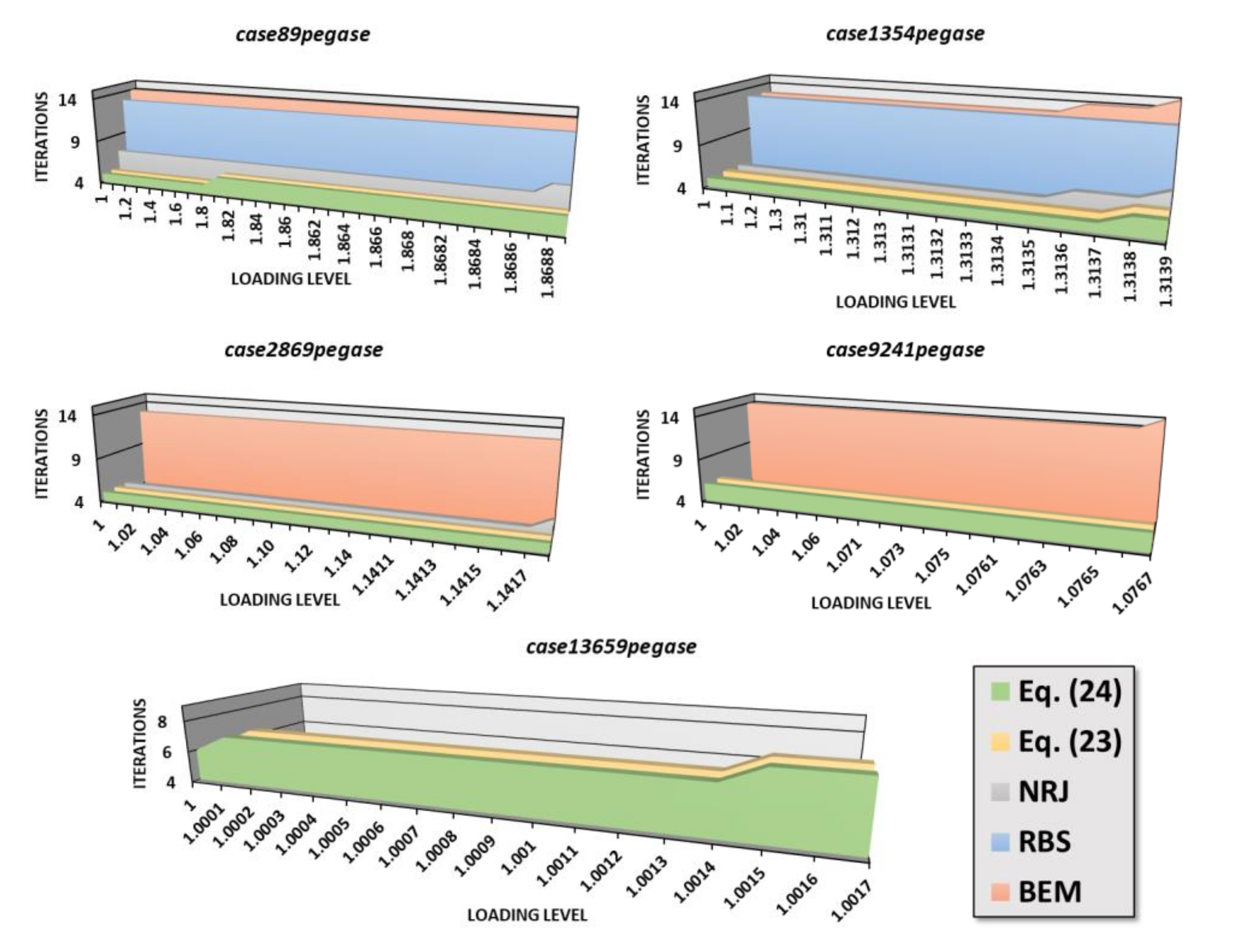
4.5. Influence of the Loading Level

It is well known that the loading level may affect the overall performance of a PF solver. Typically, PF solvers require more iterations as the loading level grows. In some cases, this factor may even provoke instability. Figure 2 shows the total iterations of the studied solvers for different loading levels without reactive limits. The loading levels for the studied cases have been modified by multiplying the injected active and reactive power at PQ buses along with the injected reactive power at PV buses by a real positive factor (called loading level). As observed, our solvers and NRJ normally required less iterations than BEM and RBS. Nevertheless, it is worth noting that the developed techniques required fewer iterations than NRJ for high loading levels. To provide a clearer interpretation of the Figure 2,

Table 9. Total number of iterations at the maximum loadability point.

Method	89-Bus	1354-Bus	2869-Bus	9241-Bus	13659-Bus
RBS	13	13	--	--	--
BEM	14	15	13	15	--
NRJ	8	7	6	--	--
Equation (23)	6	6	5	6	8
Equation (24)	6	6	5	6	8

reports the total iterations required by the different solvers only at the maximum loadability point.

5. Conclusions and Future Works

Inspired by the similitude observed between the methodology described in [6] and the Explicit Midpoint method, we have developed a novel framework for developing efficient and robust PF solution approaches based on Runge–Kutta formulas. This solution paradigm allows adapting any member of the Runge–Kutta family to the PF problem. Although this idea is similar to that described by Milano in [1], the developed framework presents two important advantages:

• The influence of the step size vanishes from the formulation, which means that the developed solution paradigm is intrinsically robust.
• High convergence rates can be achieved, even higher than two.

Explicit and Embedded formulations of the developed solution paradigm have been discussed, and two PF solution techniques based on the Explicit Heun and Embedded Heun–Euler’s methods with cubic order of convergence have been developed.

The developed techniques have been validated using the EU PEGASE systems considering different demanding scenarios. Results have been compared with those obtained with other well-known robust and conventional PF solutions approaches. Our proposals turned out to be more stable and efficient than the other tested techniques, which occasionally showed an unstable behaviour or a high computational cost.

On the basis of the results obtained, it is concluded that the introduced solution paradigm constitutes a promising framework for developing novel PF solution techniques. This opens the door for further applying the developed solution paradigms. Future works should be focused on developing and validating other PF solution techniques, applying other members of the Runge–Kutta family to the developed solution framework. Similarly, analogies between the introduced solution paradigm and other families of numerical integration techniques such as Adams–Bashforth’s methods [8] or Bulirsch–Stoer’s scheme [9] can be found and, consequently, other high-order robust PF solution approaches can be developed. We expect the emergence of this kind of techniques.

The developed solution techniques may be also adapted to other Power System tools such as the Continuation Power-Flow [26]. Here, their robustness along its high convergence order may bring very good results. Future works should study the application of the introduced PF solution techniques to this problem.

References

1. Milano, F. Continuous Newton’s Method for Power Flow Analysis. IEEE Trans. Power Syst. 2009, 24, 50–57. [Google Scholar] [CrossRef]
2. Xie, N.; Torelli, F.; Bompard, E.; Vaccaro, A. Dynamic computing paradigm for comprehensive power flow analysis. IET Gener. Transmiss. Distrib. 2013, 7, 832–842. [Google Scholar] [CrossRef]
3. Iwamoto, S.; Tamura, Y. A load flow calculation method for ill-conditioned power systems. IEEE Trans. Power Appar. Syst. 1981, PAS-100, 1736–1743. [Google Scholar] [CrossRef]
4. Milano, F. Power System Modelling and Scripting; Springer: New York, NY, USA, 2010. [Google Scholar]
5. Braz, L.M.C.; Castro, C.A.; Murati, C.A.F. A critical evaluation of step size optimization based load flow methods. IEEE Trans. Power Syst. 2000, 15, 202–207. [Google Scholar] [CrossRef]
6. Lagace, P.J. Power flow methods for improving convergence. In Proceedings of the IECON 2012—38th Annual Conference on IEEE Industrial Electronics Society, Montreal, QC, USA, 25–28 October 2012; pp. 1387–1392. [Google Scholar] [CrossRef]
7. Tostado-Véliz, M.; Kamel, S.; Jurado, F. Development of combined Runge–Kutta Broyden’s load flow approach for well- and ill-conditioned power systems. IET Gener. Transmiss. Distrib. 2018, 12, 5723–5729. [Google Scholar] [CrossRef]
8. Tostado-Véliz, M.; Kamel, S.; Jurado, F. Development of different load flow methods for solving large-scale ill-conditioned systems. Int. Trans. Elect. Energy Syst. 2019, 29, e2784. [Google Scholar] [CrossRef]
9. Tostado-Véliz, M.; Kamel, S.; Jurado, F. A Robust Power Flow Algorithm Based on Bulirsch-Stoer Method. IEEE Trans. Power Syst. 2019, 34, 3081–3089. [Google Scholar] [CrossRef]
10. Tostado-Véliz, M.; Kamel, S.; Jurado, F. Comparison of various robust and efficient load-flow techniques based on Runge-Kutta formulas. Elect. Power Syst. Res. 2019, 174, 105881. [Google Scholar] [CrossRef]
11. Tostado-Véliz, M.; Kamel, S.; Jurado, F. A powerful power-flow method based on Composite Newton-Cotes formula for ill-conditioned power systems. Int. J. Elect. Power Energy Syst. 2020, 116, 105558. [Google Scholar] [CrossRef]
12. Milano, F. Implicit Continuous Newton Method for Power Flow Analysis. IEEE Trans. Power Syst. 2019, 34, 3309–3311. [Google Scholar] [CrossRef]
13. Xie, N.; Bompard, E.; Napoli, R.; Torelli, F. Widely convergent method for finding solutions of simultaneous nonlinear equations. Elect. Power Syst. Res. 2012, 83, 9–18. [Google Scholar] [CrossRef]
14. Milano, F. Analogy and Convergence of Levenberg’s and Lyapunov-Based Methods for Power Flow Analysis. IEEE Trans. Power Syst. 2016, 31, 1663–1664. [Google Scholar] [CrossRef]
15. Pourbagher, R.; Derakhshandeh, S.Y. Application of high-order Levenberg-Marquardt method for solving the power flow problem in the ill-conditioned systems. IET Gener. Transmiss. Distrib. 2016, 10, 3017–3022. [Google Scholar] [CrossRef]
16. Tostado, M.; Kamel, S.; Jurado, F. An effective load-flow approach based on Gauss-Newton formulation. Int. J. Elect. Power Energy Syst. 2019, 113, 573–581. [Google Scholar] [CrossRef]
17. Rao, S.; Feng, Y.; Tylavsky, D.J.; Subramanian, M.K. The Holomorphic Embedding Method Applied to the Power-Flow Problem. IEEE Trans. Power Syst. 2016, 31, 3816–3828. [Google Scholar] [CrossRef]
18. Tostado, M.; Kamel, S.; Jurado, F. Several robust and efficient load flow techniques based on combined approach for ill-conditioned power systems. Int. J. Elect. Power Energy Syst. 2019, 110, 349–356. [Google Scholar] [CrossRef]
19. Butcher, J.C. Numerical Methods for Ordinary Differential Equations; Wiley: Hoboken, NJ, USA, 2003. [Google Scholar]
20. Tostado-Véliz, M.; Kamel, S.; Jurado, F. Promising Framework Based on Multistep Continuous Newton Scheme for Developing Robust PF Methods. IET Gener. Transmiss. Distrib. 2020, 14, 265–274. [Google Scholar] [CrossRef]
21. Tostado-Véliz, M.; Kamel, S.; Jurado, F. Robust and efficient approach based on Richardson extrapolation for solving badly initialised/ill-conditioned power-flow problems. IET Gener. Transmiss. Distrib. 2019, 13, 3524–3533. [Google Scholar] [CrossRef]
22. Zimmerman, R.D.; Murillo-Sánchez, C.E.; Thomas, R.J. Matpower: Steady-State Operations, Planning and Analysis Tools for Power Systems Research and Education. IEEE Trans. Power Syst. 2011, 26, 12–19. [Google Scholar] [CrossRef] [Green Version]
23. Josz, C.; Fliscounakis, S.; Maeght, J.; Panciatici, P. AC power flow data in MATPOWER and QCQP format: ITesla, RTE snapshots, and PEGASE. arXiv 2016, arXiv:1603.01533. Available online: http://arxiv.org/abs/1603.01533 (accessed on 1 June 2021).
24. Fliscounakis, S.; Panciatici, P.; Capitanescu, F.; Wehenkel, L. Contingency Ranking With Respect to Overloads in Very Large Power Systems Taking Into Account Uncertainty, Preventive, and Corrective Actions. IEEE Trans. Power Syst. 2013, 28, 4909–4917. [Google Scholar] [CrossRef] [Green Version]
25. Modified Matpower EU PEGASE Systems. Available online: https://zenodo.org/record/3553615 (accessed on 1 June 2021). [CrossRef]
26. Ajjarapu, V.; Christy, C. The continuation power flow: A tool for steady state voltage stability analysis. IEEE Trans. Power Syst. 1992, 7, 416–423. [Google Scholar] [CrossRef]
27. Cordero, A.; Villalba, E.G.; Torregrosa, J.R.; Triguero-Navarro, P. Convergence and Stability of a Parametric Class of Iterative Schemes for Solving Nonlinear Systems. Mathematics 2021, 9, 86. [Google Scholar] [CrossRef]
Figure 1. Flowchart of the considered strategy for handling with reactive limits in generation units.
Applsci 11 06147 g001
Figure 2. Total number of iterations for high loading levels.
Applsci 11 06147 g002