
Determining Optimal Power Flow Solutions Using New Adaptive Gaussian TLBO Method


Abstract
:1. Introduction
- A new adaptive Gaussian mutation is integrated into the conventional TLBOs to enhance its exploration and exploration capabilities.
- The proposed algorithm can resolve a wide range of OPF problems for IEEE 30-bus, 57-bus, and 118-bus standard power systems with better outcomes than the state-of-the-art metaheuristic algorithms.
- Many-objective OPF problems to reduce the loss, emission, fuel cost, and voltage deviation in 12 cases are considered and solved by the proposed method to confirm its performance and applicability for various kinds of OPF problems.
2. OPF Problem Formulation
2.1. Problem Constraints
2.1.1. Equality Constraints
2.1.2. Inequality Constraints of the OPF Problem
- Constraints relating to the generation units
- According to [14], the transformers’ taps can be adjusted as follows.where and present the upper and lower values for ith.
- As stated in [14], the generation of volt ampere reactive (VAR) compensating units are constrained as follows.where and are the allowable range of VAR injection of ith compensating unit and NC is the number of the VAR compensating units in the network. The highest apparent power transfer across branches and the acceptable range of load bus voltage magnitudes are known as security constraints [14]:
2.2. Constraint Handling
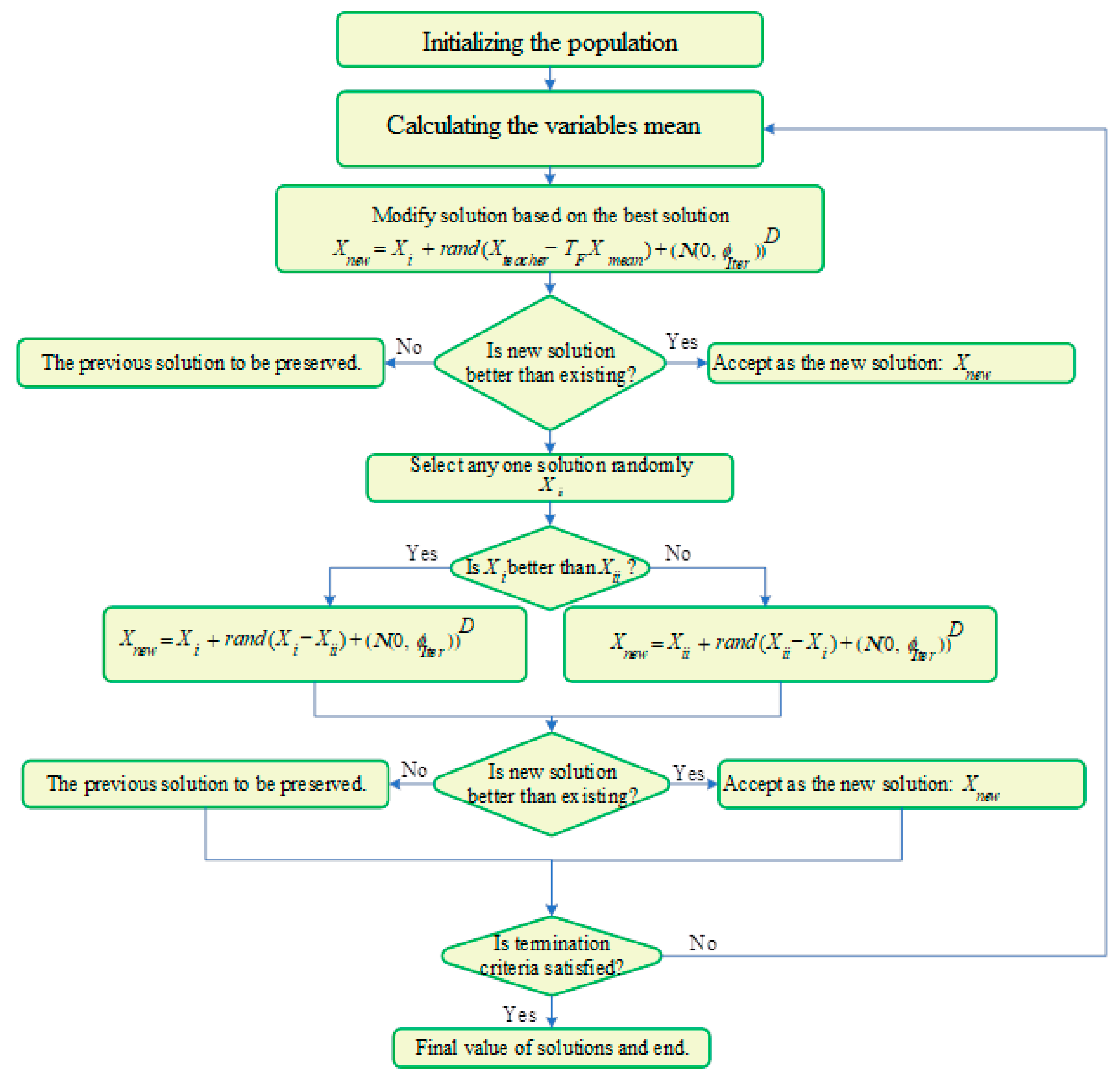
3. Proposed Algorithm
3.1. TLBO
3.1.1. Teaching Phase
3.1.2. Learning Phase
3.2. GTLBO Using Gaussian Mutation Strategy
3.2.1. Gaussian Distribution
3.2.2. Adaptive GTLBO
3.3. Solution Method
- Step 1: Initialize AGTLBO using the parameters from the under-study test system. The maximum number of iterations and population (Npop) for the 30-bus system have been chosen 500 and 25, respectively, 1000 and 40 for the 57-bus system, and 5000 and 60 for the 118-bus system.
- Step 2: Using Equations (21)–(24), generate the starting population or students depending on the number of populations for i = 1: Npop, the lowest and maximum values of control variables and , system constraints, and OPF constraint constraints using Equations (4)–(10).
- Step 3: Using the system and OPF problem constraints, determine the under-study objective function of the initially generated solutions based on (11) and (12) and save them as initial answers of the initial population.
- Step 4 (Adaptive Gaussian Teaching phase): Enhance the answers from the previous step based on (21), apply the system and OPF problem constraints, and calculate their under-study objective function based on (11) and (12). Then, during the subsequent iteration, choose the best answer (new student) from the current and prior solutions provided.
- Step 5: Compare the best student solution (new student) to the previous step’s greatest global solution (teacher). If the new student solution is superior to the best global (teacher) solution, the former takes precedence; otherwise, the old (teacher) solution is retained in the algorithm memory.
- Step 6 (Adaptive Gaussian Learning phase): Based on (24) and the system and optimal OPF problem constraints, enhance the previous step solutions and construct their under-study objective function based on (11) and (12). Then, during the subsequent iteration, choose the student’s answer from among the current and previously generated solutions.
- Step 7: Compare the student solution to the previous step’s teacher solution. If the student solution is superior to the teacher solution, the student solution takes precedence over the teacher solution; otherwise, the prior student solution is stored in the algorithm memory.
- Step 8: Has the algorithm termination requirement been met? Proceed to Step 4 and continue the optimization process if yes; if not, proceed to Step 3.
4. Numerical Results
4.1. Cases Definition
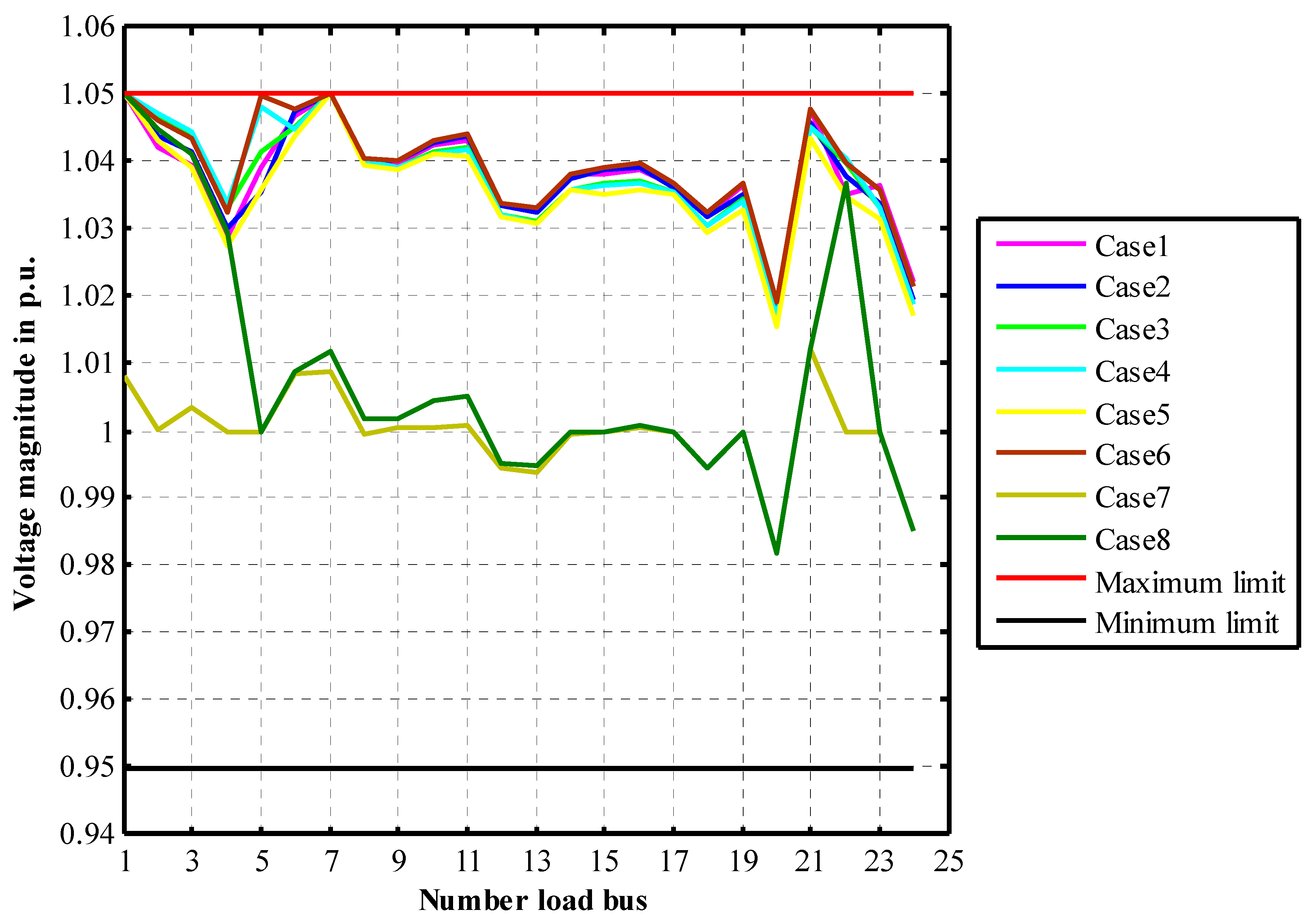
4.1.1. The Studied Cases for the IEEE 30-Bus System
- Minimizing the fuel cost (Case 1).
- Minimizing piecewise quadratic fuel cost functions (Case 2).
- Minimizing the emission (Case 3).
- Minimizing the actual power loss (Case 4).
- Minimizing the fuel cost considering valve point effect (VPE) (Case 5).
- Minimizing the fuel cost and actual power loss (Case 6).
- Minimizing the fuel cost and voltage deviation (Case 7).
- Minimizing the fuel cost, emissions, voltage deviation and losses (Case 8).
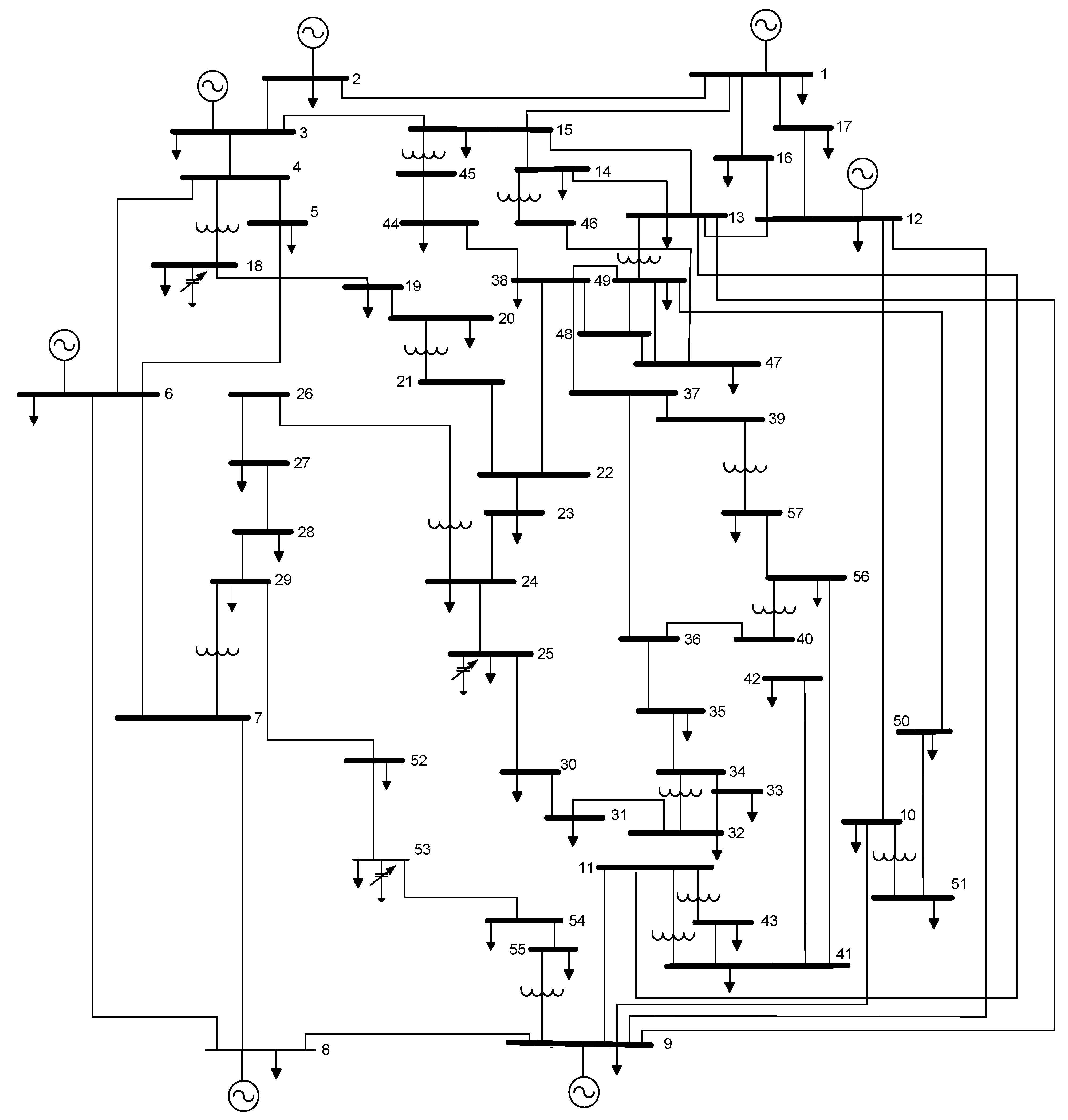
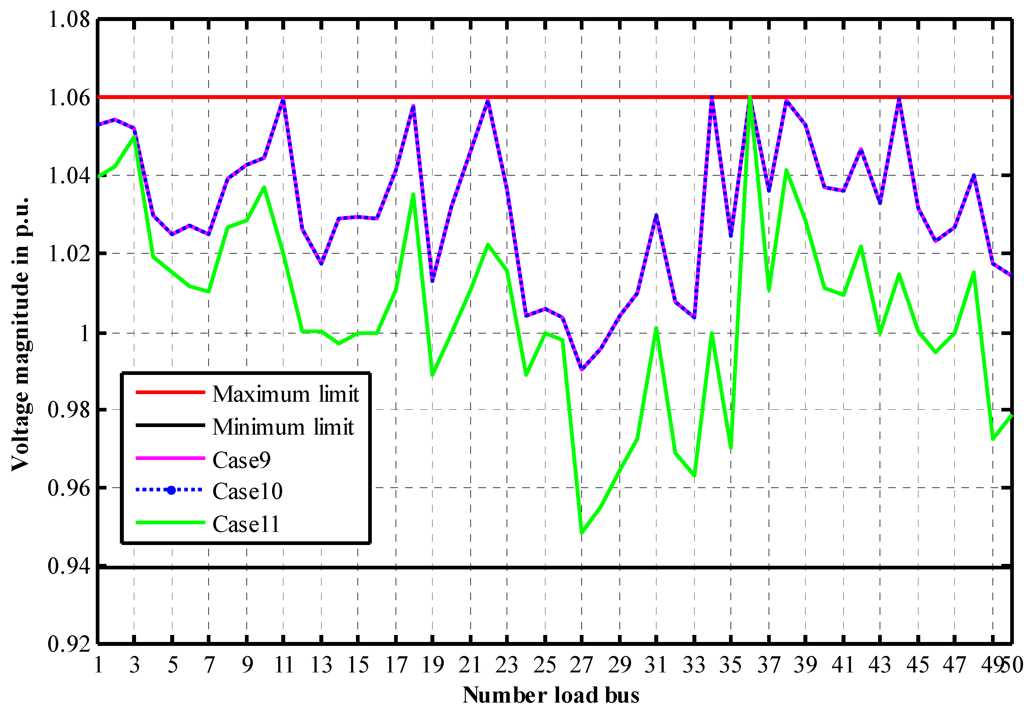
4.1.2. The Studied Cases for the IEEE 57-Bus System
- Minimizing the fuel cost (Case 9).
- Minimizing the fuel cost while improving voltage profile (Case 10).
- Minimizing the fuel cost, emissions, voltage deviation and losses (Case 11).
4.1.3. The Studied Case for the IEEE 118-Bus System
- Minimizing the fuel cost (Case 12).
4.2. EEE 30-Bus Test System
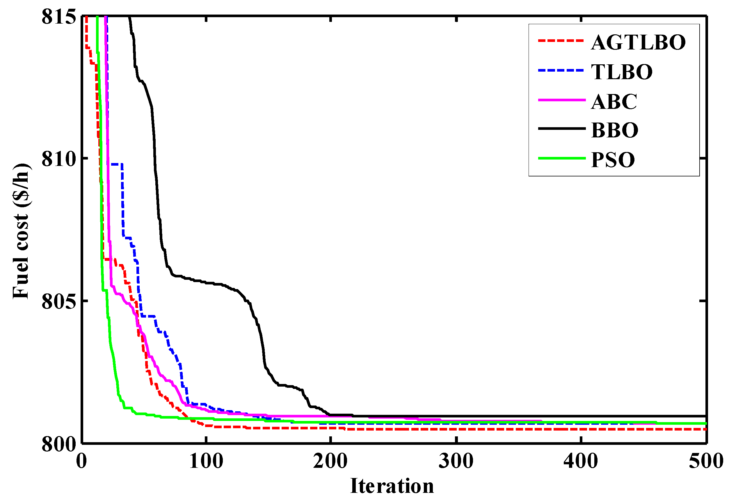
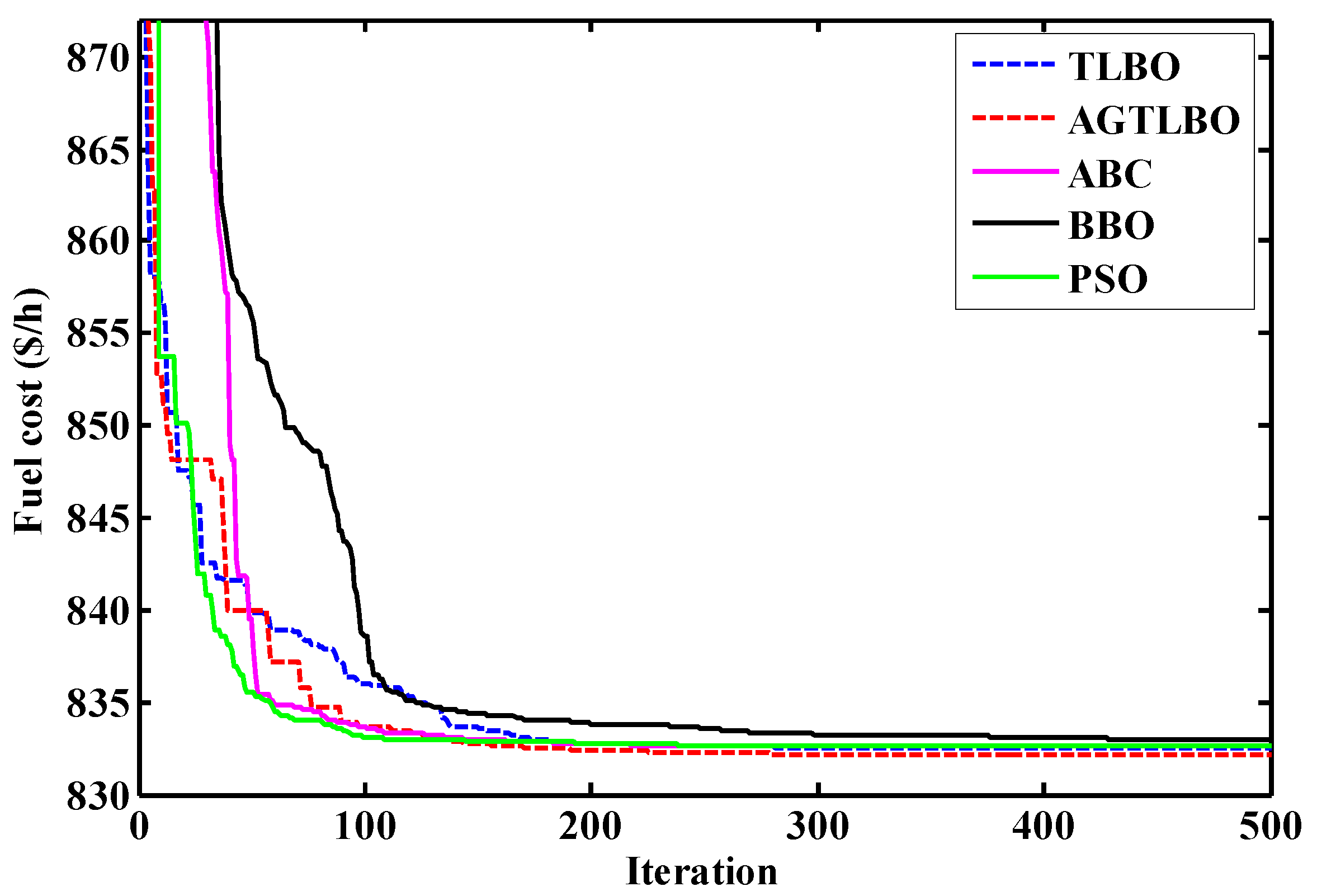
4.2.1. Case 1: Minimizing the Fuel Cost
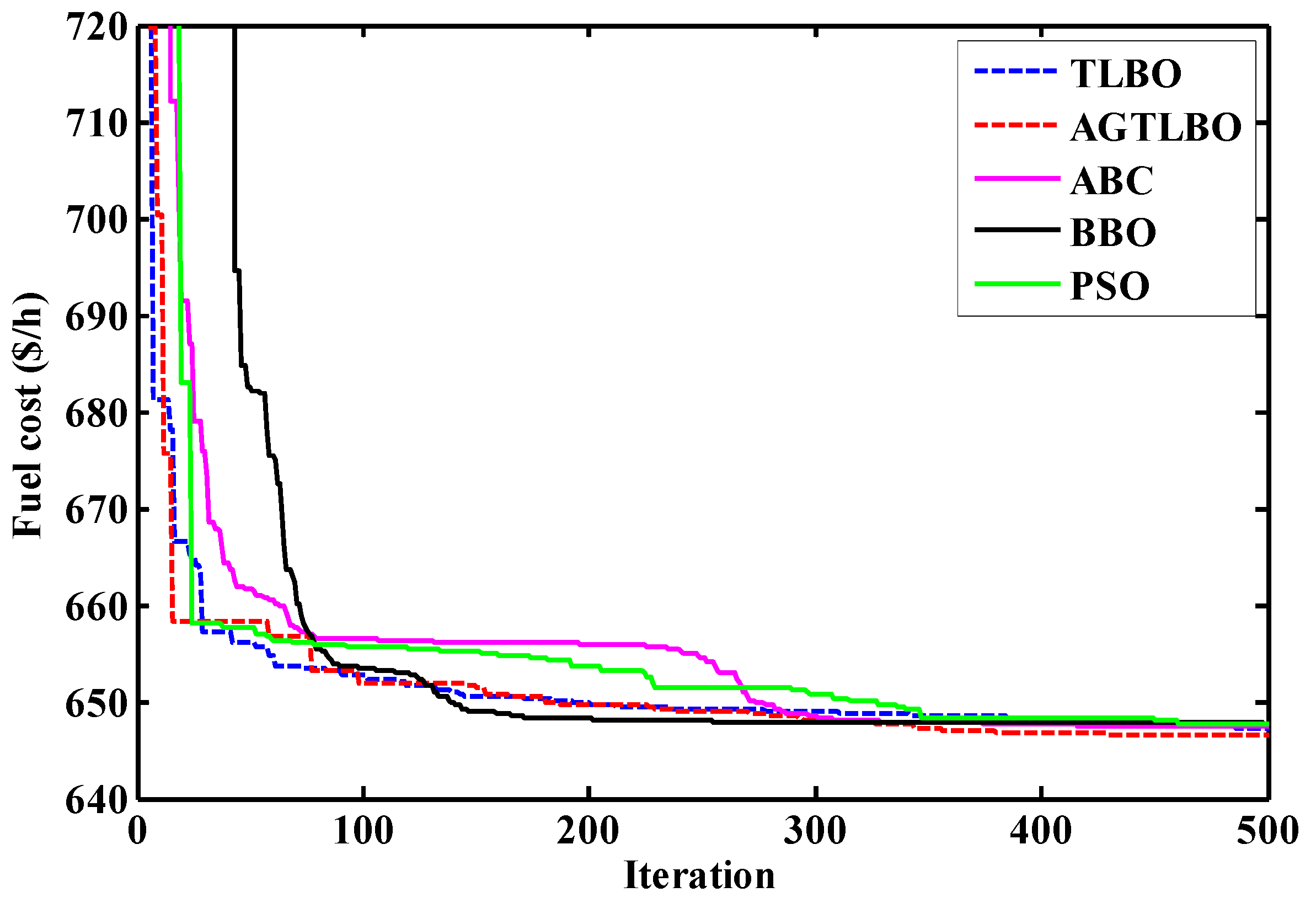
4.2.2. Case 2: Minimizing the Total Fuel Cost Considering Multi-Fuel Sources
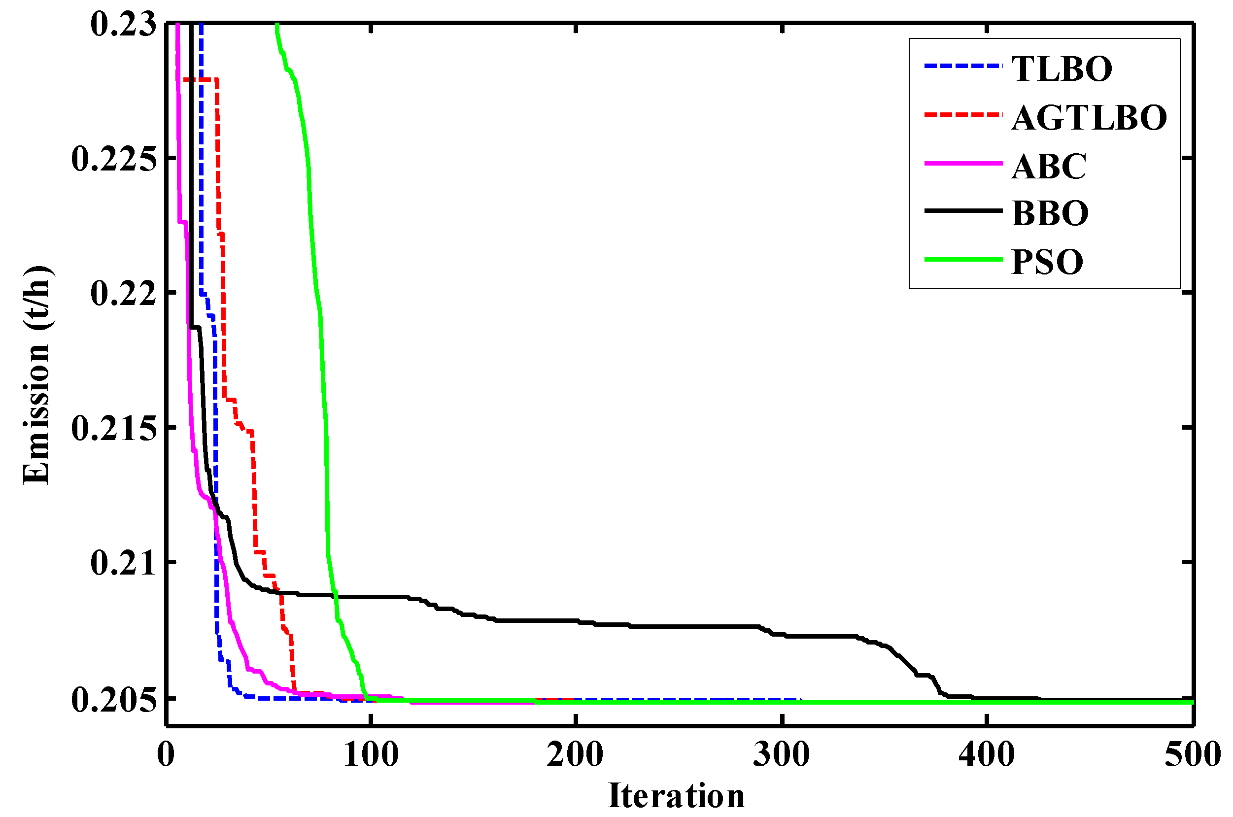
4.2.3. Case 3: Minimizing the Emission
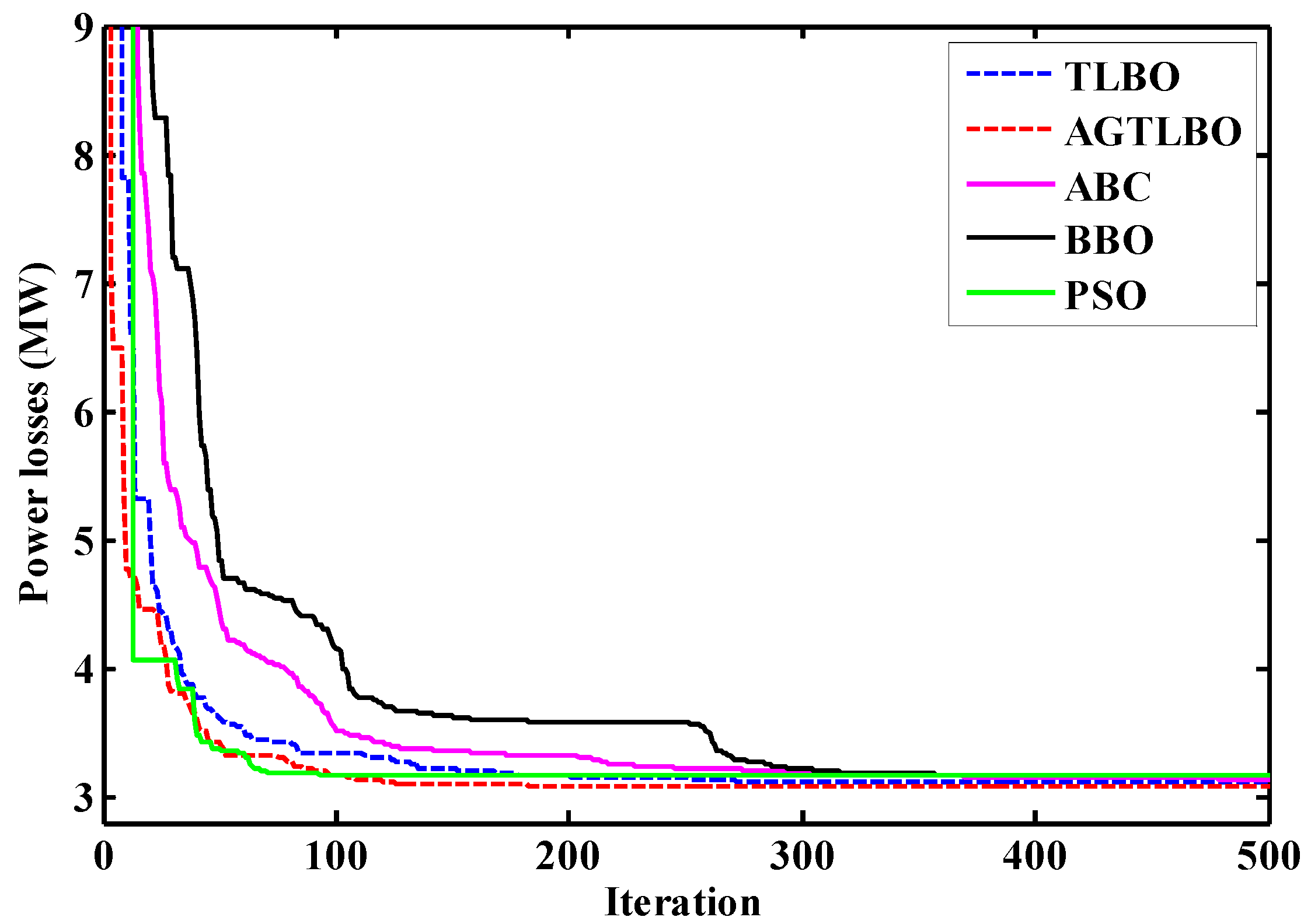
4.2.4. Case 4: Minimizing the Real Power Loss
4.2.5. Case 5: Minimizing the Fuel Cost Considering Valve-Point Effects (VPE)
4.2.6. Case 6: Minimizing the Fuel Cost and Real Power Loss
4.2.7. Case 7: Minimizing the Fuel Cost and Voltage Deviation
4.2.8. Case 8: Minimizing the Fuel Cost, Emission, Voltage Deviation and Losses
4.3. IEEE 57-Bus Test System
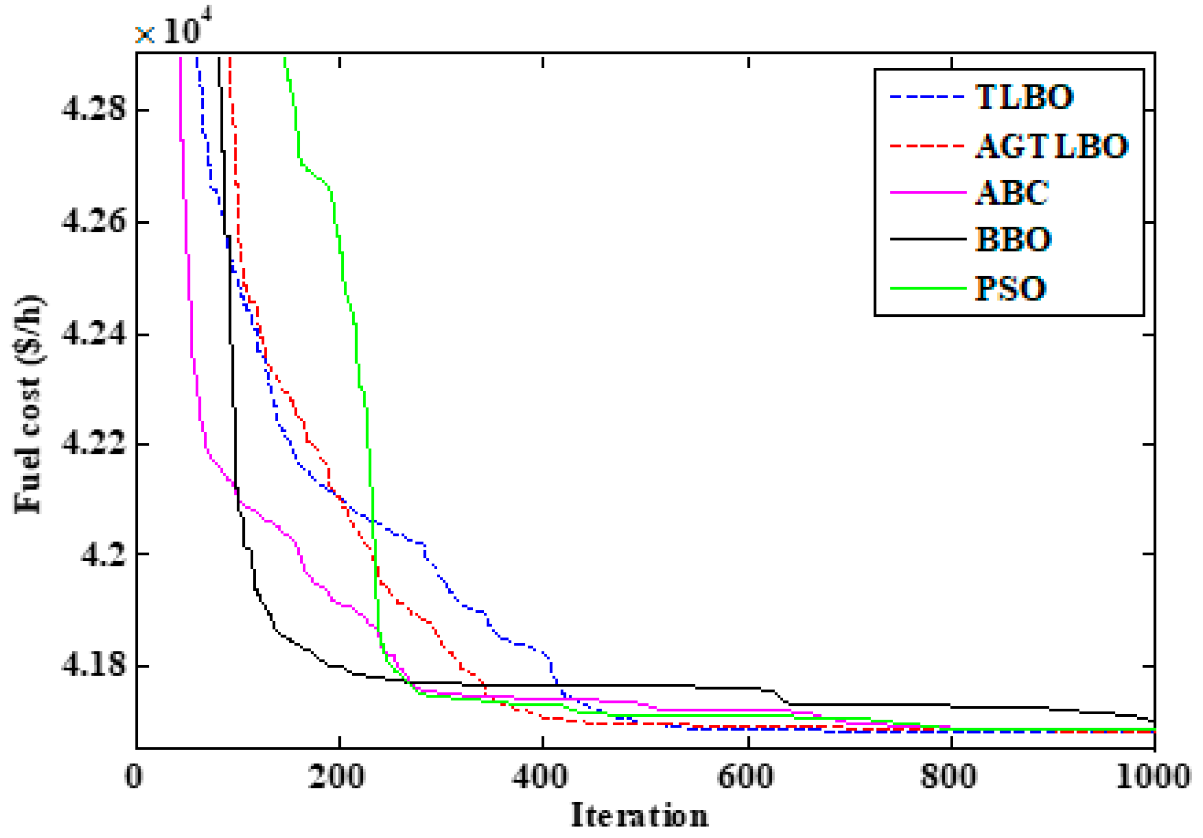
4.3.1. Case 9: Minimizing the Fuel Cost
4.3.2. Case 10: Minimizing the Fuel Cost While Improving Voltage Profile
4.3.3. Case 11: Minimizing the Fuel Cost, Emission, Voltage Deviation and Losses
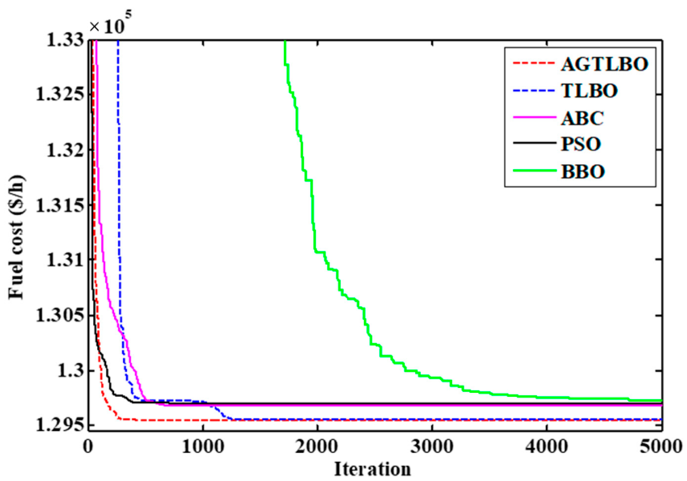
4.4. Case 12: IEEE 118-Bus System
4.5. Discussion on Results
5. Conclusions
Author Contributions
Funding
Institutional Review Board Statement
Informed Consent Statement
Data Availability Statement
Conflicts of Interest
References
- Roy, P.K.; Ghoshal, S.P.; Thakur, S.S. Biogeography based optimization for multi-constraint optimal power flow with emission and non-smooth cost function. Expert Syst. Appl. 2010, 37, 8221–8228. [Google Scholar] [CrossRef]
- Ghasemi, M.; Akbari, M.-A.; Jun, C.; Bateni, S.M.; Zare, M.; Zahedi, A.; Pai, H.-T.; Band, S.S.; Moslehpour, M.; Chau, K.-W. Circulatory System Based Optimization (CSBO): An expert multilevel biologically inspired meta-heuristic algorithm. Eng. Appl. Comput. Fluid Mech. 2022, 16, 1483–1525. [Google Scholar] [CrossRef]
- Akbari, M.A.; Zare, M.; Azizipanah-Abarghooee, R.; Mirjalili, S.; Deriche, M. The cheetah optimizer: A nature-inspired metaheuristic algorithm for large-scale optimization problems. Sci. Rep. 2022, 12, 10953. [Google Scholar] [CrossRef] [PubMed]
- Ghasemi, M.; Rahimnejad, A.; Hemmati, R.; Akbari, E.; Gadsden, S.A. Wild Geese Algorithm: A novel algorithm for large scale optimization based on the natural life and death of wild geese. Array 2021, 11, 100074. [Google Scholar] [CrossRef]
- Abido, M.A. Optimal Power Flow Using Tabu Search Algorithm. Electr. Power Compon. Syst. 2002, 30, 469–483. [Google Scholar] [CrossRef] [Green Version]
- Alghamdi, A.S. A New Self-Adaptive Teaching–Learning-Based Optimization with Different Distributions for Optimal Reactive Power Control in Power Networks. Energies 2022, 15, 2759. [Google Scholar] [CrossRef]
- Islam, M.Z.; Wahab, N.I.A.; Veerasamy, V.; Hizam, H.; Mailah, N.F.; Guerrero, J.M.; Mohd Nasir, M.N. A Harris Hawks optimization based single-and multi-objective optimal power flow considering environmental emission. Sustainability 2020, 12, 5248. [Google Scholar] [CrossRef]
- Jumani, T.A.; Mustafa, M.W.; Md Rasid, M.; Hussain Mirjat, N.; Hussain Baloch, M.; Salisu, S. Optimal power flow controller for grid-connected microgrids using grasshopper optimization algorithm. Electronics 2019, 8, 111. [Google Scholar] [CrossRef] [Green Version]
- Basu, M. Multi-objective optimal power flow with FACTS devices. Energy Convers. Manag. 2011, 52, 903–910. [Google Scholar] [CrossRef]
- Akbari, E.; Ghasemi, M.; Gil, M.; Rahimnejad, A.; Andrew Gadsden, S. Optimal Power Flow via Teaching-Learning-Studying-Based Optimization Algorithm. Electr. Power Compon. Syst. 2022, 49, 584–601. [Google Scholar] [CrossRef]
- Bouchekara, H.R.E.H.; Chaib, A.E.; Abido, M.A.; El-Sehiemy, R.A. Optimal power flow using an Improved Colliding Bodies Optimization algorithm. Appl. Soft Comput. 2016, 42, 119–131. [Google Scholar] [CrossRef]
- Rezaei Adaryani, M.; Karami, A. Artificial bee colony algorithm for solving multi-objective optimal power flow problem. Int. J. Electr. Power Energy Syst. 2013, 53, 219–230. [Google Scholar] [CrossRef]
- Ayan, K.; Kılıç, U.; Baraklı, B. Chaotic artificial bee colony algorithm based solution of security and transient stability constrained optimal power flow. Int. J. Electr. Power Energy Syst. 2015, 64, 136–147. [Google Scholar] [CrossRef]
- Daryani, N.; Hagh, M.T.; Teimourzadeh, S. Adaptive group search optimization algorithm for multi-objective optimal power flow problem. Appl. Soft Comput. 2016, 38, 1012–1024. [Google Scholar] [CrossRef]
- Niknam, T.; Narimani, M.R.; Aghaei, J.; Tabatabaei, S.; Nayeripour, M. Modified Honey Bee Mating Optimisation to solve dynamic optimal power flow considering generator constraints. IET Gener. Transm. Distrib. 2011, 5, 989. [Google Scholar] [CrossRef]
- Mohamed, A.-A.A.; Mohamed, Y.S.; El-Gaafary, A.A.M.; Hemeida, A.M. Optimal power flow using moth swarm algorithm. Electr. Power Syst. Res. 2017, 142, 190–206. [Google Scholar] [CrossRef]
- Khorsandi, A.; Hosseinian, S.H.; Ghazanfari, A. Modified artificial bee colony algorithm based on fuzzy multi-objective technique for optimal power flow problem. Electr. Power Syst. Res. 2013, 95, 206–213. [Google Scholar] [CrossRef]
- Pulluri, H.; Naresh, R.; Sharma, V. An enhanced self-adaptive differential evolution based solution methodology for multiobjective optimal power flow. Appl. Soft Comput. 2017, 54, 229–245. [Google Scholar] [CrossRef]
- Li, S.; Chen, H.; Wang, M.; Heidari, A.A.; Mirjalili, S. Slime mould algorithm: A new method for stochastic optimization. Futur. Gener. Comput. Syst. 2020, 111, 300–323. [Google Scholar] [CrossRef]
- Venkateswara Rao, B.; Nagesh Kumar, G.V. Optimal power flow by BAT search algorithm for generation reallocation with unified power flow controller. Int. J. Electr. Power Energy Syst. 2015, 68, 81–88. [Google Scholar] [CrossRef]
- Narimani, M.R.; Azizipanah-Abarghooee, R.; Zoghdar-Moghadam-Shahrekohne, B.; Gholami, K. A novel approach to multi-objective optimal power flow by a new hybrid optimization algorithm considering generator constraints and multi-fuel type. Energy 2013, 49, 119–136. [Google Scholar] [CrossRef]
- Abaci, K.; Yamacli, V. Differential search algorithm for solving multi-objective optimal power flow problem. Int. J. Electr. Power Energy Syst. 2016, 79, 1–10. [Google Scholar] [CrossRef]
- Jeddi, B.; Einaddin, A.H.; Kazemzadeh, R. Optimal power flow problem considering the cost, loss, and emission by multi-objective electromagnetism-like algorithm. In Proceedings of the 6th IEEE Conference on Thermal Power Plants (CTPP), Tehran, Iran, 19–20 January 2016; pp. 38–45. [Google Scholar]
- He, X.; Wang, W.; Jiang, J.; Xu, L. An Improved Artificial Bee Colony Algorithm and Its Application to Multi-Objective Optimal Power Flow. Energies 2015, 8, 2412–2437. [Google Scholar] [CrossRef] [Green Version]
- El-Fergany, A.A.; Hasanien, H.M. Single and Multi-objective Optimal Power Flow Using Grey Wolf Optimizer and Differential Evolution Algorithms. Electr. Power Compon. Syst. 2015, 43, 1548–1559. [Google Scholar] [CrossRef]
- Ghasemi, M.; Ghavidel, S.; Akbari, E.; Vahed, A.A. Solving non-linear, non-smooth and non-convex optimal power flow problems using chaotic invasive weed optimization algorithms based on chaos. Energy 2014, 73, 340–353. [Google Scholar] [CrossRef]
- Attia, A.-F.; El Sehiemy, R.A.; Hasanien, H.M. Optimal power flow solution in power systems using a novel Sine-Cosine algorithm. Int. J. Electr. Power Energy Syst. 2018, 99, 331–343. [Google Scholar] [CrossRef]
- Ghasemi, M.; Ghavidel, S.; Gitizadeh, M.; Akbari, E. An improved teaching–learning-based optimization algorithm using Lévy mutation strategy for non-smooth optimal power flow. Int. J. Electr. Power Energy Syst. 2015, 65, 375–384. [Google Scholar] [CrossRef]
- Yuan, X.; Zhang, B.; Wang, P.; Liang, J.; Yuan, Y.; Huang, Y.; Lei, X. Multi-objective optimal power flow based on improved strength Pareto evolutionary algorithm. Energy 2017, 122, 70–82. [Google Scholar] [CrossRef]
- Herbadji, O.; Slimani, L.; Bouktir, T. Optimal power flow with four conflicting objective functions using multiobjective ant lion algorithm: A case study of the algerian electrical network. Iran. J. Electr. Electron. Eng. 2019, 15, 94–113. [Google Scholar] [CrossRef]
- Chandrasekaran, S. Multiobjective optimal power flow using interior search algorithm: A case study on a real-time electrical network. Comput. Intell. 2020, 36, 1078–1096. [Google Scholar] [CrossRef]
- Warid, W.; Hizam, H.; Mariun, N.; Abdul-Wahab, N. Optimal Power Flow Using the Jaya Algorithm. Energies 2016, 9, 678. [Google Scholar] [CrossRef]
- Elattar, E.E.; ElSayed, S.K. Modified JAYA algorithm for optimal power flow incorporating renewable energy sources considering the cost, emission, power loss and voltage profile improvement. Energy 2019, 178, 598–609. [Google Scholar] [CrossRef]
- Alghamdi, A.S. Optimal Power Flow of Renewable-Integrated Power Systems Using a Gaussian Bare-Bones Levy-Flight Firefly Algorithm. Front. Energy Res. 2022, 10, 921936. [Google Scholar] [CrossRef]
- Li, S.; Gong, W.; Wang, L.; Yan, X.; Hu, C. Optimal power flow by means of improved adaptive differential evolution. Energy 2020, 198, 117314. [Google Scholar] [CrossRef]
- Panda, A.; Tripathy, M.; Barisal, A.K.; Prakash, T. A modified bacteria foraging based optimal power flow framework for Hydro-Thermal-Wind generation system in the presence of STATCOM. Energy 2017, 124, 720–740. [Google Scholar] [CrossRef]
- Nguyen, T.T. A high performance social spider optimization algorithm for optimal power flow solution with single objective optimization. Energy 2019, 171, 218–240. [Google Scholar] [CrossRef]
- Surender Reddy, S.; Srinivasa Rathnam, C. Optimal Power Flow using Glowworm Swarm Optimization. Int. J. Electr. Power Energy Syst. 2016, 80, 128–139. [Google Scholar] [CrossRef]
- Tran, Q.T.T.; Riva Sanseverino, E.; Zizzo, G.; Di Silvestre, M.L.; Nguyen, T.L.; Tran, Q.-T. Real-time minimization power losses by driven primary regulation in islanded microgrids. Energies 2020, 13, 451. [Google Scholar] [CrossRef] [Green Version]
- Ali, M.A.; Kamel, S.; Hassan, M.H.; Ahmed, E.M.; Alanazi, M. Optimal Power Flow Solution of Power Systems with Renewable Energy Sources Using White Sharks Algorithm. Sustainability 2022, 14, 6049. [Google Scholar] [CrossRef]
- Houssein, E.H.; Hassan, M.H.; Mahdy, M.A.; Kamel, S. Development and application of equilibrium optimizer for optimal power flow calculation of power system. Appl. Intell. 2022, 1–22, advance online publication. [Google Scholar] [CrossRef]
- Sarhan, S.; El-Sehiemy, R.; Abaza, A.; Gafar, M. Turbulent Flow of Water-Based Optimization for Solving Multi-Objective Technical and Economic Aspects of Optimal Power Flow Problems. Mathematics 2022, 10, 2106. [Google Scholar] [CrossRef]
- Sarhan, S.; Shaheen, A.M.; El-Sehiemy, R.A.; Gafar, M. Enhanced Teaching Learning-Based Algorithm for Fuel Costs and Losses Minimization in AC-DC Systems. Mathematics 2022, 10, 2337. [Google Scholar] [CrossRef]
- Rao, R.V.; Savsani, V.J.; Vakharia, D.P. Teaching–Learning-Based Optimization: An optimization method for continuous non-linear large scale problems. Inf. Sci. 2012, 183, 1–15. [Google Scholar] [CrossRef]
- Ghasemi, M.; Ghavidel, S.; Rahmani, S.; Roosta, A.; Falah, H. A novel hybrid algorithm of imperialist competitive algorithm and teaching learning algorithm for optimal power flow problem with non-smooth cost functions. Eng. Appl. Artif. Intell. 2014, 29, 54–69. [Google Scholar] [CrossRef]
- Rao, R.V.; Savsani, V.J.; Vakharia, D.P. Teaching–learning-based optimization: A novel method for constrained mechanical design optimization problems. Comput. Des. 2011, 43, 303–315. [Google Scholar] [CrossRef]
- Hinterding, R. Gaussian mutation and self-adaption for numeric genetic algorithms. In Proceedings of the 1995 IEEE International Conference on Evolutionary Computation, Perth, Australia, 29 November–1 December 1995; Volume 1, p. 384. [Google Scholar]
- Niknam, T.; Zare, M.; Aghaei, J.; Farsani, E.A. A new hybrid evolutionary optimization algorithm for distribution feeder reconfiguration. Appl. Artif. Intell. 2011, 25, 951–971. [Google Scholar] [CrossRef]
- Sayah, S.; Zehar, K. Modified differential evolution algorithm for optimal power flow with non-smooth cost functions. Energy Convers. Manag. 2008, 49, 3036–3042. [Google Scholar] [CrossRef]
- Ongsakul, W.; Tantimaporn, T. Optimal Power Flow by Improved Evolutionary Programming. Electr. Power Compon. Syst. 2006, 34, 79–95. [Google Scholar] [CrossRef]
- Ramesh Kumar, A.; Premalatha, L. Optimal power flow for a deregulated power system using adaptive real coded biogeography-based optimization. Int. J. Electr. Power Energy Syst. 2015, 73, 393–399. [Google Scholar] [CrossRef]
- Pulluri, H.; Naresh, R.; Sharma, V. A solution network based on stud krill herd algorithm for optimal power flow problems. Soft Comput. 2018, 22, 159–176. [Google Scholar] [CrossRef]
- Niknam, T.; Narimani, M.R.; Jabbari, M.; Malekpour, A.R. A modified shuffle frog leaping algorithm for multi-objective optimal power flow. Energy 2011, 36, 6420–6432. [Google Scholar] [CrossRef]
- Ghasemi, M.; Ghavidel, S.; Ghanbarian, M.M.; Gitizadeh, M. Multi-objective optimal electric power planning in the power system using Gaussian bare-bones imperialist competitive algorithm. Inf. Sci. 2015, 294, 286–304. [Google Scholar] [CrossRef]
- Radosavljević, J.; Klimenta, D.; Jevtić, M.; Arsić, N. Optimal Power Flow Using a Hybrid Optimization Algorithm of Particle Swarm Optimization and Gravitational Search Algorithm. Electr. Power Compon. Syst. 2015, 43, 1958–1970. [Google Scholar] [CrossRef]
- SOOD, Y. Evolutionary programming based optimal power flow and its validation for deregulated power system analysis. Int. J. Electr. Power Energy Syst. 2007, 29, 65–75. [Google Scholar] [CrossRef]
- Roy, R.; Jadhav, H.T. Optimal power flow solution of power system incorporating stochastic wind power using Gbest guided artificial bee colony algorithm. Int. J. Electr. Power Energy Syst. 2015, 64, 562–578. [Google Scholar] [CrossRef]
- Surender Reddy, S.; Bijwe, P.R.; Abhyankar, A.R. Faster evolutionary algorithm based optimal power flow using incremental variables. Int. J. Electr. Power Energy Syst. 2014, 54, 198–210. [Google Scholar] [CrossRef]
- Kumari, M.S.; Maheswarapu, S. Enhanced Genetic Algorithm based computation technique for multi-objective Optimal Power Flow solution. Int. J. Electr. Power Energy Syst. 2010, 32, 736–742. [Google Scholar] [CrossRef]
- Singh, R.P.; Mukherjee, V.; Ghoshal, S.P. Particle swarm optimization with an aging leader and challengers algorithm for the solution of optimal power flow problem. Appl. Soft Comput. 2016, 40, 161–177. [Google Scholar] [CrossRef]
- Biswas, P.P.; Suganthan, P.N.; Mallipeddi, R.; Amaratunga, G.A.J. Optimal power flow solutions using differential evolution algorithm integrated with effective constraint handling techniques. Eng. Appl. Artif. Intell. 2018, 68, 81–100. [Google Scholar] [CrossRef]
- Ghasemi, M.; Ghavidel, S.; Ghanbarian, M.M.; Gharibzadeh, M.; Azizi Vahed, A. Multi-objective optimal power flow considering the cost, emission, voltage deviation and power losses using multi-objective modified imperialist competitive algorithm. Energy 2014, 78, 276–289. [Google Scholar] [CrossRef]
- Vaisakh, K.; Srinivas, L.R. Evolving ant direction differential evolution for OPF with non-smooth cost functions. Eng. Appl. Artif. Intell. 2011, 24, 426–436. [Google Scholar] [CrossRef]
- Duman, S.; Güvenç, U.; Sönmez, Y.; Yörükeren, N. Optimal power flow using gravitational search algorithm. Energy Convers. Manag. 2012, 59, 86–95. [Google Scholar] [CrossRef]
- Meng, A.; Zeng, C.; Wang, P.; Chen, D.; Zhou, T.; Zheng, X.; Yin, H. A high-performance crisscross search based grey wolf optimizer for solving optimal power flow problem. Energy 2021, 225, 120211. [Google Scholar] [CrossRef]
- Bai, W.; Eke, I.; Lee, K.Y. An improved artificial bee colony optimization algorithm based on orthogonal learning for optimal power flow problem. Control Eng. Pract. 2017, 61, 163–172. [Google Scholar] [CrossRef]
- Shaheen, A.M.; El-Sehiemy, R.A.; Elattar, E.E.; Abd-Elrazek, A.S. A modified crow search optimizer for solving non-linear OPF problem with emissions. IEEE Access 2021, 9, 43107–43120. [Google Scholar] [CrossRef]
- Hassan, M.H.; Kamel, S.; Selim, A.; Khurshaid, T.; Domínguez-García, J.L. A modified Rao-2 algorithm for optimal power flow incorporating renewable energy sources. Mathematics 2021, 9, 1532. [Google Scholar] [CrossRef]
- Nadimi-Shahraki, M.H.; Taghian, S.; Mirjalili, S.; Abualigah, L.; Abd Elaziz, M.; Oliva, D. EWOA-OPF: Effective Whale Optimization Algorithm to Solve Optimal Power Flow Problem. Electronics 2021, 10, 2975. [Google Scholar] [CrossRef]
- Karaboga, D.; Basturk, B. A powerful and efficient algorithm for numerical function optimization: Artificial bee colony (ABC) algorithm. J. Glob. Optim. 2007, 39, 459–471. [Google Scholar] [CrossRef]
- Simon, D. Biogeography-based optimization. IEEE Trans. Evol. Comput. 2008, 12, 702–713. [Google Scholar] [CrossRef] [Green Version]
- Zambrano-Bigiarini, M.; Clerc, M.; Rojas, R. Standard particle swarm optimisation 2011 at cec-2013: A baseline for future pso improvements. In Proceedings of the 2013 IEEE Congress on Evolutionary Computation, Cancun, Mexico, 20–23 June 2013; pp. 2337–2344. [Google Scholar]


| Control Variables Settings | Limits | Case 1 | Case 2 | Case 3 | Case 4 | Case 5 | Case 6 | Case 7 | Case 8 | |
|---|---|---|---|---|---|---|---|---|---|---|
| Lower | Upper | |||||||||
| PG1 (MW) 1 | 50 | 250 | 177.1160 | 139.9996 | 64.0640 | 51.4932 | 198.7677 | 102.6327 | 176.3251 | 122.2170 |
| PG2 (MW) | 20 | 80 | 48.7445 | 54.9999 | 67.5593 | 79.9983 | 44.7547 | 55.5362 | 49.0930 | 52.5169 |
| PG5 (MW) | 15 | 50 | 21.3225 | 24.1810 | 50.0000 | 49.9997 | 18.5617 | 38.1125 | 21.5587 | 31.4731 |
| PG8 (MW) | 10 | 35 | 21.2933 | 34.9987 | 35.0000 | 34.9997 | 10.0000 | 35.0000 | 22.1467 | 35.0000 |
| PG11 (MW) | 10 | 30 | 11.9442 | 18.3761 | 30.0000 | 29.9999 | 10.0010 | 30.0000 | 12.1467 | 26.7432 |
| PG13 (MW) | 12 | 40 | 12.0017 | 17.5743 | 40.0000 | 39.9998 | 12.0012 | 26.6486 | 12.0016 | 21.0381 |
| VG1 (p.u.) | 0.95 | 1.1 | 1.0835 | 1.0756 | 1.0628 | 1.0618 | 1.0810 | 1.0697 | 1.0427 | 1.0729 |
| VG2 (p.u.) | 0.95 | 1.1 | 1.0604 | 1.0583 | 1.0562 | 1.0571 | 1.0577 | 1.0575 | 1.0230 | 1.0573 |
| VG5 (p.u.) | 0.95 | 1.1 | 1.0334 | 1.0328 | 1.0375 | 1.0382 | 1.0302 | 1.0357 | 1.0151 | 1.0326 |
| VG8 (p.u.) | 0.95 | 1.1 | 1.0383 | 1.0414 | 1.0439 | 1.0445 | 1.0368 | 1.0437 | 1.0065 | 1.0411 |
| VG11 (p.u.) | 0.95 | 1.1 | 1.0923 | 1.0937 | 1.0806 | 1.0846 | 1.0968 | 1.0982 | 1.0595 | 1.0401 |
| VG13 (p.u.) | 0.95 | 1.1 | 1.0502 | 1.0563 | 1.0542 | 1.0542 | 1.0606 | 1.0576 | 0.9879 | 1.0235 |
| T6–9 (p.u.) | 0.9 | 1.1 | 1.0669 | 1.0886 | 1.0457 | 1.0237 | 1.0810 | 1.0347 | 1.0830 | 1.0999 |
| T6–10 (p.u.) | 0.9 | 1.1 | 0.9242 | 0.9000 | 0.9403 | 0.9734 | 0.9295 | 0.9498 | 0.9000 | 0.9533 |
| T4–12 (p.u.) | 0.9 | 1.1 | 0.9783 | 0.9853 | 0.9985 | 0.9975 | 0.9980 | 0.9911 | 0.9397 | 1.0322 |
| T28–27 (p.u.) | 0.9 | 1.1 | 0.9737 | 0.9776 | 0.9760 | 0.9766 | 0.9770 | 0.9749 | 0.9708 | 1.0050 |
| QC10 (MVAR) | 0.0 | 5.0 | 4.2404 | 3.6102 | 4.3278 | 4.5447 | 5.0000 | 0.7485 | 5.0000 | 3.5672 |
| QC12 (MVAR) | 0.0 | 5.0 | 2.8095 | 0.0895 | 5.0000 | 4.5668 | 4.6104 | 0.3659 | 0.2788 | 0.3126 |
| QC15 (MVAR) | 0.0 | 5.0 | 4.3275 | 4.8197 | 4.6281 | 4.6210 | 3.8474 | 4.4830 | 4.9929 | 3.8845 |
| QC17 (MVAR) | 0.0 | 5.0 | 5.0000 | 5.0000 | 4.9898 | 4.9974 | 4.8606 | 5.0000 | 0.0050 | 4.9997 |
| QC20 (MVAR) | 0.0 | 5.0 | 5.0000 | 4.0709 | 4.1275 | 4.2175 | 4.8219 | 4.2613 | 4.9988 | 4.9991 |
| QC21 (MVAR) | 0.0 | 5.0 | 4.9972 | 4.9595 | 5.0000 | 4.9995 | 4.9761 | 5.0000 | 4.9407 | 5.0000 |
| QC23 (MVAR) | 0.0 | 5.0 | 3.1538 | 2.9699 | 3.2253 | 3.2410 | 3.5700 | 3.2503 | 4.9995 | 4.3039 |
| QC24 (MVAR) | 0.0 | 5.0 | 5.0000 | 5.0000 | 4.9983 | 4.9998 | 4.9973 | 5.0000 | 4.9993 | 5.0000 |
| QC29 (MVAR) | 0.0 | 5.0 | 2.7696 | 2.6055 | 2.5183 | 2.5435 | 2.4718 | 2.5520 | 2.6307 | 2.6200 |
| Cost ($/h) | - | - | 800.4811 | 646.4511 | 944.3385 | 967.6336 | 832.1624 | 858.9928 | 803.7385 | 830.1559 |
| Emission (t/h) | - | - | 0.3662 | 0.2835 | 0.2048 | 0.2073 | 0.4379 | 0.2290 | 0.3639 | 0.2529 |
| Power losses (MW) | - | - | 9.0222 | 6.7296 | 3.2233 | 3.0906 | 10.6863 | 4.5300 | 9.8718 | 5.5823 |
| V.D. (p.u.) | - | - | 0.9109 | 0.9046 | 0.9017 | 0.9086 | 0.8592 | 0.9428 | 0.0947 | 0.2975 |
| Algorithm | Emission (t/h) | Fuel Cost (USD/h) | V.D. (p.u.) | Power Losses (MW) |
|---|---|---|---|---|
| AGTLBO | 0.3662 | 800.481 | 0.9109 | 9.0222 |
| TLBO | 0.3668 | 800.674 | 0.9120 | 9.0198 |
| TS (Tabu Search) [5] | - | 802.290 | - | - |
| ABC (Artificial Bee Colony) [12] | 0.3651 | 800.660 | 0.9209 | 9.0328 |
| AGSO (Adaptive Group Search Optimization) [14] | 0.3703 | 801.750 | - | - |
| MHBMO (Modified Honey Bee Mating Optimization) [15] | - | 801.985 | - | 9.4900 |
| MSA (Moth Swarm Algorithm) [16] | 0.3665 | 800.510 | 0.9036 | 9.0345 |
| FPA (Flower Pollination Algorithm) [16] | 0.3596 | 802.798 | 0.3679 | 9.5406 |
| MFO (Moth-Flame Optimization) [16] | 0.3685 | 800.686 | 0.7577 | 9.1492 |
| MPSO-SFLA (Modified Particle Swarm Optimization and Shuffle Frog Leaping Algorithm) [21] | - | 801.750 | - | 9.5400 |
| GWO (Grey Wolf Optimizer) [25] | - | 801.410 | - | 9.3000 |
| MICA-TLA (Modified Imperialist Competitive Algorithm and Teaching Learning Algorithm) [45] | - | 801.049 | - | 9.1895 |
| DE (Differential Evolution) [49] | - | 802.390 | - | 9.4660 |
| SKH (Stud Krill Herd Algorithm) [52] | 0.3662 | 800.514 | - | 9.0282 |
| SFLA-SA (Shuffle Frog Leaping Algorithm and Simulated Annealing) [53] | - | 801.790 | - | - |
| ARCBBO (Adaptive Real Coded Biogeography-Based Optimization) [51] | 0.3663 | 800.516 | 0.8867 | 9.0255 |
| MGBICA (Modified Gaussian Bare-Bones Imperialist Competitive Algorithm) [54] | 0.3296 | 801.141 | - | - |
| IEP (Improved Evolutionary Programming) [50] | - | 802.460 | - | - |
| PSOGSA (Particle Swarm Optimization and Gravitational Search Algorithm) [55] | - | 800.499 | 0.1267 | 9.0339 |
| EP (Evolutionary Programming) [56] | - | 803.570 | - | - |
| Algorithm | Emission (t/h) | Fuel Cost (USD/h) | V.D. (p.u.) | Power Losses (MW) |
|---|---|---|---|---|
| AGTLBO | 0.2835 | 646.4511 | 0.9046 | 6.7296 |
| TLBO | 0.2835 | 647.1344 | 0.8927 | 6.8409 |
| LTLBO (Lévy Teaching–Learning-Based Optimization) [28] | 0.2835 | 647.4315 | 0.8896 | 6.9347 |
| MDE (Modified Differential Evolution) [49] | - | 647.8460 | - | 7.095 |
| MFO (Moth-Flame Optimization) [16] | 0.28336 | 649.2727 | 0.47024 | 7.2293 |
| IEP (Improved Evolutionary Programming) [50] | - | 649.3120 | - | - |
| MICA-TLA (Modified Imperialist Competitive Algorithm and Teaching Learning Algorithm) [45] | - | 647.1002 | - | 6.8945 |
| FPA (Flower Pollination Algorithm) [16] | 0.28083 | 651.3768 | 0.31259 | 7.2355 |
| SSO (Social Spider Optimization) [37] | - | 663.3518 | - | - |
| GABC (Gbest Guided Artificial Bee Colony Algorithm) [57] | - | 647.0300 | 0.8010 | 6.8160 |
| MSA (Moth Swarm Algorithm) [16] | 0.28352 | 646.8364 | 0.84479 | 6.8001 |
| MPSO-SFLA (Modified Particle Swarm Optimization and Shuffle Frog Leaping Algorithm) [21] | - | 647.5500 | - | - |
| Algorithm | Emission (t/h) | Fuel Cost (USD/h) | V.D. (p.u.) | Power Losses (MW) |
|---|---|---|---|---|
| AGTLBO | 0.2048 | 944.3385 | 0.9017 | 3.2233 |
| TLBO | 0.2048 | 944.5446 | 0.7979 | 3.2944 |
| ARCBBO (Adaptive Real Coded Biogeography-Based Optimization) [51] | 0.2048 | 945.1597 | 0.8647 | 3.2624 |
| ABC (Artificial Bee Colony) [12] | 0.2048 | 944.4391 | 0.8463 | 3.2470 |
| GBICA (Gaussian Bare-Bones Imperialist Competitive Algorithm) [54] | 0.2049 | 944.6516 | - | - |
| FPA (Flower Pollination Algorithm) [16] | 0.2052 | 948.9490 | 0.4276 | 4.4920 |
| AGSO (Adaptive Group Search Optimization) [14] | 0.2059 | 953.6290 | - | - |
| DSA (Differential Search Algorithm) [22] | 0.2058 | 944.4086 | - | 3.2437 |
| MFO (Moth-Flame Optimization) [16] | 0.2049 | 945.4553 | 0.7097 | 3.4295 |
| MSA (Moth Swarm Algorithm) [16] | 0.2048 | 944.5003 | 0.8739 | 3.2358 |
| MSFLA (Modified Shuffle Frog Leaping Algorithm) [53] | 0.2056 | - | - | - |
| MPSO-SFLA (Modified Particle Swarm Optimization and Shuffle Frog Leaping Algorithm) [21] | 0.2052 | - | - | - |
| Algorithm | Emission (t/h) | Fuel Cost (USD/h) | V.D. (p.u.) | Power Losses (MW) |
|---|---|---|---|---|
| AGTLBO | 0.2073 | 967.6336 | 0.9086 | 3.0906 |
| TLBO | 0.2072 | 967.7195 | 0.8821 | 3.1104 |
| ABC (Artificial Bee Colony) [12] | 0.2073 | 967.6810 | 0.9008 | 3.1078 |
| FPA (Flower Pollination Algorithm) [16] | 0.2076 | 967.1138 | 0.3893 | 3.5661 |
| MFO (Moth-Flame Optimization) [16] | 0.2073 | 967.6785 | 0.9156 | 3.1111 |
| MSA (Moth Swarm Algorithm) [16] | 0.2073 | 967.6636 | 0.8887 | 3.1005 |
| DSA (Differential Search Algorithm) [22] | 0.2083 | 967.6493 | - | 3.0945 |
| GWO (Grey Wolf Optimizer) [25] | - | 968.3800 | - | 3.4100 |
| Jaya [32] | - | 967.6827 | 0.1272 | 3.1035 |
| ARCBBO (Adaptive Real Coded Biogeography-Based Optimization) [51] | 0.2073 | 967.6605 | 0.8913 | 3.1009 |
| EEA (Efficient Evolutionary Algorithm) [58] | - | 952.3785 | - | 3.2823 |
| EGA (Enhanced Genetic Algorithm) [58] | - | 967.9300 | - | 3.2440 |
| EGA-DQLF (Enhanced Genetic Algorithm to Decoupled Quadratic Load Flow) [59] | - | 967.8600 | 0.1218 | 3.2008 |
| ALC-PSO (Particle Swarm Optimization with an Aging Leader and Challengers) [60] | - | 967.7683 | - | 3.1700 |
| Algorithm | Emission (t/h) | Fuel Cost (USD/h) | V.D. (p.u.) | Power Losses (MW) |
|---|---|---|---|---|
| AGTLBO | 0.4379 | 832.1624 | 0.8592 | 10.6863 |
| TLBO | 0.4382 | 832.5325 | 0.8654 | 10.6870 |
| PSO (Particle Swarm Optimization) [11] | - | 832.6871 | - | - |
| SP-DE (Differential Evolution Integrated Self-Adaptive Penalty) [61] | 0.43651 | 832.4813 | 0.7504 | 10.6762 |
| Algorithm | Emission (t/h) | Fuel Cost (USD/h) | V.D. (p.u.) | Power Losses (MW) |
|---|---|---|---|---|
| AGTLBO | 0.2290 | 858.9928 | 0.9428 | 4.5300 |
| TLBO | 0.2307 | 859.0191 | 0.9152 | 4.5687 |
| MSA (Moth Swarm Algorithm) [16] | 0.2289 | 859.1915 | 0.92852 | 4.5404 |
| SF-DE (Differential Evolution Integrated Superiority of Feasible Solutions) [61] | 0.2289 | 859.1458 | 0.92731 | 4.5245 |
| Algorithm | Emission (t/h) | Fuel Cost (USD/h) | V.D. (p.u.) | Power Losses (MW) |
|---|---|---|---|---|
| AGTLBO | 0.3639 | 803.7385 | 0.0947 | 9.8718 |
| TLBO | 0.3565 | 804.2391 | 0.1056 | 9.9565 |
| MPSO (Modified Particle Swarm Optimization) [16] | 0.3636 | 803.9787 | 0.1202 | 9.9242 |
| MFO (Moth-Flame Optimization) [16] | 0.36355 | 803.7911 | 0.10563 | 9.8685 |
| MOICA (Multi-Objective Imperialist Competitive Algorithm) [62] | - | 805.0345 | 0.1004 | - |
| NKEA (Neighborhood Knowledge-based Evolutionary Algorithm) [62] | - | 804.9612 | 0.099 | - |
| BB-MOPSO (Bare-Bones Modified Particle Swarm Optimization) [62] | - | 804.9639 | 0.1021 | - |
| MNSGA-II (Modified Non-dominated Sorting GA-II) [62] | - | 805.0076 | 0.0989 | - |
| MOMICA (Multi-Objective Modified Imperialist Competitive Algorithm) [62] | 0.3552 | 804.9611 | 0.0952 | 9.8212 |
| Algorithm | Emission (t/h) | Fuel Cost (USD/h) | V.D. (p.u.) | Power Losses (MW) |
|---|---|---|---|---|
| AGTLBO | 0.2529 | 830.1559 | 0.2975 | 5.5823 |
| TLBO | 0.2538 | 831.3186 | 0.2982 | 5.5847 |
| MFO (Moth-Flame Optimization) [16] | 0.25231 | 830.9135 | 0.33164 | 5.5971 |
| MSA (Moth Swarm Algorithm) [16] | 0.25258 | 830.639 | 0.29385 | 5.6219 |
| MOICA (Multi-Objective Imperialist Competitive Algorithm) [62] | 0.267 | 831.2251 | 0.4046 | 6.0223 |
| NKEA (Neighborhood Knowledge-based Evolutionary Algorithm) [62] | 0.2491 | 834.6433 | 0.4448 | 5.8935 |
| BB-MOPSO (Bare-Bones Modified Particle Swarm Optimization) [62] | 0.2479 | 833.0345 | 0.3945 | 5.6504 |
| MNSGA-II (Modified Non-dominated Sorting GA-II) [62] | 0.2527 | 834.5616 | 0.4308 | 5.6606 |
| MOMICA (Multi-Objective Modified Imperialist Competitive Algorithm) [62] | 0.2523 | 830.1884 | 0.2978 | 5.5851 |
| Control Variables Settings | Algorithms | |||||
|---|---|---|---|---|---|---|
| EADDE (Evolving Ant Direction Differential Evolution) [63] | GSA (Gravitational Search Algorithm) [64] | ABC (Artificial Bee Colony) [12] | MICA (Modified Imperialist Competitive Algorithm) [45] | LTLBO (Lévy Teaching–Learning-Based Optimization) [28] | AGTLBO | |
| PG1 (MW) | 143.150 | 142.369 | 142.811 | 142.520 | 142.870 | 143.910 |
| PG2 (MW) | 95.290 | 92.630 | 90.033 | 88.001 | 88.953 | 92.021 |
| PG3 (MW) | 45.320 | 45.318 | 44.515 | 44.596 | 44.788 | 45.324 |
| PG6(MW) | 73.600 | 72.355 | 74.200 | 72.086 | 72.577 | 70.000 |
| PG8 (MW) | 464.850 | 464.743 | 454.848 | 460.325 | 460.906 | 458.585 |
| PG9 (MW) | 83.440 | 84.999 | 96.885 | 98.354 | 94.179 | 96.025 |
| PG12 (MW) | 361.240 | 363.951 | 362.772 | 360.179 | 361.687 | 360.000 |
| VG1 (p.u.) | 1.050 | 1.059 | 1.042 | 1.033 | 1.038 | 1.060 |
| VG2(p.u.) | 1.048 | 1.058 | 1.041 | 1.037 | 1.042 | 1.059 |
| VG3 (p.u.) | 1.041 | 1.060 | 1.039 | 1.028 | 1.031 | 1.055 |
| VG6 (p.u.) | 1.049 | 1.060 | 1.055 | 1.044 | 1.047 | 1.060 |
| VG8 (p.u.) | 1.056 | 1.060 | 1.064 | 1.060 | 1.060 | 1.060 |
| VG9 (p.u.) | 1.034 | 1.060 | 1.037 | 1.027 | 1.028 | 1.039 |
| VG12 (p.u.) | 1.041 | 1.046 | 1.041 | 1.019 | 1.022 | 1.044 |
| T4–18 (p.u.) | 1.051 | 0.900 | 0.938 | 0.961 | 0.901 | 1.012 |
| T4–18 (p.u.) | 0.907 | 0.900 | 1.050 | 1.004 | 1.080 | 0.966 |
| T21–20 (p.u.) | 1.038 | 0.909 | 0.975 | 1.021 | 1.019 | 1.011 |
| T24–25 (p.u.) | 1.004 | 1.059 | 0.950 | 1.038 | 1.034 | 1.100 |
| T24–25 (p.u.) | 0.962 | 0.999 | 1.013 | 0.972 | 1.025 | 0.970 |
| T24–26 (p.u.) | 0.986 | 0.922 | 1.000 | 1.029 | 1.026 | 1.026 |
| T7–29 (p.u.) | 0.984 | 0.932 | 1.013 | 0.983 | 0.984 | 0.990 |
| T34–32 (p.u.) | 0.908 | 1.088 | 0.913 | 0.963 | 0.971 | 0.964 |
| T11–41 (p.u.) | 0.923 | 1.039 | 0.900 | 0.933 | 0.900 | 0.906 |
| T15–45 (p.u.) | 0.991 | 1.043 | 1.013 | 0.951 | 0.954 | 0.976 |
| T14–46 (p.u.) | 0.982 | 1.025 | 0.988 | 0.935 | 0.940 | 0.966 |
| T10–51 (p.u.) | 0.989 | 0.954 | 1.000 | 0.949 | 0.950 | 0.967 |
| T13–49 (p.u.) | 0.966 | 0.929 | 0.963 | 0.904 | 0.912 | 0.933 |
| T11–43 (p.u.) | 0.972 | 1.099 | 0.963 | 0.941 | 0.948 | 0.965 |
| T40–56 (p.u.) | 0.997 | 0.969 | 0.963 | 1.017 | 0.993 | 0.990 |
| T39–57 (p.u.) | 1.002 | 1.062 | 0.925 | 0.985 | 0.970 | 0.947 |
| T9–55 (p.u.) | 1.045 | 1.094 | 0.988 | 0.974 | 0.972 | 0.996 |
| QC18 (MVAR) | 9.030 | 15.243 | 16.000 | 18.660 | 17.590 | 8.950 |
| QC25 (MVAR) | 8.170 | 14.403 | 15.000 | 13.620 | 17.410 | 18.110 |
| QC53 (MVAR) | 20.130 | 15.102 | 14.000 | 14.310 | 15.080 | 15.410 |
| Cost ($/h) | 41,713.620 | 41,695.872 | 41,693.959 | 41,683.048 | 41,679.545 | 41,678.310 |
| Emission (t/h) | - | - | - | - | - | 1.901 |
| V.D. (p.u.) | 1.098 | - | - | 1.449 | - | 1.618 |
| Power losses (MW) | 16.090 | - | - | 15.266 | 15.159 | 15.064 |
| Algorithm | Emission (t/h) | Fuel Cost (USD/h) | V.D. (p.u.) | Power Losses (MW) |
|---|---|---|---|---|
| AGTLBO | 1.901 | 41,678.310 | 1.618 | 15.064 |
| TLBO | 1.928 | 41,679.891 | 1.651 | 15.153 |
| ICBO (Improved Colliding Bodies Optimization) [11] | - | 41,697.330 | 1.317 | 15.547 |
| MPSO (Modified Particle Swarm Optimization) [16] | 1.944 | 41,678.676 | 1.340 | 15.127 |
| MFO (Moth-Flame Optimization) [16] | 2.004 | 41,686.412 | 1.294 | 15.611 |
| DSA (Differential Search Algorithm) [22] | - | 41,686.820 | 1.083 | - |
| LTLBO (Lévy Teaching–Learning-Based Optimization) [28] | - | 41,679.545 | - | 15.159 |
| MICA (Modified Imperialist Competitive Algorithm) [45] | - | 41,683.048 | 1.449 | 15.266 |
| ARCBBO (Adaptive Real Coded Biogeography-Based Optimization) [51] | - | 41,686.000 | - | 15.377 |
| EADDE (Evolving Ant Direction Differential Evolution) [63] | - | 41,713.620 | 1.098 | 16.090 |
| Algorithm | Emission (t/h) | Fuel Cost (USD/h) | V.D. (p.u.) | Power Losses (MW) |
|---|---|---|---|---|
| AGTLBO | 1.92 | 41,707.97 | 0.71 | 15.79 |
| TLBO | 2.00 | 41,715.20 | 0.71 | 16.17 |
| MPSO (Modified Particle Swarm Optimization) [16] | 2.01 | 41,721.61 | 0.68 | 16.25 |
| MFO (Moth-Flame Optimization) [16] | 2.01 | 41,718.87 | 0.68 | 16.22 |
| MSA (Moth Swarm Algorithm) [16] | 1.96 | 41,714.98 | 0.68 | 15.92 |
| EADDE (Evolving Ant Direction Differential Evolution) [63] | - | 42,051.44 | 0.79 | 19.32 |
| MICA (Modified Imperialist Competitive Algorithm) [45] | - | 41,974.43 | 0.54 | 20.30 |
| MICA-TLA (Modified Imperialist Competitive Algorithm and Teaching Learning Algorithm) [45] | - | 41,959.18 | 0.54 | 19.91 |
| Control Variables Settings | Algorithms | |||
|---|---|---|---|---|
| EADDE (Evolving Ant Direction Differential Evolution) [63] | MICA (Modified Imperialist Competitive Algorithm) [45] | MICA-TLA (Modified Imperialist Competitive Algorithm and Teaching Learning Algorithm) [45] | AGTLBO | |
| PG1 (MW) | 153.820 | 163.830 | 152.900 | 142.857 |
| PG2 (MW) | 83.670 | 99.993 | 99.805 | 88.694 |
| PG3 (MW) | 71.560 | 42.111 | 42.718 | 45.094 |
| PG6(MW) | 54.790 | 29.671 | 37.046 | 71.816 |
| PG8 (MW) | 506.750 | 467.689 | 474.497 | 459.858 |
| PG9 (MW) | 79.930 | 100.000 | 77.787 | 96.653 |
| PG12 (MW) | 319.600 | 367.810 | 385.955 | 361.617 |
| VG1 (p.u.) | 1.0058 | 0.9923 | 0.9908 | 1.0224 |
| VG2(p.u.) | 1.0026 | 0.9997 | 1.0020 | 1.0202 |
| VG3 (p.u.) | 1.0108 | 1.0232 | 1.0191 | 1.0140 |
| VG6 (p.u.) | 1.0370 | 0.9998 | 1.0000 | 1.0282 |
| VG8 (p.u.) | 1.0619 | 1.0038 | 1.0024 | 1.0477 |
| VG9 (p.u.) | 1.0248 | 1.0139 | 1.0165 | 1.0152 |
| VG12 (p.u.) | 1.0208 | 1.0399 | 1.0421 | 1.0093 |
| T4–18 (p.u.) | 0.9840 | 1.1000 | 0.9570 | 1.0141 |
| T4–18 (p.u.) | 1.0167 | 0.9270 | 1.0083 | 0.9424 |
| T21–20 (p.u.) | 1.0047 | 0.9754 | 0.9725 | 0.9949 |
| T24–25 (p.u.) | 1.0205 | 1.0355 | 1.0700 | 0.9914 |
| T24–25 (p.u.) | 1.0219 | 1.0857 | 1.0618 | 1.0112 |
| T24–26 (p.u.) | 1.0081 | 0.9958 | 0.9957 | 1.0256 |
| T7–29 (p.u.) | 1.0077 | 0.9955 | 0.9992 | 1.0016 |
| T34–32 (p.u.) | 0.9276 | 0.9121 | 0.9194 | 0.9397 |
| T11–41 (p.u.) | 0.9007 | 0.9000 | 0.9000 | 0.9000 |
| T15–45 (p.u.) | 0.9332 | 0.9073 | 0.9118 | 0.9553 |
| T14–46 (p.u.) | 0.9540 | 0.9924 | 0.9958 | 0.9566 |
| T10–51 (p.u.) | 1.0014 | 1.0223 | 1.0259 | 0.9714 |
| T13–49 (p.u.) | 0.9499 | 0.9000 | 0.9000 | 0.9275 |
| T11–43 (p.u.) | 0.9893 | 0.9912 | 0.9595 | 0.9506 |
| T40–56 (p.u.) | 0.9002 | 0.9648 | 1.0272 | 0.9934 |
| T39–57 (p.u.) | 1.0252 | 0.9000 | 0.9000 | 0.9427 |
| T9–55 (p.u.) | 1.0062 | 1.0162 | 1.0185 | 0.9975 |
| QC18 (MVAR) | 19.6200 | 4.7000 | 0.0000 | 5.0604 |
| QC25 (MVAR) | 19.1500 | 19.7700 | 20.7800 | 16.7240 |
| QC53 (MVAR) | 11.0900 | 29.1100 | 30.0000 | 15.2132 |
| Cost ($/h) | 42,051.44 | 41,974.4346 | 41,959.1774 | 41,707.9679 |
| Emission (t/h) | - | - | - | 1.9194 |
| V.D. (p.u.) | 0.7882 | 0.5416 | 0.539 | 15.7901 |
| Power losses (MW) | 19.32 | 20.303 | 19.909 | 0.7099 |
| Algorithm | Emission (t/h) | Fuel Cost (USD/h) | V.D. (p.u.) | Power Losses (MW) |
|---|---|---|---|---|
| AGTLBO | 1.4328 | 41,929.387 | 0.9526 | 13.2563 |
| TLBO | 1.4357 | 41,932.013 | 0.9528 | 13.6420 |
| MOMICA (Multi-Objective Modified Imperialist Competitive Algorithm) [62] | 1.496 | 41,983.059 | 0.7970 | 13.6969 |
| MOICA (Multi-Objective Imperialist Competitive Algorithm) [62] | 1.7605 | 41,998.566 | 0.8748 | 13.3353 |
| MNSGA-II (Modified Non-dominated Sorting GA-II) [62] | 1.4965 | 42,070.825 | 0.8896 | 14.4557 |
| BB-MOPSO (Bare-Bones Modified Particle Swarm Optimization) [62] | 1.5336 | 41,994.019 | 1.0742 | 12.6090 |
| NKEA (Neighborhood Knowledge-based Evolutionary Algorithm) [62] | 1.5174 | 42,065.996 | 1.0420 | 13.9764 |
| Control Variables | AGTLBO | Control Variables | AGTLBO |
|---|---|---|---|
| PG1 (MW) | 149.2946 | T24–25 (p.u.) | 0.9861 |
| PG3 (MW) | 51.8000 | T24–26 (p.u.) | 1.0194 |
| PG2 (MW) | 100.0000 | T24–25 (p.u.) | 1.0999 |
| PG6(MW) | 100.0000 | T7–29 (p.u.) | 1.0262 |
| PG9 (MW) | 100.0000 | T11–41 (p.u.) | 1.0999 |
| PG8 (MW) | 378.9279 | T34–32 (p.u.) | 0.9220 |
| PG12 (MW) | 384.0338 | T15–45 (p.u.) | 0.9771 |
| VG2(p.u.) | 1.0559 | T10–51 (p.u.) | 1.0018 |
| VG1 (p.u.) | 1.0599 | T14–46 (p.u.) | 0.9731 |
| VG3 (p.u.) | 1.0420 | T13–49 (p.u.) | 0.9265 |
| VG6 (p.u.) | 1.0487 | T11–43 (p.u.) | 0.9330 |
| VG9 (p.u.) | 1.0321 | T39–57 (p.u.) | 0.9085 |
| VG8 (p.u.) | 1.0600 | T40–56 (p.u.) | 0.9700 |
| VG12 (p.u.) | 1.0237 | T9–55 (p.u.) | 1.0140 |
| T4–18 (p.u.) | 1.0298 | QC18 (MVAR) | 3.2131 |
| T4–18 (p.u.) | 0.9801 | QC25 (MVAR) | 19.4187 |
| T21–20 (p.u.) | 0.9831 | QC53 (MVAR) | 18.2685 |
| Actual power output of generators (MW) | |||||||||
| PG1~PG9 | 24.200 | 0.000 | 0.010 | 0.000 | 403.000 | 85.730 | 20.000 | 11.000 | 20.100 |
| PG10~PG18 | 0.030 | 196.000 | 281.006 | 10.910 | 7.150 | 16.000 | 0.060 | 5.000 | 48.410 |
| PG19~PG27 | 41.900 | 19.000 | 194.020 | 49.305 | 30.900 | 32.400 | 149.991 | 148.291 | 0.000 |
| PG28~PG36 | 354.488 | 350.901 | 458.200 | 0.000 | 0.010 | 0.000 | 15.873 | 19.617 | 0.000 |
| PG3~PG45 | 431.986 | 0.000 | 3.599 | 507.001 | 0.000 | 0.000 | 0.000 | 0.000 | 233.400 |
| PG46~PG54 | 38.090 | 0.010 | 4.101 | 29.008 | 6.005 | 35.100 | 36.400 | 0.010 | 0.000 |
| Voltage magnitude of generators (p.u.) | |||||||||
| VG1~VG9 | 1.017 | 1.045 | 1.037 | 1.080 | 1.100 | 1.033 | 1.032 | 1.036 | 1.030 |
| VG10~VG18 | 1.067 | 1.093 | 1.099 | 1.056 | 1.044 | 1.051 | 1.034 | 1.028 | 1.017 |
| VG19~VG27 | 1.025 | 1.044 | 1.058 | 1.033 | 1.032 | 1.033 | 1.052 | 1.060 | 1.060 |
| VG28~VG36 | 1.068 | 1.073 | 1.081 | 1.053 | 1.057 | 1.051 | 1.043 | 1.028 | 1.060 |
| VG3~VG45 | 1.071 | 1.077 | 1.074 | 1.095 | 1.072 | 1.071 | 1.075 | 1.059 | 1.062 |
| VG46~VG54 | 1.049 | 1.036 | 1.032 | 1.026 | 1.031 | 1.038 | 1.023 | 1.047 | 1.063 |
| Transformers’ tap (p.u.) | |||||||||
| T1~T9 | 1.040 | 1.050 | 0.971 | 0.977 | 1.000 | 1.010 | 0.976 | 0.970 | 0.980 |
| VAR compensating units (MVAR) | |||||||||
| QC1~QC9 | 29.900 | 0.000 | 0.000 | 2.000 | 19.669 | 6.000 | 9.000 | 27.991 | 29.900 |
| QC10~QC14 | 29.9995 | 9.0001 | 29.9996 | 1.000 | 11.0050 | Cost (USD/h) | 129,543.56 | PLoss (MW) | 76.2098 |
| Optimizer | Min | Mean | Max | Std. | Time (s) |
|---|---|---|---|---|---|
| AGTLBO | 129,543.6 | 129,551.9 | 129,562.4 | 8.5 | 737.2 |
| CS-GWO (Crisscross Search Based Grey Wolf Optimizer) [65] | 129,544.0 | 129,558.9 | 129,568.8 | 10.7 | 4252.5 |
| MSA (Moth Swarm Algorithm) [16] | 129,640.7 | - | - | - | - |
| FPA (Flower Pollination Algorithm) [16] | 129,688.7 | - | - | - | - |
| MFO (Moth-Flame Optimization) [16] | 129,708.1 | - | - | - | - |
| PSOGSA (Particle Swarm Optimization and Gravitational Search Algorithm) [44] | 129,733.6 | - | - | - | - |
| IABC (Improved Artificial Bee Colony Optimization) [66] | 129,862.0 | 129,895.0 | - | 40.8 | 4157.8 |
| MCSA (Modified Crow Search Optimizer) [67] | 129,873.6 | - | - | - | - |
| MRao-2 (Modified Rao-2 Algorithm) [68] | 131,457.8 | - | - | - | 1160.3 |
| Rao-2 [68] | 131,490.7 | - | - | - | 804.6 |
| Rao-3 [68] | 131,793.1 | - | - | - | 806.7 |
| Rao-1 [68] | 131,817.9 | - | - | - | 808.0 |
| SSO (Social Spider Optimization) [68] | 132,080.4 | - | - | - | - |
| FHSA (Fuzzy Harmony Search Algorithm) [001] | 132,138.3 | 132,138.3 | 132,138.3 | 0.0 | - |
| ICBO (Improved Colliding Bodies Optimization) [11] | 135,121.6 | - | - | - | - |
| GWO (Grey Wolf Optimizer) [25] | 139,948.1 | 142,989.3 | 145,484.6 | 797.8 | 1766.2 |
| EWOA (Effective Whale Optimization Algorithm) [69] | 140,175.8 | - | - | - | - |
| Optimizer | Min | Mean | Max | Std. | Time (s) |
|---|---|---|---|---|---|
| Case 1 | |||||
| AGTLBO | 800.4811 | 800.5316 | 800.5587 | 0.076 | 26.7 |
| TLBO | 800.6735 | 800.8705 | 801.1324 | 0.542 | 26.6 |
| ABC | 800.6802 | 800.9642 | 802.1506 | 1.819 | 25.1 |
| BBO | 800.9527 | 802.3304 | 805.3919 | 3.994 | 28.9 |
| PSO | 800.7016 | 801.4378 | 803.8826 | 2.075 | 27.0 |
| Optimizer | Min | Mean | Max | Std. | Time (s) |
| Case 2 | |||||
| AGTLBO | 646.4511 | 646.6973 | 646.9005 | 0.094 | 26.8 |
| TLBO | 647.1344 | 647.8260 | 648.4326 | 0.927 | 26.7 |
| ABC | 647.4256 | 648.2013 | 648.8591 | 1.748 | 26.4 |
| BBO | 647.7739 | 649.2835 | 651.7072 | 3.690 | 29.0 |
| PSO | 647.6495 | 648.9424 | 650.6625 | 2.514 | 27.3 |
| Optimizer | Min | Mean | Max | Std. | Time (s) |
| Case 3 | |||||
| AGTLBO | 0.20482 | 0.20483 | 0.20484 | 0.000 | 27.0 |
| TLBO | 0.20484 | 0.20490 | 0.20495 | 0.006 | 27.0 |
| ABC | 0.20484 | 0.20505 | 0.20557 | 0.009 | 26.2 |
| BBO | 0.20490 | 0.20532 | 0.20603 | 0.010 | 29.1 |
| PSO | 0.20484 | 0.20496 | 0.20551 | 0.009 | 27.5 |
| Optimizer | Min | Mean | Max | Std. | Time (s) |
| Case 4 | |||||
| AGTLBO | 3.0906 | 3.0911 | 3.0920 | 0.000 | 27.5 |
| TLBO | 3.1104 | 3.1133 | 3.1275 | 0.062 | 27.3 |
| ABC | 3.1314 | 3.1682 | 3.2074 | 0.103 | 26.8 |
| BBO | 3.1725 | 3.2490 | 3.3178 | 0.199 | 29.5 |
| PSO | 3.1709 | 3.1770 | 3.2235 | 0.071 | 27.7 |
| Optimizer | Min | Mean | Max | Std. | Time (s) |
| Case 5 | |||||
| AGTLBO | 832.1624 | 832.2364 | 832.3047 | 0.402 | 27.4 |
| TLBO | 832.5325 | 832.8761 | 833.4422 | 0.953 | 27.3 |
| ABC | 832.5860 | 833.0923 | 833.4986 | 1.046 | 26.9 |
| BBO | 832.9234 | 834.7060 | 836.6011 | 2.814 | 29.4 |
| PSO | 832.5966 | 832.9648 | 834.5746 | 1.983 | 28.0 |
| Optimizer | Min | Mean | Max | Std. | Time (s) |
| Case 9 | |||||
| AGTLBO | 41,678.310 | 41,684.744 | 41,692.19 | 24.36 | 71.3 |
| TLBO | 41,679.890 | 41,690.376 | 41,710.38 | 38.15 | 72.5 |
| ABC | 41,681.704 | 41,695.058 | 41,712.74 | 45.90 | 83.8 |
| BBO | 41,697.552 | 41,728.918 | 41,765.75 | 133.4 | 107.6 |
| PSO | 41,683.951 | 41,697.120 | 41,714.54 | 75.62 | 88.9 |
| Optimizer | Min | Mean | Max | Std. | Time (s) |
| Case 12 | |||||
| AGTLBO | 129,545.56 | 129,552.92 | 129,562.3 | 8.53 | 740.2 |
| TLBO | 129,550.49 | 129,607.63 | 129,691.0 | 72.14 | 741.8 |
| ABC | 129,677.83 | 129,732.46 | 130,896.6 | 446.8 | 1284 |
| BBO | 129,734.06 | 129,985.25 | 132,268.8 | 995.2 | 1595 |
| PSO | 129,703.48 | 129,867.01 | 131,573.7 | 610.7 | 1359 |
| Variables | Limits | Case 1 | Case 2 | Case 3 | Case 4 | Case 5 | Case 6 | Case 7 | Case 8 | ||
|---|---|---|---|---|---|---|---|---|---|---|---|
| Min | Max | ||||||||||
| Reactive power generation in the generators | |||||||||||
| QG1 (MVar) | −20 | 200 | 13.0435 | 6.2865 | −1.0687 | −1.4183 | 6.4658 | 2.3913 | 6.1482 | 5.8087 | |
| QG2 (MVar) | −20 | 10 | 9.9850 | 9.9980 | 9.9953 | 9.9870 | 9.9983 | 10.0000 | 9.6782 | 9.9999 | |
| QG5 (MVar) | −15 | 80 | 30.0398 | 28.5295 | 24.1889 | 24.1153 | 29.3115 | 25.8902 | 49.8828 | 26.4629 | |
| QG8 (MVar) | −15 | 60 | 29.7835 | 28.7604 | 29.1378 | 29.2384 | 29.6445 | 29.4048 | 41.5309 | 29.2938 | |
| QG11 (MVar) | −10 | 50 | 27.9447 | 30.9132 | 21.1152 | 19.8527 | 32.3006 | 26.2968 | 30.4476 | 20.7654 | |
| QG13 (MVar) | −15 | 60 | 0.2229 | 4.9166 | 4.1780 | 4.1746 | 8.1319 | 6.0366 | 14.5693 | 8.7635 | |
| Voltage magnitude at all the buses | |||||||||||
| V1 (p.u.) | 0.95 | 1.1 | 1.0835 | 1.0756 | 1.0628 | 1.0618 | 1.0810 | 1.0697 | 1.0427 | 1.0729 | |
| V2 (p.u.) | 0.95 | 1.1 | 1.0604 | 1.0583 | 1.0562 | 1.0571 | 1.0577 | 1.0575 | 1.0230 | 1.0573 | |
| V3 (p.u.) | 0.95 | 1.05 | 1.0500 | 1.0500 | 1.0500 | 1.0500 | 1.0500 | 1.0500 | 1.0081 | 1.0500 | |
| V4 (p.u.) | 0.95 | 1.05 | 1.0422 | 1.0439 | 1.0468 | 1.0471 | 1.0431 | 1.0460 | 1.0001 | 1.0447 | |
| V5 (p.u.) | 0.95 | 1.1 | 1.0334 | 1.0328 | 1.0375 | 1.0382 | 1.0302 | 1.0357 | 1.0151 | 1.0326 | |
| V6 (p.u.) | 0.95 | 1.05 | 1.0394 | 1.0415 | 1.0439 | 1.0445 | 1.0391 | 1.0436 | 1.0034 | 1.0411 | |
| V7 (p.u.) | 0.95 | 1.05 | 1.0290 | 1.0300 | 1.0332 | 1.0339 | 1.0275 | 1.0324 | 0.9999 | 1.0296 | |
| V8 (p.u.) | 0.95 | 1.1 | 1.0383 | 1.0414 | 1.0439 | 1.0445 | 1.0368 | 1.0437 | 1.0065 | 1.0411 | |
| V9 (p.u.) | 0.95 | 1.05 | 1.0393 | 1.0355 | 1.0416 | 1.0481 | 1.0357 | 1.0499 | 1.0000 | 1.0000 | |
| V10 (p.u.) | 0.95 | 1.05 | 1.0467 | 1.0474 | 1.0453 | 1.0450 | 1.0437 | 1.0478 | 1.0084 | 1.0087 | |
| V11 (p.u.) | 0.95 | 1.1 | 1.0923 | 1.0937 | 1.0806 | 1.0846 | 1.0968 | 1.0982 | 1.0595 | 1.0401 | |
| V12 (p.u.) | 0.95 | 1.05 | 1.0500 | 1.0500 | 1.0500 | 1.0500 | 1.0500 | 1.0500 | 1.0087 | 1.0119 | |
| V13 (p.u.) | 0.95 | 1.1 | 1.0502 | 1.0563 | 1.0542 | 1.0542 | 1.0606 | 1.0576 | 0.9879 | 1.0235 | |
| V14 (p.u.) | 0.95 | 1.05 | 1.0401 | 1.0402 | 1.0402 | 1.0401 | 1.0396 | 1.0404 | 0.9996 | 1.0018 | |
| V15 (p.u.) | 0.95 | 1.05 | 1.0399 | 1.0400 | 1.0393 | 1.0392 | 1.0389 | 1.0402 | 1.0005 | 1.0018 | |
| V16 (p.u.) | 0.95 | 1.05 | 1.0426 | 1.0429 | 1.0415 | 1.0413 | 1.0412 | 1.0431 | 1.0005 | 1.0044 | |
| V17 (p.u.) | 0.95 | 1.05 | 1.0433 | 1.0439 | 1.0420 | 1.0418 | 1.0407 | 1.0442 | 1.0008 | 1.0051 | |
| V18 (p.u.) | 0.95 | 1.05 | 1.0337 | 1.0334 | 1.0321 | 1.0321 | 1.0319 | 1.0338 | 0.9944 | 0.9953 | |
| V19 (p.u.) | 0.95 | 1.05 | 1.0332 | 1.0326 | 1.0311 | 1.0310 | 1.0309 | 1.0331 | 0.9940 | 0.9947 | |
| V20 (p.u.) | 0.95 | 1.05 | 1.0383 | 1.0376 | 1.0359 | 1.0358 | 1.0357 | 1.0381 | 0.9994 | 1.0000 | |
| V21 (p.u.) | 0.95 | 1.05 | 1.0381 | 1.0387 | 1.0367 | 1.0364 | 1.0352 | 1.0392 | 0.9997 | 1.0000 | |
| V22 (p.u.) | 0.95 | 1.05 | 1.0387 | 1.0392 | 1.0373 | 1.0370 | 1.0358 | 1.0397 | 1.0004 | 1.0007 | |
| V23 (p.u.) | 0.95 | 1.05 | 1.0365 | 1.0362 | 1.0355 | 1.0355 | 1.0352 | 1.0370 | 1.0000 | 0.9999 | |
| V24 (p.u.) | 0.95 | 1.05 | 1.0320 | 1.0318 | 1.0306 | 1.0305 | 1.0294 | 1.0326 | 0.9945 | 0.9945 | |
| V25 (p.u.) | 0.95 | 1.05 | 1.0366 | 1.0351 | 1.0344 | 1.0343 | 1.0330 | 1.0367 | 1.0000 | 1.0000 | |
| V26 (p.u.) | 0.95 | 1.05 | 1.0193 | 1.0178 | 1.0170 | 1.0169 | 1.0156 | 1.0193 | 0.9820 | 0.9820 | |
| V27 (p.u.) | 0.95 | 1.05 | 1.0479 | 1.0457 | 1.0453 | 1.0453 | 1.0436 | 1.0477 | 1.0122 | 1.0122 | |
| V28 (p.u.) | 0.95 | 1.05 | 1.0353 | 1.0377 | 1.0399 | 1.0405 | 1.0348 | 1.0397 | 0.9999 | 1.0369 | |
| V29 (p.u.) | 0.95 | 1.05 | 1.0365 | 1.0339 | 1.0333 | 1.0333 | 1.0314 | 1.0358 | 1.0000 | 1.0000 | |
| V30 (p.u.) | 0.95 | 1.05 | 1.0220 | 1.0195 | 1.0190 | 1.0190 | 1.0171 | 1.0215 | 0.9851 | 0.9851 | |
| The transmission power via i-th line to j-th (MW) | |||||||||||
| i-th | j-th | min | max | Case 1 | Case 2 | Case 3 | Case 4 | Case 5 | Case 6 | Case 7 | Case 8 |
| 1 | 2 | −130 | 130 | 115.303 | 89.8875 | 36.7666 | 26.3472 | 129.998 | 64.6271 | 114.884 | 78.3493 |
| 1 | 3 | −130 | 130 | 62.3312 | 50.2764 | 27.3180 | 25.1841 | 68.8903 | 38.0489 | 61.8038 | 44.0164 |
| 2 | 4 | −65 | 65 | 32.6647 | 27.4189 | 18.8148 | 19.8278 | 35.3420 | 21.8517 | 32.4656 | 24.1042 |
| 3 | 4 | −130 | 130 | 58.1391 | 46.7745 | 24.6186 | 22.5298 | 64.6006 | 35.0427 | 57.4753 | 40.7758 |
| 2 | 5 | −130 | 130 | 63.1242 | 57.9938 | 38.9298 | 39.2685 | 66.4483 | 47.1054 | 64.3868 | 52.0719 |
| 2 | 6 | −65 | 65 | 44.2342 | 36.4673 | 24.7146 | 25.4699 | 48.7312 | 28.8743 | 43.7856 | 31.9784 |
| 4 | 6 | −90 | 90 | 51.4320 | 40.3901 | 26.4317 | 25.3668 | 59.1888 | 31.3824 | 54.3112 | 35.0825 |
| 5 | 7 | −70 | 70 | 14.5951 | 15.9078 | 8.9353 | 8.6790 | 13.3175 | 12.4278 | 20.7297 | 14.2529 |
| 6 | 7 | −130 | 130 | 34.6959 | 36.8083 | 29.2347 | 28.9089 | 34.4332 | 33.2495 | 34.5826 | 35.1701 |
| 6 | 8 | −32 | 32 | 11.1907 | 1.0398 | 1.2698 | 1.2257 | 20.9236 | 1.0144 | 14.8467 | 0.9188 |
| 6 | 9 | −65 | 65 | 37.3850 | 41.5175 | 21.8485 | 14.3270 | 41.8665 | 21.5371 | 39.6149 | 26.9585 |
| 6 | 10 | −32 | 32 | 21.5345 | 26.5973 | 15.3814 | 9.5859 | 21.0635 | 13.9521 | 26.1334 | 19.9261 |
| 9 | 11 | −65 | 65 | 30.3903 | 35.9626 | 36.6858 | 35.9739 | 33.8135 | 39.8939 | 32.7811 | 33.8585 |
| 9 | 10 | −65 | 65 | 30.7155 | 33.6370 | 32.9659 | 33.1003 | 29.8433 | 35.3417 | 30.5355 | 35.6623 |
| 4 | 12 | −65 | 65 | 32.1972 | 26.3197 | 9.1445 | 9.1145 | 32.4045 | 17.8088 | 39.8056 | 21.6933 |
| 12 | 13 | −65 | 65 | 12.0038 | 18.2491 | 40.2176 | 40.2170 | 14.4968 | 27.3238 | 19.2733 | 22.7903 |
| 12 | 14 | −32 | 32 | 7.4644 | 7.4887 | 8.0749 | 8.0762 | 7.6036 | 7.5846 | 7.3937 | 7.4230 |
| 12 | 15 | −32 | 32 | 17.6596 | 17.7982 | 20.3299 | 20.3267 | 18.0452 | 18.2480 | 17.9536 | 17.5549 |
| 12 | 16 | −32 | 32 | 7.0459 | 7.0373 | 9.5598 | 9.5591 | 7.5158 | 7.2916 | 7.2073 | 6.6202 |
| 14 | 15 | −16 | 16 | 1.6797 | 1.7278 | 2.3560 | 2.3520 | 1.6852 | 1.8518 | 2.0094 | 1.6884 |
| 16 | 17 | −16 | 16 | 3.7079 | 3.7696 | 6.2836 | 6.2627 | 3.9549 | 4.0638 | 3.7891 | 3.2547 |
| 15 | 18 | −16 | 16 | 5.6989 | 5.6815 | 6.9444 | 6.9486 | 5.9704 | 5.7574 | 5.7253 | 5.4246 |
| 18 | 19 | −16 | 16 | 2.5879 | 2.5020 | 3.8208 | 3.8220 | 2.7700 | 2.6163 | 2.6637 | 2.2690 |
| 19 | 20 | −32 | 32 | 8.2377 | 8.1499 | 7.3147 | 7.3048 | 7.8839 | 8.1474 | 8.3012 | 8.4000 |
| 10 | 20 | −32 | 32 | 9.3365 | 9.3999 | 8.1634 | 8.1458 | 9.0765 | 9.3115 | 9.3222 | 9.6304 |
| 10 | 17 | −32 | 32 | 5.9364 | 5.9926 | 4.1399 | 4.0922 | 5.4267 | 5.8137 | 8.8603 | 6.3076 |
| 10 | 21 | −32 | 32 | 16.4266 | 16.7292 | 16.6950 | 16.6721 | 16.3154 | 16.9744 | 16.3198 | 16.7705 |
| 10 | 22 | −32 | 32 | 7.7913 | 7.9866 | 7.9727 | 7.9583 | 7.7181 | 8.1574 | 7.7232 | 8.0305 |
| 21 | 22 | −32 | 32 | 2.4705 | 2.2173 | 2.3852 | 2.4169 | 2.5910 | 2.2317 | 2.7244 | 2.5827 |
| 15 | 23 | −16 | 16 | 4.7732 | 4.9481 | 6.8064 | 6.7987 | 5.0315 | 5.4586 | 5.1982 | 5.0669 |
| 22 | 24 | −16 | 16 | 5.6352 | 6.1030 | 6.1871 | 6.1619 | 5.4637 | 6.6741 | 5.5657 | 6.4935 |
| 23 | 24 | −16 | 16 | 1.8013 | 1.9122 | 3.4405 | 3.4388 | 2.2318 | 2.2329 | 2.0005 | 2.0263 |
| 24 | 25 | −16 | 16 | 1.6791 | 1.0755 | 1.8803 | 1.8756 | 1.5255 | 1.3015 | 1.8040 | 1.4386 |
| 25 | 26 | −16 | 16 | 4.2593 | 4.2595 | 4.2596 | 4.2596 | 4.2598 | 4.2593 | 4.2648 | 4.2648 |
| 25 | 27 | −16 | 16 | 5.9595 | 5.3845 | 4.8998 | 4.9249 | 5.7419 | 5.1091 | 6.1251 | 5.6398 |
| 28 | 27 | −65 | 65 | 19.0340 | 18.4213 | 17.0131 | 17.0371 | 18.9522 | 17.6591 | 19.2448 | 18.4261 |
| 27 | 29 | −16 | 16 | 6.2047 | 6.1987 | 6.1962 | 6.1969 | 6.1956 | 6.1966 | 6.2080 | 6.2077 |
| 27 | 30 | −16 | 16 | 7.1177 | 7.1252 | 7.1290 | 7.1279 | 7.1316 | 7.1267 | 7.1360 | 7.1364 |
| 29 | 30 | −16 | 16 | 3.9652 | 3.9489 | 3.9403 | 3.9428 | 3.9360 | 3.9433 | 3.9565 | 3.9554 |
| 8 | 28 | −32 | 32 | 3.0987 | 4.5496 | 4.3463 | 4.3575 | 2.0975 | 4.4718 | 4.4075 | 4.6084 |
| 6 | 28 | −32 | 32 | 16.2347 | 13.9195 | 12.7138 | 12.7290 | 17.7043 | 13.2438 | 15.9782 | 13.8691 |
Publisher’s Note: MDPI stays neutral with regard to jurisdictional claims in published maps and institutional affiliations. |
© 2022 by the authors. Licensee MDPI, Basel, Switzerland. This article is an open access article distributed under the terms and conditions of the Creative Commons Attribution (CC BY) license (https://creativecommons.org/licenses/by/4.0/).
Share and Cite
Alanazi, A.; Alanazi, M.; Memon, Z.A.; Mosavi, A. Determining Optimal Power Flow Solutions Using New Adaptive Gaussian TLBO Method. Appl. Sci. 2022, 12, 7959. https://doi.org/10.3390/app12167959
Alanazi A, Alanazi M, Memon ZA, Mosavi A. Determining Optimal Power Flow Solutions Using New Adaptive Gaussian TLBO Method. Applied Sciences. 2022; 12(16):7959. https://doi.org/10.3390/app12167959
Chicago/Turabian StyleAlanazi, Abdulaziz, Mohana Alanazi, Zulfiqar Ali Memon, and Amir Mosavi. 2022. "Determining Optimal Power Flow Solutions Using New Adaptive Gaussian TLBO Method" Applied Sciences 12, no. 16: 7959. https://doi.org/10.3390/app12167959
APA StyleAlanazi, A., Alanazi, M., Memon, Z. A., & Mosavi, A. (2022). Determining Optimal Power Flow Solutions Using New Adaptive Gaussian TLBO Method. Applied Sciences, 12(16), 7959. https://doi.org/10.3390/app12167959