
Comparing Three Machine Learning Techniques for Building Extraction from a Digital Surface Model


Abstract
:1. Introduction
2. Materials and Methods
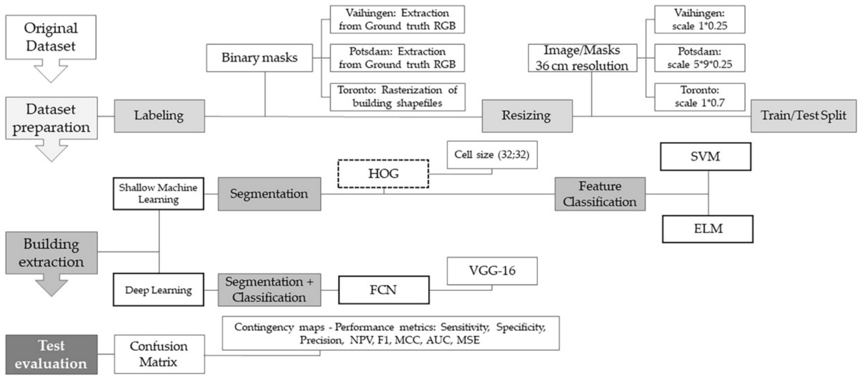
2.1. Overview
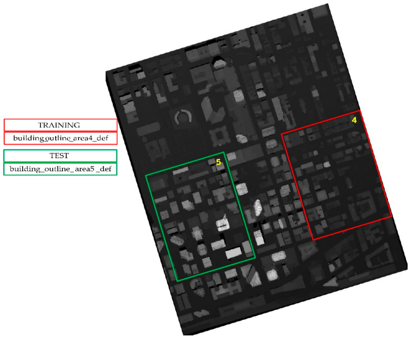
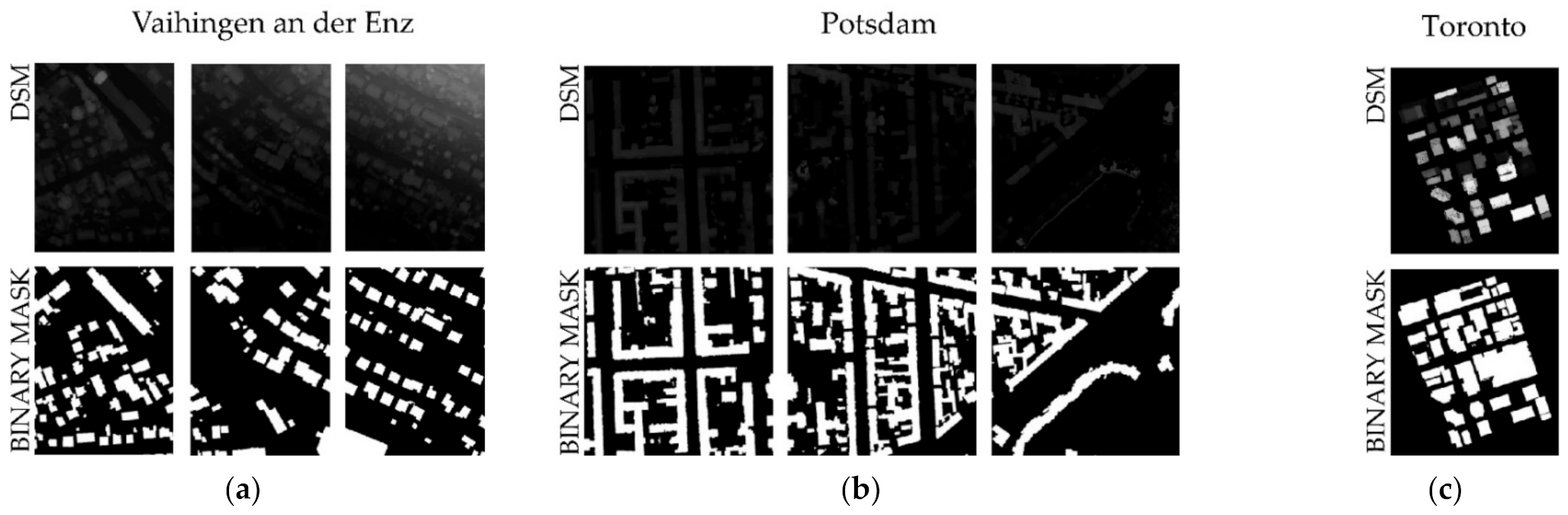
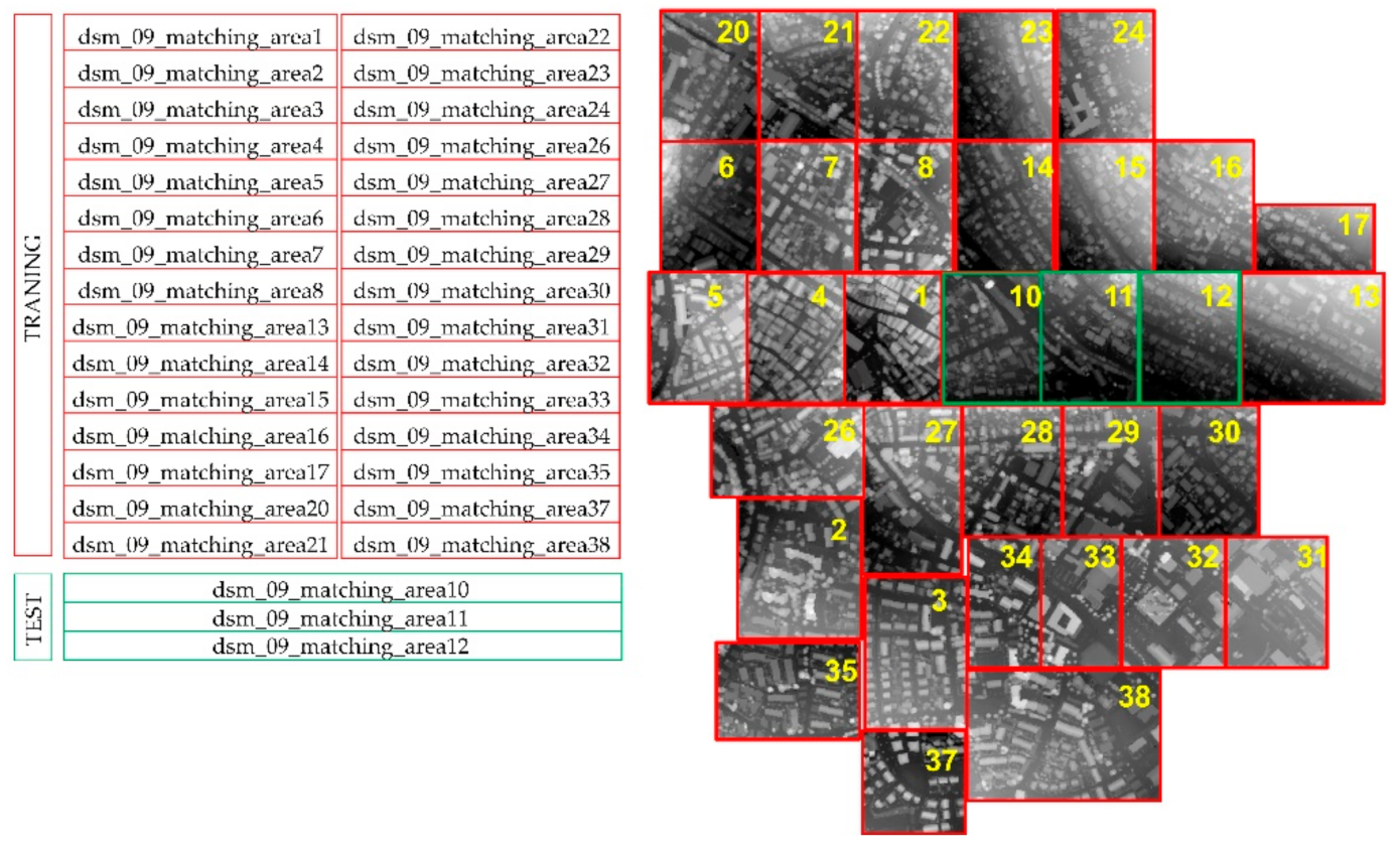
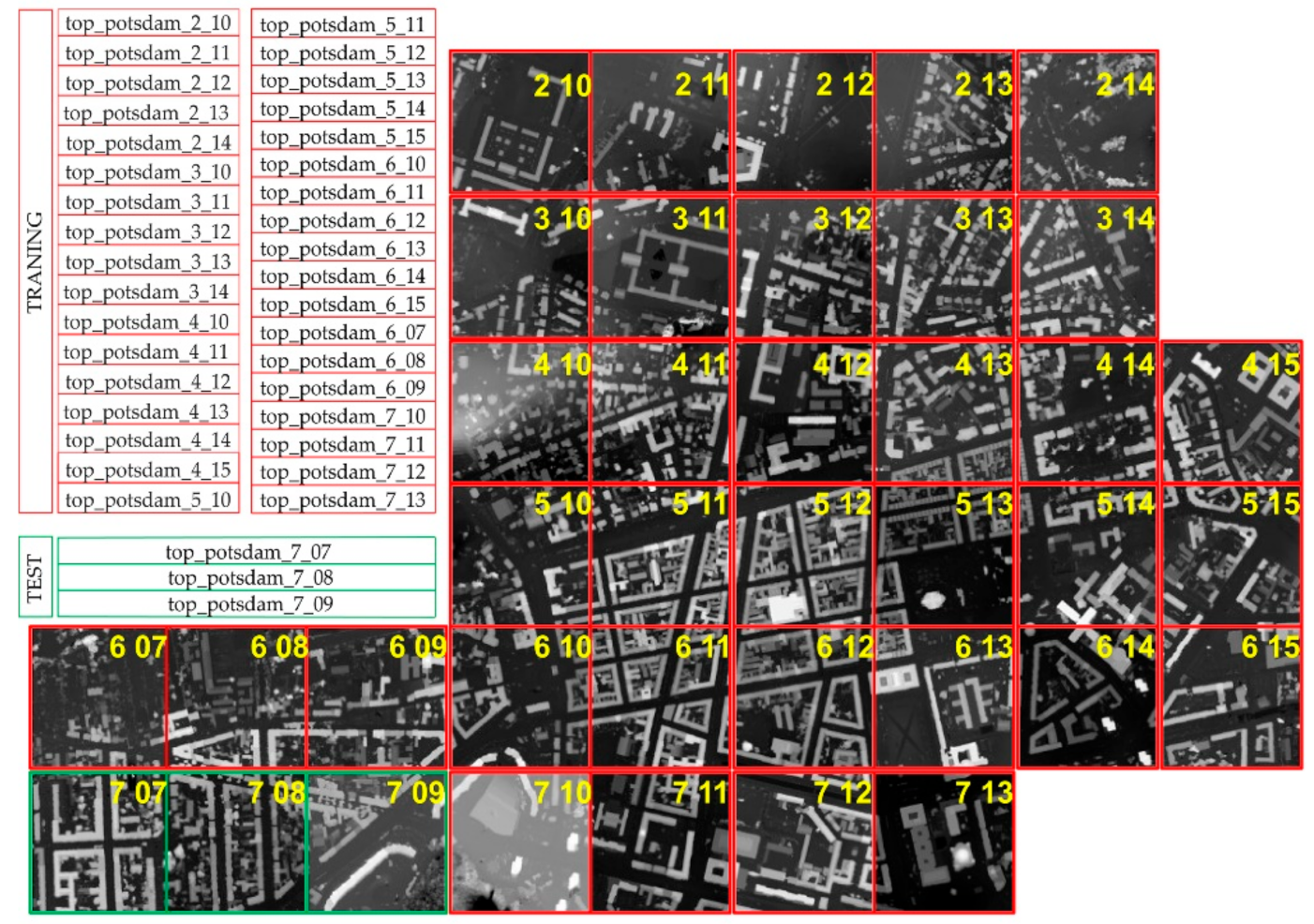
2.2. Dataset Description
2.3. Models’ Implementation and Training
2.3.1. Shallow ML-Based Building Detection
2.3.2. DL-Based Building Detection
2.4. Test Evaluation
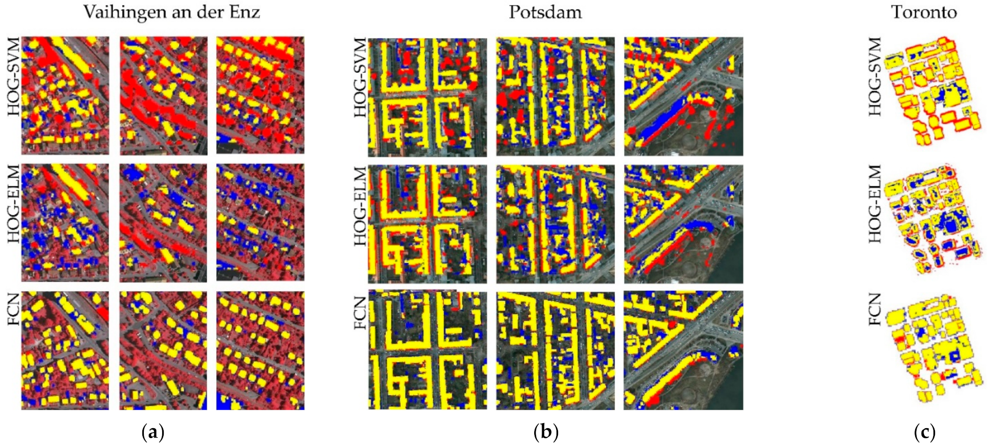
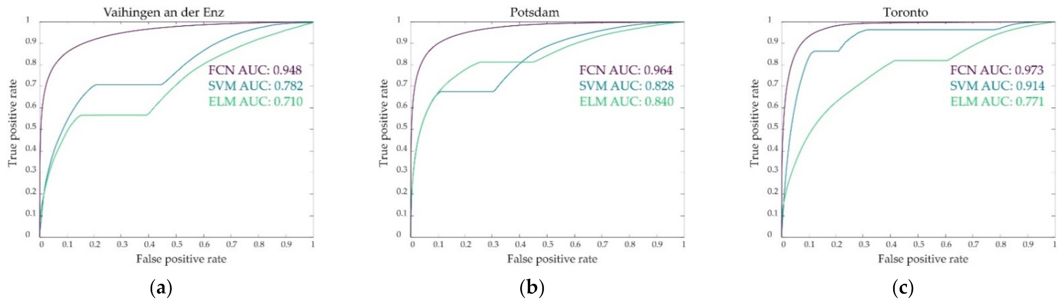
3. Results
4. Discussion
5. Conclusions
Author Contributions
Funding
Institutional Review Board Statement
Informed Consent Statement
Data Availability Statement
Conflicts of Interest
References
- Demir, I.; Koperski, K.; Lindenbaum, D.; Pang, G.; Huang, J.; Basu, S.; Hughes, F.; Tuia, D.; Raskar, R. DeepGlobe 2018: A Challenge to Parse the Earth through Satellite Images. In Proceedings of the 2018 IEEE/CVF Conference on Computer Vision and Pattern Recognition Workshops (CVPRW), Salt Lake City, UT, USA, 18–22 June 2018; IEEE: Piscataway, NJ, USA, 2018; pp. 172–17209. [Google Scholar]
- Li, L.; Liang, J.; Weng, M.; Zhu, H. A Multiple-Feature Reuse Network to Extract Buildings from Remote Sensing Imagery. Remote Sens. 2018, 10, 1350. [Google Scholar] [CrossRef] [Green Version]
- Samela, C.; Albano, R.; Sole, A.; Manfreda, S. A GIS Tool for Cost-Effective Delineation of Flood-Prone Areas. Comput. Environ. Urban Syst. 2018, 70, 43–52. [Google Scholar] [CrossRef]
- Sole, A.; Giosa, L.; Albano, R.; Cantisani, A. The laser scan data as a key element in the hydraulic flood modelling in urban areas. In Proceedings of the International Archives of the Photogrammetry, Remote Sensing and Spatial Information Sciences—(ISPRS Archive), London, UK, 29–31 May 2013; Volume XL-4/W1, pp. 65–70. [Google Scholar] [CrossRef] [Green Version]
- Tian, J.; Cui, S.; Reinartz, P. Building Change Detection Based on Satellite Stereo Imagery and Digital Surface Models. IEEE Trans. Geosci. Remote Sens. 2014, 52, 406–417. [Google Scholar] [CrossRef] [Green Version]
- Li, W.; Dong, R.; Fu, H.; Yu, L. Large-Scale Oil Palm Tree Detection from High-Resolution Satellite Images Using Two-Stage Convolutional Neural Networks. Remote Sens. 2018, 11, 11. [Google Scholar] [CrossRef] [Green Version]
- Zhang, B.; Wang, C.; Shen, Y.; Liu, Y. Fully Connected Conditional Random Fields for High-Resolution Remote Sensing Land Use/Land Cover Classification with Convolutional Neural Networks. Remote Sens. 2018, 10, 1889. [Google Scholar] [CrossRef] [Green Version]
- Audebert, N.; Le Saux, B.; Lefèvre, S. Segment-before-Detect: Vehicle Detection and Classification through Semantic Segmentation of Aerial Images. Remote Sens. 2017, 9, 368. [Google Scholar] [CrossRef] [Green Version]
- Tang, T.; Zhou, S.; Deng, A.; Lei, L.; Zou, H. Arbitrary-Oriented Vehicle Detection in Aerial Imagery with Single Convolutional Neural Networks. Remote Sens. 2017, 9, 1170. [Google Scholar] [CrossRef] [Green Version]
- Xu, Y.; Xie, Z.; Feng, Y.; Chen, Z. Road Extraction from High-Resolution Remote Sensing Imagery Using Deep Learning. Remote Sens. 2018, 10, 1461. [Google Scholar] [CrossRef] [Green Version]
- Guo, B.; Huang, X.; Zhang, F.; Sohn, G. Classification of Airborne Laser Scanning Data Using JointBoost. ISPRS J. Photogramm. Remote Sens. 2015, 100, 71–83. [Google Scholar] [CrossRef]
- Bretar, F. Feature Extraction from LiDAR Data in Urban Areas. In Topographic Laser Ranging and Scanning; Shan, J., Toth, C.K., Eds.; CRC Press: Boca Raton, FL, USA, 2017; pp. 403–420. ISBN 978-1-315-21956-1. [Google Scholar]
- Rottensteiner, F.; Sohn, G.; Gerke, M.; Wegner, J.D.; Breitkopf, U.; Jung, J. Results of the ISPRS Benchmark on Urban Object Detection and 3D Building Reconstruction. ISPRS J. Photogramm. Remote Sens. 2014, 93, 256–271. [Google Scholar] [CrossRef]
- Cheng, G.; Han, J. A Survey on Object Detection in Optical Remote Sensing Images. ISPRS J. Photogramm. Remote Sens. 2016, 117, 11–28. [Google Scholar] [CrossRef] [Green Version]
- Kass, M.; Witkin, A.; Terzopoulos, D. Snakes: Active Contour Models. Int. J. Comput. Vis. 1988, 1, 321–331. [Google Scholar] [CrossRef]
- Bypina, S.K.; Rajan, K.S. Semi-Automatic Extraction of Large and Moderate Buildings from Very High-Resolution Satellite Imagery Using Active Contour Model. In Proceedings of the 2015 IEEE International Geoscience and Remote Sensing Symposium (IGARSS), Milan, Italy, 26–31 July 2015; IEEE: Piscataway, NJ, USA, 2015; pp. 1885–1888. [Google Scholar]
- Kabolizade, M.; Ebadi, H.; Ahmadi, S. An Improved Snake Model for Automatic Extraction of Buildings from Urban Aerial Images and LiDAR Data. Comput. Environ. Urban Syst. 2010, 34, 435–441. [Google Scholar] [CrossRef]
- Liasis, G.; Stavrou, S. Building Extraction in Satellite Images Using Active Contours and Colour Features. Int. J. Remote Sens. 2016, 37, 1127–1153. [Google Scholar] [CrossRef]
- Sun, Y.; Zhang, X.; Zhao, X.; Xin, Q. Extracting Building Boundaries from High Resolution Optical Images and LiDAR Data by Integrating the Convolutional Neural Network and the Active Contour Model. Remote Sens. 2018, 10, 1459. [Google Scholar] [CrossRef] [Green Version]
- Goodfellow, I.; Bengio, Y.; Courville, A. Deep Learning; MIT Press: Cambridge, MA, USA, 2016. [Google Scholar]
- Notarangelo, N.M.; Hirano, K.; Albano, R.; Sole, A. Transfer Learning with Convolutional Neural Networks for Rainfall Detection in Single Images. Water 2021, 13, 588. [Google Scholar] [CrossRef]
- O’Mahony, N.; Campbell, S.; Carvalho, A.; Harapanahalli, S.; Hernandez, G.V.; Krpalkova, L.; Riordan, D.; Walsh, J. Deep Learning vs. Traditional Computer Vision. In Advances in Computer Vision; Arai, K., Kapoor, S., Eds.; Advances in Intelligent Systems and Computing; Springer International Publishing: Cham, Switzerland, 2020; Volume 943, pp. 128–144. ISBN 978-3-030-17794-2. [Google Scholar]
- Dalal, N.; Triggs, B. Histograms of Oriented Gradients for Human Detection. In Proceedings of the 2005 IEEE Computer Society Conference on Computer Vision and Pattern Recognition (CVPR’05), San Diego, CA, USA, 20–25 June 2005; IEEE: Piscataway, NJ, USA, 2005; Volume 1, pp. 886–893. [Google Scholar]
- Konstantinidis, D.; Stathaki, T.; Argyriou, V.; Grammalidis, N. A Probabilistic Feature Fusion for Building Detection in Satellite Images. In Proceedings of the 10th International Conference on Computer Vision Theory and Applications, Berlin, Germany, 11–14 March 2015; SCITEPRESS—Science and Technology Publications: Setúbal, Portugal, 2015; pp. 205–212. [Google Scholar]
- Ilsever, M.; Unsalan, C. Building Detection Using HOG Descriptors. In Proceedings of the 2013 6th International Conference on Recent Advances in Space Technologies (RAST), Istanbul, Turkey, 12–14 June 2013; IEEE: Piscataway, NJ, USA, 2013; pp. 115–119. [Google Scholar]
- Cheng, G.; Han, J.; Zhou, P.; Guo, L. Scalable Multi-Class Geospatial Object Detection in High-Spatial-Resolution Remote Sensing Images. In Proceedings of the 2014 IEEE Geoscience and Remote Sensing Symposium, Quebec City, QC, Canada, 13–18 July 2014; IEEE: Piscataway, NJ, USA, 2014; pp. 2479–2482. [Google Scholar]
- Tuermer, S.; Kurz, F.; Reinartz, P.; Stilla, U. Airborne Vehicle Detection in Dense Urban Areas Using HoG Features and Disparity Maps. IEEE J. Sel. Top. Appl. Earth Obs. Remote Sens. 2013, 6, 2327–2337. [Google Scholar] [CrossRef]
- Turker, M.; Koc-San, D. Building Extraction from High-Resolution Optical Spaceborne Images Using the Integration of Support Vector Machine (SVM) Classification, Hough Transformation and Perceptual Grouping. Int. J. Appl. Earth Obs. Geoinf. 2015, 34, 58–69. [Google Scholar] [CrossRef]
- Krupinski, M.; Lewiński, S.; Malinowski, R. One Class SVM for Building Detection on Sentinel-2 Images. In Proceedings of the Photonics Applications in Astronomy, Communications, Industry, and High-Energy Physics Experiments, Wilga, Poland, 6 November 2019; Romaniuk, R.S., Linczuk, M., Eds.; SPIE: Bellingham, WA, USA, 2019; p. 6. [Google Scholar]
- Mountrakis, G.; Im, J.; Ogole, C. Support Vector Machines in Remote Sensing: A Review. ISPRS J. Photogramm. Remote Sens. 2011, 66, 247–259. [Google Scholar] [CrossRef]
- Lari, Z.; Ebadi, H. Automated Building Extraction from High-Resolution Satellite Imagery Using Spectral and Structural Information Based on Artificial Neural Networks. In Proceedings of the International Archives of Photogrammetry, Remote Sensing and Spatial Information Sciences, Hannover, Germany, 29 May–1 June 2007; Volume 36. [Google Scholar]
- Albano, R.; Samela, C.; Crăciun, I.; Manfreda, S.; Adamowski, J.; Sole, A.; Sivertun, Å.; Ozunu, A. Large Scale Flood Risk Mapping in Data Scarce Environments: An Application for Romania. Water 2020, 12, 1834. [Google Scholar] [CrossRef]
- Wang, P.; Zhang, X.; Hao, Y. A Method Combining CNN and ELM for Feature Extraction and Classification of SAR Image. J. Sens. 2019, 2019, 1–8. [Google Scholar] [CrossRef]
- Nahhas, F.H.; Shafri, H.Z.M.; Sameen, M.I.; Pradhan, B.; Mansor, S. Deep Learning Approach for Building Detection Using LiDAR–Orthophoto Fusion. J. Sens. 2018, 2018, 1–12. [Google Scholar] [CrossRef] [Green Version]
- Maltezos, E.; Doulamis, A.; Doulamis, N.; Ioannidis, C. Building Extraction from LiDAR Data Applying Deep Convolutional Neural Networks. IEEE Geosci. Remote Sens. Lett. 2019, 16, 155–159. [Google Scholar] [CrossRef]
- Vakalopoulou, M.; Karantzalos, K.; Komodakis, N.; Paragios, N. Building Detection in Very High Resolution Multispectral Data with Deep Learning Features. In Proceedings of the 2015 IEEE International Geoscience and Remote Sensing Symposium (IGARSS), Milan, Italy, 26–31 July 2015; IEEE: Piscataway, NJ, USA, 2015; pp. 1873–1876. [Google Scholar]
- Diakogiannis, F.I.; Waldner, F.; Caccetta, P.; Wu, C. ResUNet-a: A Deep Learning Framework for Semantic Segmentation of Remotely Sensed Data. ISPRS J. Photogramm. Remote Sens. 2020, 162, 94–114. [Google Scholar] [CrossRef] [Green Version]
- Zhong, Z.; Li, J.; Cui, W.; Jiang, H. Fully Convolutional Networks for Building and Road Extraction: Preliminary Results. In Proceedings of the 2016 IEEE International Geoscience and Remote Sensing Symposium (IGARSS), Beijing, China, 10–15 July 2016; IEEE: Piscataway, NJ, USA, 2016; pp. 1591–1594. [Google Scholar]
- Xu, Y.; Wu, L.; Xie, Z.; Chen, Z. Building Extraction in Very High Resolution Remote Sensing Imagery Using Deep Learning and Guided Filters. Remote Sens. 2018, 10, 144. [Google Scholar] [CrossRef] [Green Version]
- Fu, G.; Liu, C.; Zhou, R.; Sun, T.; Zhang, Q. Classification for High Resolution Remote Sensing Imagery Using a Fully Convolutional Network. Remote Sens. 2017, 9, 498. [Google Scholar] [CrossRef] [Green Version]
- Maggiori, E.; Tarabalka, Y.; Charpiat, G.; Alliez, P. Convolutional Neural Networks for Large-Scale Remote-Sensing Image Classification. IEEE Trans. Geosci. Remote Sens. 2017, 55, 645–657. [Google Scholar] [CrossRef] [Green Version]
- Shrestha, S.; Vanneschi, L. Improved Fully Convolutional Network with Conditional Random Fields for Building Extraction. Remote Sens. 2018, 10, 1135. [Google Scholar] [CrossRef] [Green Version]
- Audebert, N.; Saux, B.L.; Lefèvre, S. Semantic Segmentation of Earth Observation Data Using Multimodal and Multi-Scale Deep Networks. arXiv 2016, arXiv:1609.06846. [Google Scholar]
- Arefi, H.; Reinartz, P. Building Reconstruction Using DSM and Orthorectified Images. Remote Sens. 2013, 5, 1681–1703. [Google Scholar] [CrossRef] [Green Version]
- Protopapadakis, E.; Doulamis, A.; Doulamis, N.; Maltezos, E. Stacked Autoencoders Driven by Semi-Supervised Learning for Building Extraction from near Infrared Remote Sensing Imagery. Remote Sens. 2021, 13, 371. [Google Scholar] [CrossRef]
- Chorowski, J.; Wang, J.; Zurada, J.M. Review and Performance Comparison of SVM- and ELM-Based Classifiers. Neurocomputing 2014, 128, 507–516. [Google Scholar] [CrossRef]
- Huang, G.B.; Zhou, H.; Ding, X.; Zhang, R. Extreme Learning Machine for Regression and Multiclass Classification. IEEE Trans. Syst. Man Cybern. B 2012, 42, 513–529. [Google Scholar] [CrossRef] [PubMed] [Green Version]
- Yang, L.; Lyu, K.; Li, H.; Liu, Y. Building Climate Zoning in China Using Supervised Classification-Based Machine Learning. Build. Environ. 2020, 171, 106663. [Google Scholar] [CrossRef]
- Khan, M.A. HCRNNIDS: Hybrid Convolutional Recurrent Neural Network-Based Network Intrusion Detection System. Processes 2021, 9, 834. [Google Scholar] [CrossRef]
- Long, J.; Shelhamer, E.; Darrell, T. Fully Convolutional Networks for Semantic Segmentation. In Proceedings of the 2015 IEEE Conference on Computer Vision and Pattern Recognition (CVPR), Boston, MA, USA, 7–12 June 2015; IEEE: Piscataway, NJ, USA, 2015; pp. 3431–3440. [Google Scholar]
- Kotsiantis, S. Supervised Machine Learning: A Review of Classification Techniques. Informatica 2007, 31, 249–268. [Google Scholar]
- Minaee, S.; Boykov, Y.; Porikli, F.; Plaza, A.; Kehtarnavaz, N.; Terzopoulos, D. Image Segmentation Using Deep Learning: A Survey. arXiv 2020, arXiv:2001.05566. [Google Scholar]
- Rottensteiner, F.; Sohn, G.; Jung, J.; Gerke, M.; Baillard, C.; Benitez, S.; Breitkopf, U. The ISPRS Benchmark on Urban Object Classification and 3d Building Reconstruction. ISPRS Ann. Photogramm. Remote Sens. Spat. Inf. Sci. I-3 2012, 1, 293–298. [Google Scholar] [CrossRef] [Green Version]
- Champion, N.; Rottensteiner, F.; Matikainen, L.; Liang, X.; Hyyppä, J.; Olsen, B. A Test of Automatic Building Change Detection Approaches. In Proceedings of the CMRT09, Paris, France, 3–4 September 2009. [Google Scholar]
- Kaartinen, H.; Hyyppä, J.; Gülch, E.; Vosselman, G.; Hyyppä, H.; Matikainen, L.; Hofmann, A.; Mäder, U.; Persson, Å.; Söderman, U.; et al. Accuracy of 3D City Models: EuroSDR Comparison. Int. Arch. Photogramm. Remote Sens. Spat. Inf. Sci. 2005, 36, 227–232. [Google Scholar]
- Mayer, H.; Hinz, S.; Bacher, U.; Baltsavias, E. A Test of Automatic Road Extraction Approaches. Int. Arch. Photogramm. Remote Sens. Spat. Inf. Sci. 2006, 36, 209–214. [Google Scholar]
- Cramer, M. The DGPF-Test on Digital Airborne Camera Evaluation Overview and Test Design. PFG Photogramm. Fernerkund. Geoinf. 2010, 2010, 73–82. [Google Scholar] [CrossRef]
- Haala, N.; Cramer, M.; Jacobsen, K. The German Camera Evaluation Project-Results from the Geometry Group. In Proceedings of the International Archives of the Photogrammetry, Remote Sensing and Spatial Information Sciences: [2010 Canadian Geomatics Conference and Symposium of Commission I, ISPRS Convergence in Geomatics-Shaping Canada’s Competitive Landscape], Calgary, AB, Canada, 15–18 June 2010; Nr. Part 1; Copernicus GmbH: Göttingen, Germany, 2010; Volume 38. [Google Scholar]
- Albano, R. Investigation on Roof Segmentation for 3D Building Reconstruction from Aerial LIDAR Point Clouds. Appl. Sci. 2019, 9, 4674. [Google Scholar] [CrossRef] [Green Version]
- Cristianini, N.; Shawe-Taylor, J. An Introduction to Support Vector Machines and Other Kernel-Based Learning Methods, 1st ed.; Cambridge University Press: Cambridge, UK, 2000; ISBN 978-0-521-78019-3. [Google Scholar]
- Durst, N.J.; Sullivan, E.; Huang, H.; Park, H. Building Footprint-Derived Landscape Metrics for the Identification of Informal Subdivisions and Manufactured Home Communities: A Pilot Application in Hidalgo County, Texas. Land Use Policy 2021, 101, 105158. [Google Scholar] [CrossRef]
- Foody, G.M.; Mathur, A. A Relative Evaluation of Multiclass Image Classification by Support Vector Machines. IEEE Trans. Geosci. Remote Sens. 2004, 42, 1335–1343. [Google Scholar] [CrossRef] [Green Version]
- Huang, C.; Davis, L.S.; Townshend, J.R.G. An Assessment of Support Vector Machines for Land Cover Classification. Int. J. Remote Sens. 2002, 23, 725–749. [Google Scholar] [CrossRef]
- Schölkopf, B.; Smola, A.J.; Bach, F. Learning with Kernels: Support Vector Machines, Regularization, Optimization, and Beyond; MIT Press: Cambridge, MA, USA, 2002. [Google Scholar]
- Guenther, N.; Schonlau, M. Support Vector Machines. Stata J. 2016, 16, 917–937. [Google Scholar] [CrossRef] [Green Version]
- Vapnik, V. The Nature of Statistical Learning Theory; Springer Science & Business Media: Berlin, Germany, 2013. [Google Scholar]
- Wang, L. Support Vector Machines: Theory and Applications; Springer Science & Business Media: Berlin, Germany, 2005; Volume 177. [Google Scholar]
- Fan, R.-E.; Chen, P.-H.; Lin, C.-J. Working Set Selection Using Second Order Information for Training Support Vector Machines. J. Mach. Learn. Res. 2005, 6, 1889–1918. [Google Scholar] [CrossRef]
- Ertuğrul, Ö.F.; Kaya, Y. A Detailed Analysis on Extreme Learning Machine and Novel Approaches Based on ELM. Am. J. Comput. Sci. Eng. 2014, 1, 43–50. [Google Scholar]
- Huang, G.B.; Zhu, Q.Y.; Siew, C.K. Extreme Learning Machine: A New Learning Scheme of Feedforward Neural Networks. In Proceedings of the 2004 IEEE International Joint Conference on Neural Networks (IEEE Cat. No.04CH37541), Budapest, Hungary, 25–29 July 2004; IEEE: Piscataway, NJ, USA, 2004; Volume 2, pp. 985–990. [Google Scholar]
- Huang, G.-B. An Insight into Extreme Learning Machines: Random Neurons, Random Features and Kernels. Cogn. Comput. 2014, 6, 376–390. [Google Scholar] [CrossRef]
- Liu, X.; Gao, C.; Li, P. A Comparative Analysis of Support Vector Machines and Extreme Learning Machines. Neural Netw. 2012, 33, 58–66. [Google Scholar] [CrossRef]
- Bischke, B.; Helber, P.; Folz, J.; Borth, D.; Dengel, A. Multi-Task Learning for Segmentation of Building Footprints with Deep Neural Networks. arXiv 2017, arXiv:1709.05932. [Google Scholar]
- Li, Y.; He, B.; Long, T.; Bai, X. Evaluation the Performance of Fully Convolutional Networks for Building Extraction Compared with Shallow Models. In Proceedings of the 2017 IEEE International Geoscience and Remote Sensing Symposium (IGARSS), Fort Worth, TX, USA, 23–28 July 2017; IEEE: Piscataway, NJ, USA, 2017; pp. 850–853. [Google Scholar]
- Liu, T.; Abd-Elrahman, A. An Object-Based Image Analysis Method for Enhancing Classification of Land Covers Using Fully Convolutional Networks and Multi-View Images of Small Unmanned Aerial System. Remote Sens. 2018, 10, 457. [Google Scholar] [CrossRef] [Green Version]
- Krizhevsky, A.; Sutskever, I.; Hinton, G.E. Imagenet Classification with Deep Convolutional Neural Networks. Adv. Neural Inf. Process. Syst. 2012, 25, 1097–1105. [Google Scholar] [CrossRef]
- Simonyan, K.; Zisserman, A. Very Deep Convolutional Networks for Large-Scale Image Recognition. arXiv 2014, arXiv:1409.1556. [Google Scholar]
- Murphy, K.P. Machine Learning: A Probabilistic Perspective; Adaptive Computation and Machine LEARNING series; MIT Press: Cambridge, MA, USA, 2012; ISBN 978-0-262-01802-9. [Google Scholar]
- Zheng, A. Evaluating Machine Learning Models; O’Reilly Media, Inc.: Sebastopol, CA, USA, 2015; ISBN 978-1-4920-4875-6. [Google Scholar]
- Scarpino, S.; Albano, R.; Cantisani, A.; Mancusi, L.; Sole, A.; Milillo, G. Multitemporal SAR Data and 2D Hydrodynamic Model Flood Scenario Dynamics Assessment. IJGI 2018, 7, 105. [Google Scholar] [CrossRef] [Green Version]
- Albano, R.; Mancusi, L.; Adamowski, J.; Cantisani, A.; Sole, A. A GIS Tool for Mapping Dam-Break Flood Hazards in Italy. IJGI 2019, 8, 250. [Google Scholar] [CrossRef] [Green Version]
- Powers, D.M.W. Evaluation: From Precision, Recall and F-Measure to ROC, Informedness, Markedness and Correlation. arXiv 2020, arXiv:2010.16061. [Google Scholar]
- Chicco, D.; Jurman, G. The Advantages of the Matthews Correlation Coefficient (MCC) over F1 Score and Accuracy in Binary Classification Evaluation. BMC Genom. 2020, 21, 6. [Google Scholar] [CrossRef] [Green Version]
- Hosmer, D.W.; Lemeshow, S. Applied Logistic Regression; John Wiley & Sons: New York, NY, USA; Toronto, ON, Canada, 2005; ISBN 978-0-471-72214-4. [Google Scholar]
- Liu, T.; Abd-Elrahman, A.; Morton, J.; Wilhelm, V.L. Comparing Fully Convolutional Networks, Random Forest, Support Vector Machine, and Patch-Based Deep Convolutional Neural Networks for Object-Based Wetland Mapping Using Images from Small Unmanned Aircraft System. GISci. Remote Sens. 2018, 55, 243–264. [Google Scholar] [CrossRef]
- Yang, Y.; Zhou, X.; Liu, Y.; Hu, Z.; Ding, F. Wood Defect Detection Based on Depth Extreme Learning Machine. Appl. Sci. 2020, 10, 7488. [Google Scholar] [CrossRef]
- Chen, T.-L.; Chiu, H.-W.; Lin, Y.-F. How Do East and Southeast Asian Cities Differ from Western Cities? A Systematic Review of the Urban Form Characteristics. Sustainability 2020, 12, 2423. [Google Scholar] [CrossRef] [Green Version]
- Uuemaa, E.; Ahi, S.; Montibeller, B.; Muru, M.; Kmoch, A. Vertical Accuracy of Freely Available Global Digital Elevation Models (ASTER, AW3D30, MERIT, TanDEM-X, SRTM, and NASADEM). Remote Sens. 2020, 12, 3482. [Google Scholar] [CrossRef]


| Sensitivity | Specificity | Precision | NPV | F1 Score | MSE | MCC | AUC | ||
|---|---|---|---|---|---|---|---|---|---|
| HOG-SVM | Vaihingen | 0.773 | 0.767 | 0.446 | 0.933 | 0.566 | 0.044 | 0.657 | 0.782 |
| Potsdam | 0.737 | 0.876 | 0.718 | 0.886 | 0.728 | 0.079 | 0.620 | 0.828 | |
| Toronto | 0.887 | 0.871 | 0.742 | 0.949 | 0.808 | 0.033 | 0.826 | 0.914 | |
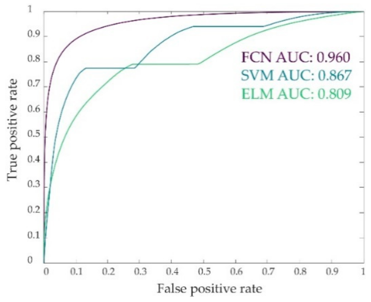
| Total | 0.817 | 0.854 | 0.687 | 0.923 | 0.746 | 0.058 | 0.725 | 0.867 | |
| HOG-ELM | Vaihingen | 0.415 | 0.935 | 0.608 | 0.868 | 0.493 | 0.114 | 0.513 | 0.710 |
| Potsdam | 0.720 | 0.888 | 0.735 | 0.881 | 0.727 | 0.084 | 0.620 | 0.840 | |
| Toronto | 0.654 | 0.909 | 0.749 | 0.863 | 0.698 | 0.102 | 0.644 | 0.771 | |
| Total | 0.653 | 0.906 | 0.731 | 0.870 | 0.690 | 0.099 | 0.626 | 0.809 | |
| FCN | Vaihingen | 0.741 | 0.966 | 0.872 | 0.923 | 0.801 | 0.061 | 0.833 | 0.948 |
| Potsdam | 0.801 | 0.948 | 0.784 | 0.899 | 0.792 | 0.060 | 0.834 | 0.964 | |
| Toronto | 0.834 | 0.947 | 0.877 | 0.925 | 0.855 | 0.052 | 0.821 | 0.973 | |
| Total | 0.785 | 0.956 | 0.883 | 0.914 | 0.831 | 0.063 | 0.834 | 0.960 | |
| Method | Algorithm | Advantages | Disadvantages |
|---|---|---|---|
| HOG-SVM | [60] |
|
|
| HOG-ELM | [70] |
|
|
| FCN | [50] |
|
|
Publisher’s Note: MDPI stays neutral with regard to jurisdictional claims in published maps and institutional affiliations. |
© 2021 by the authors. Licensee MDPI, Basel, Switzerland. This article is an open access article distributed under the terms and conditions of the Creative Commons Attribution (CC BY) license (https://creativecommons.org/licenses/by/4.0/).
Share and Cite
Notarangelo, N.M.; Mazzariello, A.; Albano, R.; Sole, A. Comparing Three Machine Learning Techniques for Building Extraction from a Digital Surface Model. Appl. Sci. 2021, 11, 6072. https://doi.org/10.3390/app11136072
Notarangelo NM, Mazzariello A, Albano R, Sole A. Comparing Three Machine Learning Techniques for Building Extraction from a Digital Surface Model. Applied Sciences. 2021; 11(13):6072. https://doi.org/10.3390/app11136072
Chicago/Turabian StyleNotarangelo, Nicla Maria, Arianna Mazzariello, Raffaele Albano, and Aurelia Sole. 2021. "Comparing Three Machine Learning Techniques for Building Extraction from a Digital Surface Model" Applied Sciences 11, no. 13: 6072. https://doi.org/10.3390/app11136072
APA StyleNotarangelo, N. M., Mazzariello, A., Albano, R., & Sole, A. (2021). Comparing Three Machine Learning Techniques for Building Extraction from a Digital Surface Model. Applied Sciences, 11(13), 6072. https://doi.org/10.3390/app11136072