
Combined Geodetic and Seismological Study of the December 2020 Mw = 4.6 Thiva (Central Greece) Shallow Earthquake

 ,
,  ,
,  ,
,  and
and 
Abstract
1. Introduction
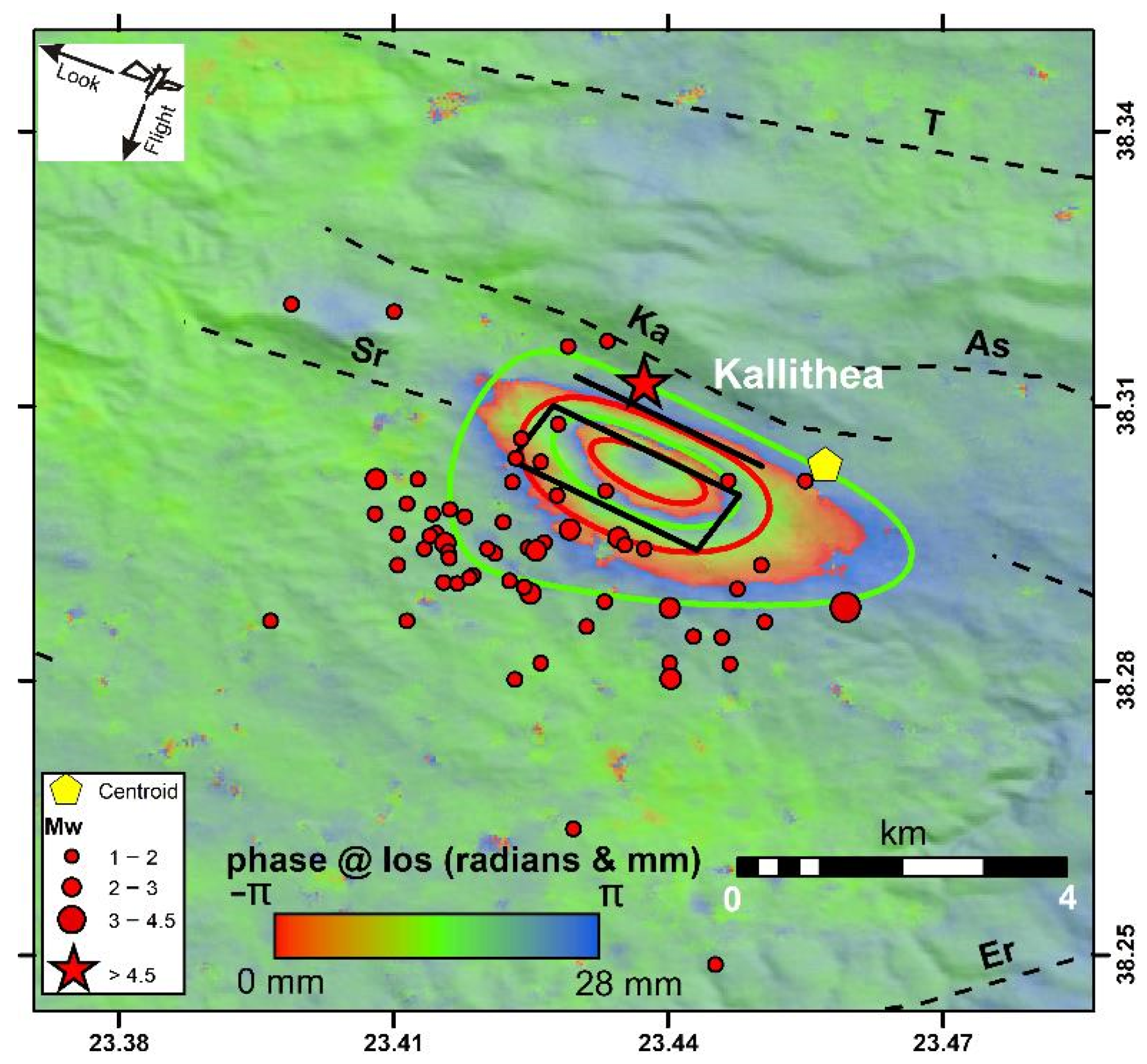
2. Geodetic Methods
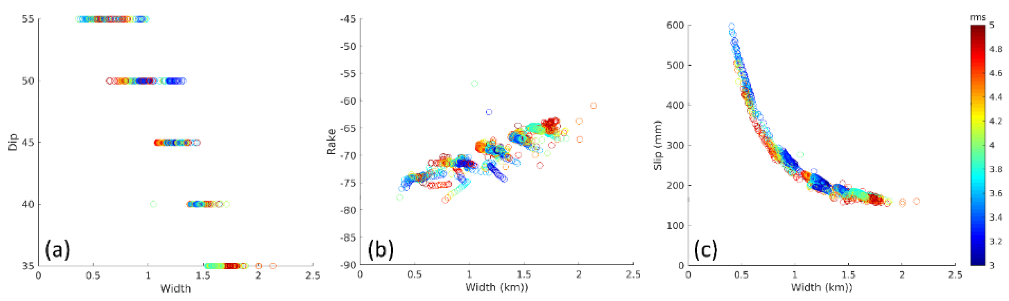
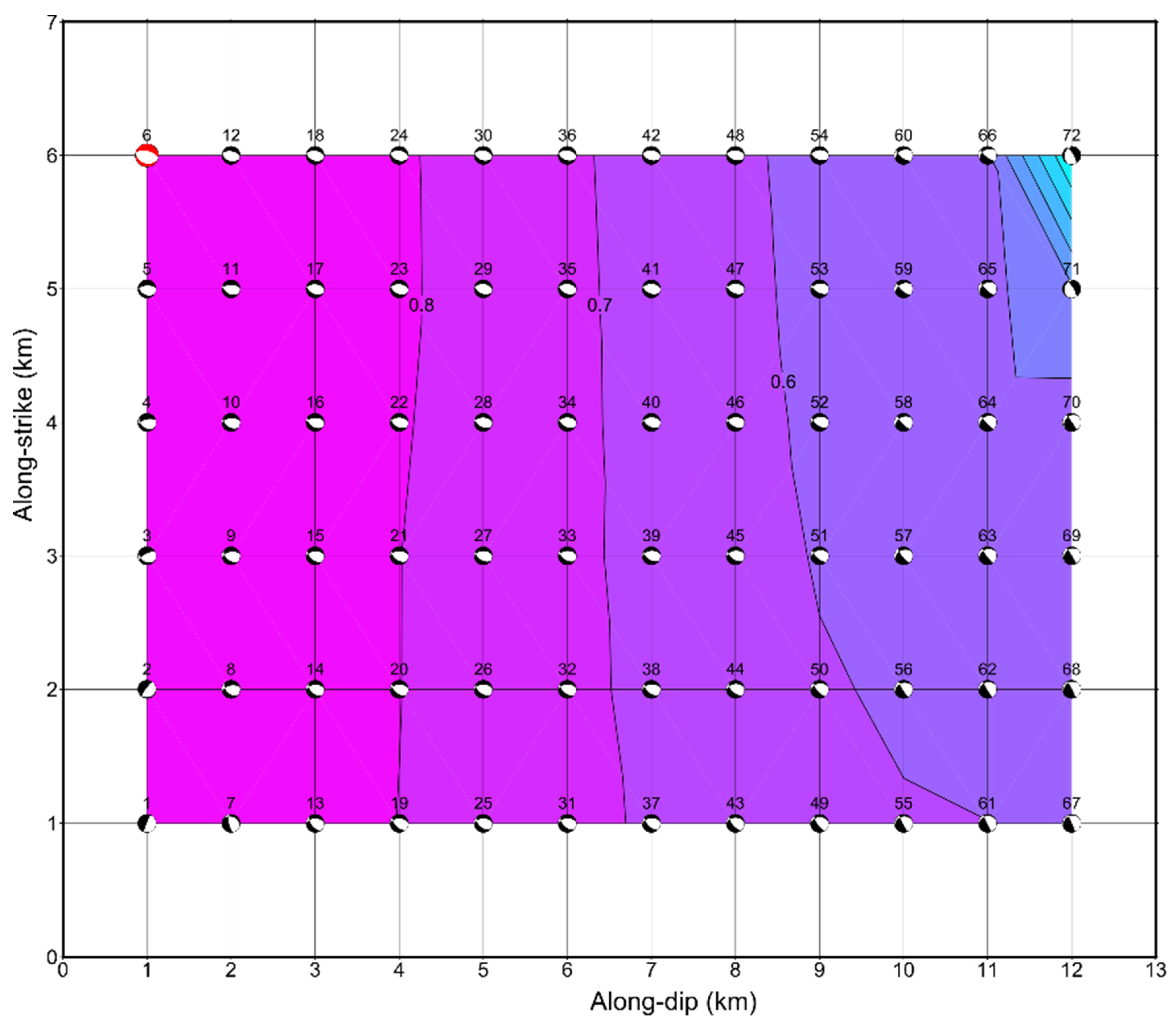
3. Inversion of Geodetic Data—Fault Model
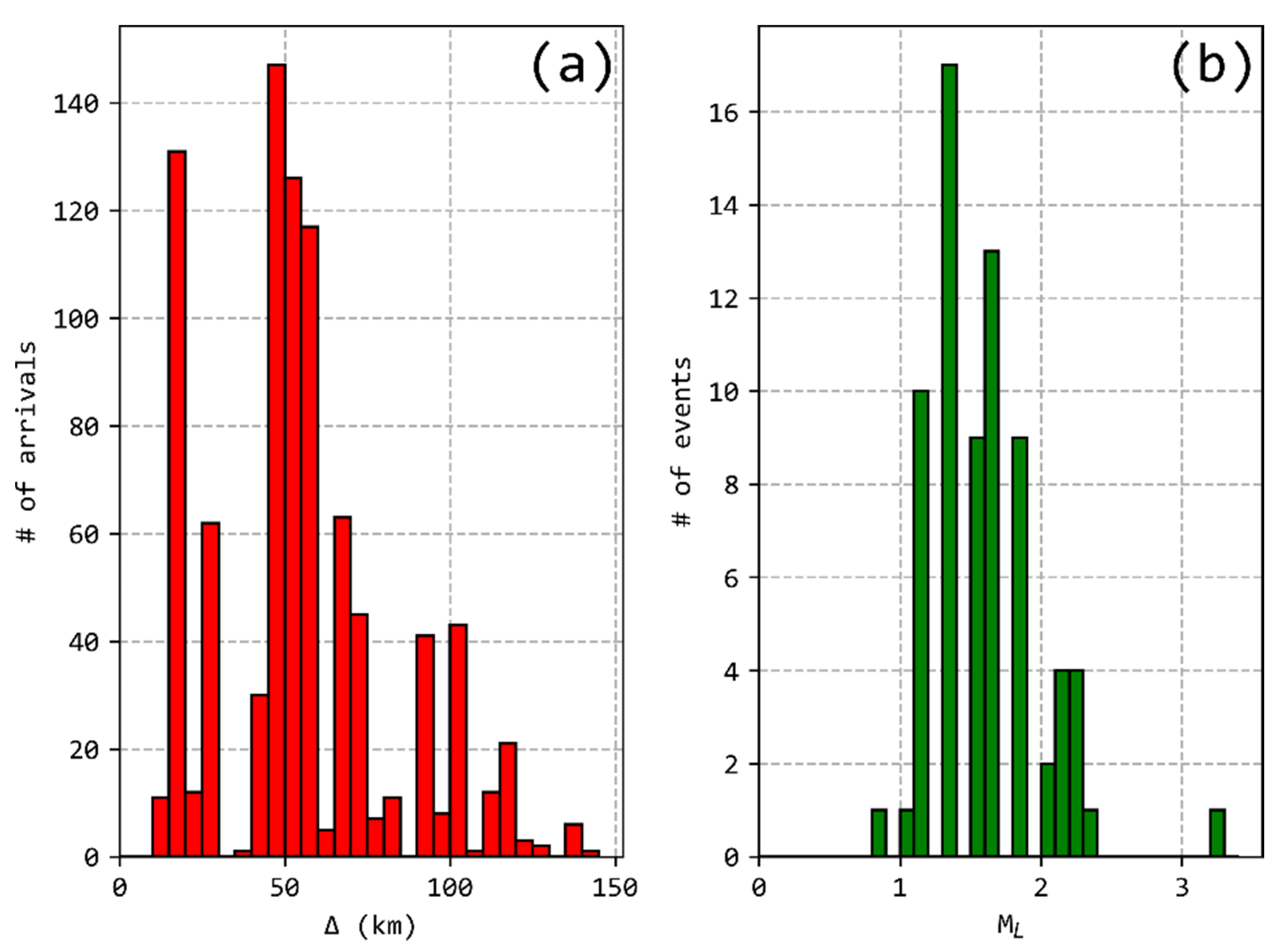
4. Seismological Methods
5. Discussion
6. Conclusions
Author Contributions
Funding
Institutional Review Board Statement
Informed Consent Statement
Data Availability Statement
Acknowledgments
Conflicts of Interest
Appendix A. Geodetic Methods Details


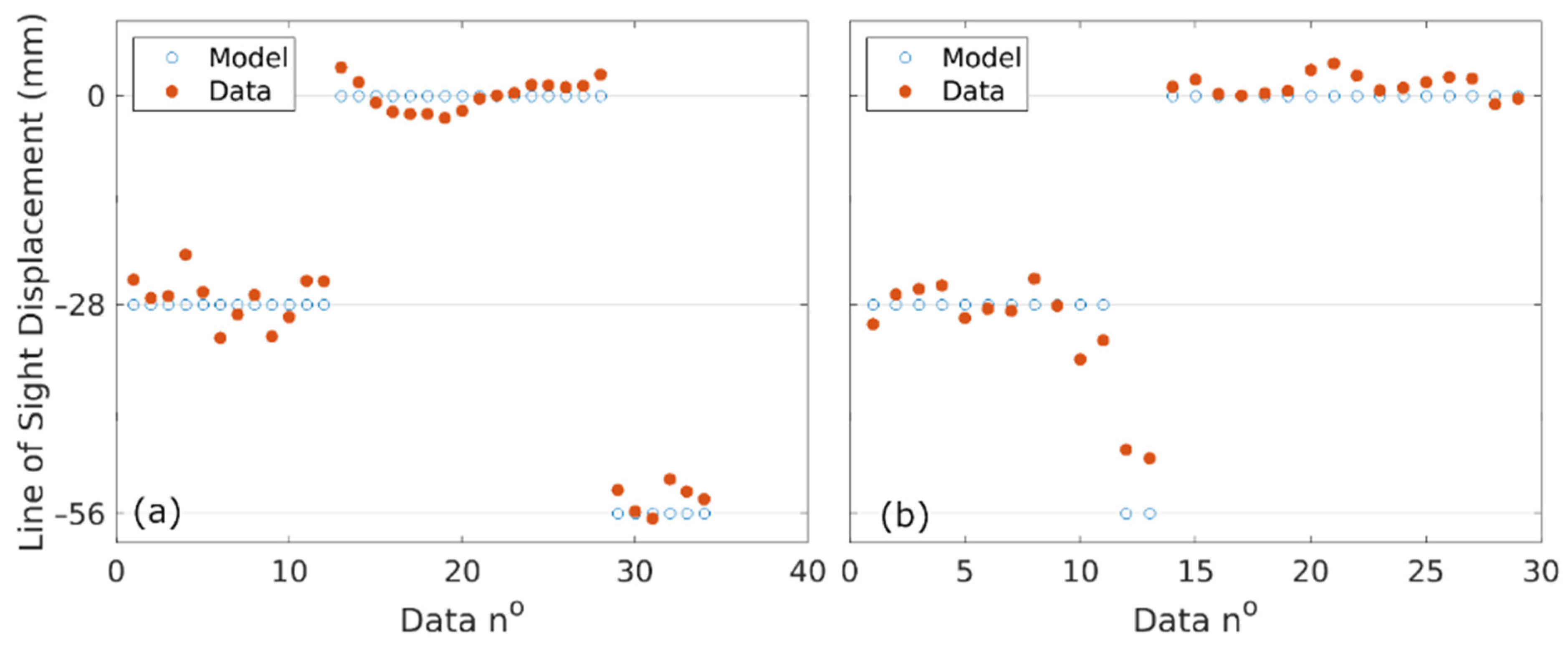
| Ascending Track 102 | Descending Track 102 | |||||||
|---|---|---|---|---|---|---|---|---|
| Pick No. | Long. (°E) | Lat. (°N) | Picked Value (mm) | Model (mm) | Long. (°E) | Lat. (°N) | Picked Value (mm) | Model (mm) |
| 1 | 23.42948 | 38.29764 | −28 | −24.65 | 23.43559 | 38.29896 | −28 | −30.6 |
| 2 | 23.42241 | 38.30126 | −28 | −27.1 | 23.44081 | 38.29666 | −28 | −26.66 |
| 3 | 23.41931 | 38.30648 | −28 | −26.86 | 23.44709 | 38.29781 | −28 | −25.91 |
| 4 | 23.41975 | 38.31011 | −28 | −21.29 | 23.44665 | 38.3025 | −28 | −25.4 |
| 5 | 23.42462 | 38.31091 | −28 | −26.33 | 23.44187 | 38.30489 | −28 | −29.78 |
| 6 | 23.42966 | 38.30967 | −28 | −32.45 | 23.43745 | 38.3071 | −28 | −28.54 |
| 7 | 23.43577 | 38.30728 | −28 | −29.29 | 23.43364 | 38.30834 | −28 | −28.84 |
| 8 | 23.44116 | 38.30436 | −28 | −26.68 | 23.42975 | 38.30931 | −28 | −24.49 |
| 9 | 23.44293 | 38.30153 | −28 | −32.24 | 23.42798 | 38.30772 | −28 | −28.14 |
| 10 | 23.44222 | 38.29826 | −28 | −29.64 | 23.42966 | 38.30454 | −28 | −35.32 |
| 11 | 23.43992 | 38.29657 | −28 | −24.78 | 23.43161 | 38.30171 | −28 | −32.77 |
| 12 | 23.43506 | 38.29649 | −28 | −24.84 | 23.43656 | 38.30445 | −56 | −47.43 |
| 13 | 23.42825 | 38.28428 | 0 | 3.83 | 23.4378 | 38.30356 | −56 | −48.61 |
| 14 | 23.41329 | 38.28844 | 0 | 1.83 | 23.43338 | 38.28746 | 0 | 1.24 |
| 15 | 23.4048 | 38.29516 | 0 | −0.88 | 23.44444 | 38.28481 | 0 | 2.17 |
| 16 | 23.39967 | 38.30259 | 0 | −2.14 | 23.45921 | 38.28799 | 0 | 0.22 |
| 17 | 23.39914 | 38.30949 | 0 | −2.41 | 23.46646 | 38.29127 | 0 | 0.07 |
| 18 | 23.40356 | 38.31542 | 0 | −2.43 | 23.46885 | 38.29702 | 0 | 0.32 |
| 19 | 23.41214 | 38.31763 | 0 | −2.94 | 23.46098 | 38.30224 | 0 | 0.68 |
| 20 | 23.42011 | 38.31878 | 0 | −2 | 23.45319 | 38.30799 | 0 | 3.49 |
| 21 | 23.43258 | 38.31604 | 0 | −0.37 | 23.44426 | 38.31241 | 0 | 4.38 |
| 22 | 23.447 | 38.31126 | 0 | 0.03 | 23.43577 | 38.31621 | 0 | 2.69 |
| 23 | 23.45452 | 38.30693 | 0 | 0.4 | 23.42542 | 38.31913 | 0 | 0.76 |
| 24 | 23.46142 | 38.30029 | 0 | 1.45 | 23.41595 | 38.32126 | 0 | 1.08 |
| 25 | 23.46461 | 38.29206 | 0 | 1.43 | 23.41064 | 38.31843 | 0 | 1.82 |
| 26 | 23.46054 | 38.28578 | 0 | 1.14 | 23.41055 | 38.31453 | 0 | 2.49 |
| 27 | 23.45213 | 38.28277 | 0 | 1.32 | 23.41303 | 38.30701 | 0 | 2.3 |
| 28 | 23.44019 | 38.28224 | 0 | 2.85 | 23.4186 | 38.29861 | 0 | −1.15 |
| 29 | 23.43311 | 38.30162 | −56 | −52.85 | 23.42506 | 38.2918 | 0 | −0.4 |
| 30 | 23.42948 | 38.30356 | −56 | −55.72 | ||||
| 31 | 23.42957 | 38.30639 | −56 | −56.66 | ||||
| 32 | 23.43355 | 38.30586 | −56 | −51.44 | ||||
| 33 | 23.43621 | 38.30374 | −56 | −53.07 | ||||
| 34 | 23.43532 | 38.30171 | −56 | −54.08 | ||||


Appendix B. Quality of Seismological Solutions


References
- Makropoulos, K.; Kaviris, G.; Kouskouna, V. An updated and extended earthquake catalogue for Greece and adjacent areas since 1900. Nat. Hazards Earth Syst. Sci. 2012, 12. [Google Scholar] [CrossRef]
- Stewart, I.S.; Piccardi, L. Seismic faults and sacred sanctuaries in Aegean antiquity. Proc. Geol. Assoc. 2017, 128. [Google Scholar] [CrossRef]
- Nur, A.; Cline, E.H. Poseidon’s horses: Plate tectonics and earthquake storms in the Late Bronze Age Aegean and Eastern Mediterranean. J. Archaeol. Sci. 2000, 27. [Google Scholar] [CrossRef]
- Papazachos, B.C.; Papazachou, C. The Earthquakes of Greece; Ziti Publications: Thessaloniki, Greek, 2003. [Google Scholar]
- Stucchi, M.; Rovida, A.; Gomez Capera, A.A.; Alexandre, P.; Camelbeeck, T.; Demircioglu, M.B.; Gasperini, P.; Kouskouna, V.; Musson, R.M.W.; Radulian, M.; et al. The SHARE European Earthquake Catalogue (SHEEC) 1000-1899. J. Seismol. 2013, 17. [Google Scholar] [CrossRef]
- Ambraseys, N.N.; Jackson, J.A. Seismicity and associated strain of central Greece between 1890 and 1988. Geophys. J. Int. 1990, 101, 663–708. [Google Scholar] [CrossRef]
- Briole, P.; Ganas, A.; Elias, P.; Dimitrov, D. The GPS velocity field of the Aegean. New observations, contribution of the earthquakes, crustal blocks model. Geophys. J. Int. 2021. [Google Scholar] [CrossRef]
- NOAFAULTS KMZ layer Version 3.0 (2020 Update). Available online: https://zenodo.org/record/4304613#.YNSWXJVR2Uk. (accessed on 1 June 2021).
- Ganas, A.; Oikonomou, I.A.; Tsimi, C. NOAfaults: A digital database for active faults in Greece. Bull. Geol. Soc. Greece 2017, 47. [Google Scholar] [CrossRef]
- Kaviris, G.; Spingos, I.; Kapetanidis, V.; Papadimitriou, P.; Voulgaris, N.; Makropoulos, K. Upper crust seismic anisotropy study and temporal variations of shear-wave splitting parameters in the western Gulf of Corinth (Greece) during 2013. Phys. Earth Planet. Inter. 2017, 269, 148–164. [Google Scholar] [CrossRef]
- Armijo, R.; Meyer, B.; King, G.C.P.; Rigo, A.; Papanastassiou, D. Quaternary evolution of the Corinth Rift and its implications for the Late Cenozoic evolution of the Aegean. Geophys. J. Int. 1996, 126, 11–53. [Google Scholar] [CrossRef]
- Roberts, G.P.; Koukouvelas, I. Structural and seismological segmentation of the Gulf of Corinth fault system: Implications for models of fault growth. Ann. Geofis. 1996, 39. [Google Scholar] [CrossRef]
- Kapetanidis, V.; Kassaras, I. Contemporary crustal stress of the Greek region deduced from earthquake focal mechanisms. J. Geodyn. 2019, 123, 55–82. [Google Scholar] [CrossRef]
- Kaviris, G.; Spingos, I.; Millas, C.; Kapetanidis, V.; Fountoulakis, I.; Papadimitriou, P.; Voulgaris, N.; Drakatos, G. Effects of the January 2018 seismic sequence on shear-wave splitting in the upper crust of Marathon (NE Attica, Greece). Phys. Earth Planet. Inter. 2018, 285. [Google Scholar] [CrossRef]
- Papazachos, C.B.; Kiratzi, A.A. A detailed study of the active crustal deformation in the Aegean and surrounding area. Tectonophysics 1996, 253. [Google Scholar] [CrossRef]
- Kassaras, I.; Kapetanidis, V.; Ganas, A.; Tzanis, A.; Kosma, C.; Karakonstantis, A.; Valkaniotis, S.; Chailas, S.; Kouskouna, V.; Papadimitriou, P. The new seismotectonic Atlas of Greece (V1.0) and its implementation. Geosciences 2020, 10, 447. [Google Scholar] [CrossRef]
- Taymaz, T.; Jackson, J.; McKenzie, D. Active tectonics of the north and central Aegean Sea. Geophys. J. Int. 1991, 106, 433–490. [Google Scholar] [CrossRef]
- Goldsworthy, M.; Jackson, J.; Haines, J. The continuity of active fault systems in Greece. Geophys. J. Int. 2002, 148. [Google Scholar] [CrossRef]
- Sboras, S.; Ganas, A.; Pavlides, S. Morphotectonic Analysis of the Neotectonic and Active Faults of Beotia (Central Greece), Using G.I.S. Techniques. Bull. Geol. Soc. Greece 2017, 43. [Google Scholar] [CrossRef]
- Ganas, A.; Elias, P.; Briole, P.; Valkaniotis, S.; Escartin, J.; Tsironi, V.; Karasante, I.; Kosma, C. Co-seismic and post-seismic deformation, field observations and fault model of the 30 October 2020 Mw = 7.0 Samos earthquake, Aegean Sea. Acta Geophys. 2021. [Google Scholar] [CrossRef]
- Sakkas, V. Ground Deformation Modelling of the 2020 Mw6.9 Samos Earthquake (Greece) Based on InSAR and GNSS Data. Remote Sens. 2021, 13, 1665. [Google Scholar] [CrossRef]
- Liu, W.; Yao, H.; Wei, S. Frequency-Dependent Rupture Characteristics of the 30 October 2016 Mw 6.5 Norcia, Italy Earthquake Inferred from Joint Multi-Scale Slip Inversion. J. Geophys. Res. Solid Earth 2021, 126. [Google Scholar] [CrossRef]
- Pousse-Beltran, L.; Socquet, A.; Benedetti, L.; Doin, M.P.; Rizza, M.; D’Agostino, N. Localized Afterslip at Geometrical Complexities Revealed by InSAR after the 2016 Central Italy Seismic Sequence. J. Geophys. Res. Solid Earth 2020, 125. [Google Scholar] [CrossRef]
- Melgar, D.; Ganas, A.; Taymaz, T.; Valkaniotis, S.; Crowell, B.W.; Kapetanidis, V.; Tsironi, V.; Yolsal-Çevikbilen, S.; Öcalan, T. Rupture kinematics of 2020 January 24 Mw6.7 Doǧanyol-Sivrice, Turkey earthquake on the East Anatolian Fault Zone imaged by space geodesy. Geophys. J. Int. 2020, 223. [Google Scholar] [CrossRef]
- Ganas, A.; Elias, P.; Kapetanidis, V.; Valkaniotis, S.; Briole, P.; Kassaras, I.; Argyrakis, P.; Barberopoulou, A.; Moshou, A. The 20 July 2017 M6.6 Kos Earthquake: Seismic and Geodetic Evidence for an Active North-Dipping Normal Fault at the Western End of the Gulf of Gökova (SE Aegean Sea). Pure Appl. Geophys. 2019, 176, 4177–4211. [Google Scholar] [CrossRef]
- Farr, T.G.; Rosen, P.A.; Caro, E.; Crippen, R.; Duren, R.; Hensley, S.; Kobrick, M.; Paller, M.; Rodriguez, E.; Roth, L.; et al. The shuttle radar topography mission. Rev. Geophys. 2007, 45. [Google Scholar] [CrossRef]
- Dalla Via, G.; Crosetto, M.; Crippa, B. Resolving vertical and east-west horizontal motion from differential interferometric synthetic aperture radar: The L’Aquila earthquake. J. Geophys. Res. Solid Earth 2012, 117. [Google Scholar] [CrossRef]
- Modelling of Earthquake Slip by Inversion of GPS and InSAR Data Assuming Homogenous Elastic Medium. Available online: https://zenodo.org/record/1098399#.YNSXbJVR2Uk (accessed on 1 June 2021).
- Evangelidis, C.P.; Triantafyllis, N.; Samios, M.; Boukouras, K.; Kontakos, K.; Ktenidou, O.-J.; Fountoulakis, I.; Kalogeras, I.; Melis, N.S.; Galanis, O.; et al. Seismic Waveform Data from Greece and Cyprus: Integration, Archival, and Open Access. Seismol. Res. Lett. 2021, 1–13. [Google Scholar] [CrossRef]
- Klein, F.W. User’s Guide to HYPOINVERSE-2000, a Fortran Program to Solve for Earthquake Locations and Magnitudes; U.S. Geological Survey: Reston, VA, USA, 2002. [CrossRef]
- Kaviris, G.; Papadimitriou, P.; Makropoulos, K. Magnitude Scales in Central Greece. Bull. Geol. Soc. Greece 2007, 40, 1114–1124. [Google Scholar] [CrossRef][Green Version]
- Papadimitriou, P.; Kapetanidis, V.; Karakonstantis, A.; Spingos, I.; Pavlou, K.; Kaviris, G.; Kassaras, I.; Sakkas, V.; Voulgaris, N. The 25 October 2018 Zakynthos (Greece) earthquake: Seismic activity at the transition between a transform fault and a subduction zone. Geophys. J. Int. 2021, 225. [Google Scholar] [CrossRef]
- Zahradník, J.; Sokos, E. ISOLA Code for Multiple-Point Source Modeling—Review. In Moment Tensor Solutions; D’Amico, S., Ed.; Springer Natural Hazards; Springer: Cham, Switzerland, 2018; pp. 1–28. [Google Scholar]
- Sokos, E.N.; Zahradnik, J. ISOLA a Fortran code and a Matlab GUI to perform multiple-point source inversion of seismic data. Comput. Geosci. 2008, 34. [Google Scholar] [CrossRef]
- Cambaz, M.D.; Mutlu, A.K. Regional moment tensor inversion for earthquakes in Turkey and its surroundings: 2008–2015. Seismol. Res. Lett. 2016, 87, 1082–1090. [Google Scholar] [CrossRef]
- Michele, M.; Custódio, S.; Emolo, A. Moment tensor resolution: Case study of the Irpinia Seismic Network, Southern Italy. Bull. Seismol. Soc. Am. 2014, 104. [Google Scholar] [CrossRef]
- Serpetsidaki, A.; Sokos, E.; Tselentis, G.A.; Zahradnik, J. Seismic sequence near Zakynthos Island, Greece, April 2006: Identification of the activated fault plane. Tectonophysics 2010, 480, 23–32. [Google Scholar] [CrossRef]
- Sokos, E.; Zahradník, J. Evaluating centroid-moment-tensor uncertainty in the new version of ISOLA software. Seismol. Res. Lett. 2013, 84. [Google Scholar] [CrossRef]
- Krischer, L.; Megies, T.; Barsch, R.; Beyreuther, M.; Lecocq, T.; Caudron, C.; Wassermann, J. ObsPy: A bridge for seismology into the scientific Python ecosystem. Comput. Sci. Discov. 2015, 8. [Google Scholar] [CrossRef]
- Wernicke, B. Low-angle normal faults and seismicity: A review. J. Geophys. Res. Solid Earth 1995, 100. [Google Scholar] [CrossRef]
- Thingbaijam, K.K.S.; Mai, P.M.; Goda, K. New empirical earthquake source-scaling laws. Bull. Seismol. Soc. Am. 2017, 107. [Google Scholar] [CrossRef]
- Wells, D.L.; Coppersmith, K.J. New empirical relationships among magnitude, rupture length, rupture width, rupture area, and surface displacement. Bull. Seismol. Soc. Am. 1994, 84, 974–1002. [Google Scholar]
- Ganas, A.; Kourkouli, P.; Briole, P.; Moshou, A.; Elias, P.; Parcharidis, I. Coseismic displacements from moderate-size earthquakes mapped by Sentinel-1 differential interferometry: The case of February 2017 Gulpinar Earthquake Sequence (Biga Peninsula, Turkey). Remote Sens. 2018, 10, 1089. [Google Scholar] [CrossRef]
- Fielding, E.J.; Simons, M.; Owen, S.; Lundgren, P.; Hua, H.; Agram, P.; Liu, Z.; Moore, A.; Milillo, P.; Polet, J.; et al. Rapid Imaging of Earthquake Ruptures with Combined Geodetic and Seismic Analysis. Procedia Technol. 2014, 16. [Google Scholar] [CrossRef]
- Causse, M.; Cornou, C.; Maufroy, E.; Grasso, J.-R.; Baillet, L.; El Haber, E. Exceptional ground motion during the shallow Mw 4.9 2019 Le Teil earthquake, France. Commun. Earth Environ. 2021, 2. [Google Scholar] [CrossRef]
- Champenois, J.; Baize, S.; Vallee, M.; Jomard, H.; Alvarado, A.; Espin, P.; Ekstöm, G.; Audin, L. Evidences of Surface Rupture Associated with a Low-Magnitude (Mw5.0) Shallow Earthquake in the Ecuadorian Andes. J. Geophys. Res. Solid Earth 2017, 122. [Google Scholar] [CrossRef]
- Henry, C.; Das, S. Aftershock zones of large shallow earthquakes: Fault dimensions, aftershock area expansion and scaling relations. Geophys. J. Int. 2001, 147. [Google Scholar] [CrossRef]
- Yukutake, Y.; Iio, Y. Why do aftershocks occur? Relationship between mainshock rupture and aftershock sequence based on highly resolved hypocenter and focal mechanism distributions. Earth Planets Space 2017, 69. [Google Scholar] [CrossRef]
- Morell, K.D.; Styron, R.; Stirling, M.; Griffin, J.; Archuleta, R.; Onur, T. Seismic Hazard Analyses from Geologic and Geomorphic Data: Current and Future Challenges. Tectonics 2020, 39. [Google Scholar] [CrossRef]
- Kao, H.; Hyndman, R.; Jiang, Y.; Visser, R.; Smith, B.; Babaie Mahani, A.; Leonard, L.; Ghofrani, H.; He, J. Induced Seismicity in Western Canada Linked to Tectonic Strain Rate: Implications for Regional Seismic Hazard. Geophys. Res. Lett. 2018, 45. [Google Scholar] [CrossRef]
- Schäfer, A.M.; Wenzel, F. Global megathrust earthquake hazard—maximum magnitude assessment using multi-variate machine learning. Front. Earth Sci. 2019, 7. [Google Scholar] [CrossRef]
- Jorjiashvili, N.; Elashvili, M.; Gigiberia, M.; Shengelia, I. Seismic hazard analysis of Adjara region in Georgia. Nat. Hazards 2016, 81. [Google Scholar] [CrossRef]
- Papadopoulos, G.A.; Ganas, A.; Pavlides, S. The problem of seismic potential assessment: Case study of the unexpected earthquake of 7 September 1999 in Athens, Greece. Earth Planets Space 2002, 54. [Google Scholar] [CrossRef]
- Wessel, P.; Luis, J.F.; Uieda, L.; Scharroo, R.; Wobbe, F.; Smith, W.H.F.; Tian, D. The Generic Mapping Tools Version 6. Geochem. Geophys. Geosyst. 2019, 20. [Google Scholar] [CrossRef]
- PyGMT: A Python Interface for the Generic Mapping Tools. Available online: https://www.pygmt.org/latest/ (accessed on 1 June 2021).
- Hunter, J.D. Matplotlib: A 2D graphics environment. Comput. Sci. Eng. 2007, 9. [Google Scholar] [CrossRef]
- Dach, R.; Lutz, S.; Walser, P.; Fridez, P. Bernese GNSS Software Version 5.2; User Manual; Astronomical Institute, University of Bern, Bern Open Publishing: Bern, Switzerland, 2015; pp. 1–825. [Google Scholar]
- Bouchon, M. A simple method to calculate Green’s functions for elastic layered media. Bull. Seismol. Soc. Am. 1981, 71, 959–971. [Google Scholar]


| Parameter | Favored Geodesy Dip Angle | Favored Seismology Dip Angle | Uncertainties |
|---|---|---|---|
| Coordinates (°E, °N) of the upper center | 23.4378, 38.3051 | 23.4381, 38.3045 | ±0.2 km |
| Centroid location (°E, °N) | 23.4353, 38.3022 | 23.4339, 38.2990 | ±0.2km |
| Centroid Depth (km) | 1.1 | 1.0 | ±0.2km |
| Mo (1016 N·m) | 1.6 | 1.9 | ±0.3 |
| Azimuth (N°E) (locked) | 120 | 120 | ±3 |
| Depth of upper edge (km) | 0.7 | 0.5 | ±0.2 |
| Length (km) | 2.0 | 2.0 | ±0.2 |
| Width (km) | 1.0 | 1.7 | ±0.6 |
| Dip angle (°) (locked) | 48 | 33 | - |
| Slip (mm) | 240 | 180 | ±50 |
| Rake (°) | −74 | −65 | ±5 |
| Standard deviation (mm) | 2.6 | 3.9 | - |
Publisher’s Note: MDPI stays neutral with regard to jurisdictional claims in published maps and institutional affiliations. |
© 2021 by the authors. Licensee MDPI, Basel, Switzerland. This article is an open access article distributed under the terms and conditions of the Creative Commons Attribution (CC BY) license (https://creativecommons.org/licenses/by/4.0/).
Share and Cite
Elias, P.; Spingos, I.; Kaviris, G.; Karavias, A.; Gatsios, T.; Sakkas, V.; Parcharidis, I. Combined Geodetic and Seismological Study of the December 2020 Mw = 4.6 Thiva (Central Greece) Shallow Earthquake. Appl. Sci. 2021, 11, 5947. https://doi.org/10.3390/app11135947
Elias P, Spingos I, Kaviris G, Karavias A, Gatsios T, Sakkas V, Parcharidis I. Combined Geodetic and Seismological Study of the December 2020 Mw = 4.6 Thiva (Central Greece) Shallow Earthquake. Applied Sciences. 2021; 11(13):5947. https://doi.org/10.3390/app11135947
Chicago/Turabian StyleElias, Panagiotis, Ioannis Spingos, George Kaviris, Andreas Karavias, Theodoros Gatsios, Vassilis Sakkas, and Issaak Parcharidis. 2021. "Combined Geodetic and Seismological Study of the December 2020 Mw = 4.6 Thiva (Central Greece) Shallow Earthquake" Applied Sciences 11, no. 13: 5947. https://doi.org/10.3390/app11135947
APA StyleElias, P., Spingos, I., Kaviris, G., Karavias, A., Gatsios, T., Sakkas, V., & Parcharidis, I. (2021). Combined Geodetic and Seismological Study of the December 2020 Mw = 4.6 Thiva (Central Greece) Shallow Earthquake. Applied Sciences, 11(13), 5947. https://doi.org/10.3390/app11135947