A Metric and Visualization of Completeness in Multi-Dimensional Data Sets of Sensor and Actuator Data Applied to a Condition Monitoring Use Case

Featured Application

The proposed data quality metric and visualization is applicable to sets of independent, numeric variables, which are provided as input variables for regression models. The metric measures a task-dependent aspect of data quality requiring an assessment by experts of the data mining task. In this paper, condition monitoring of control valves is uses as running example.

Abstract

The so-called ‘Industrie 4.0’ provides high potential for data-driven methods in automated production systems. However, sensor and actuator data gathered during normal operation of the system is often limited to a narrow range of single, specific operating points. This limitation also restricts the significance of condition-based maintenance models, which are trained to the narrow data. In order to reveal the structure of such multi-dimensional data sets and detect deficiencies, this paper derives a data quality metric and visualization. The metric observes the feature space and evaluates the completeness of data. In the best case, the observations utilize the whole feature space, meaning all different combinations of the variables are present in the data. Low metric values indicate missing combinations, reducing the representativeness of the data. In this way, appropriate countermeasures can be taken if relevant data is missing. For evaluation, a data set of an industrial test bed for condition monitoring of control valves is used. It is shown that the state-of-the-art metrics and visualizations cannot detect deficiencies of completeness in multi-dimensional data sets. In contrast, the proposed heat map enables the expert to locate limitations in multi-dimensional data sets.

1. Introduction

The so-called ‘Industrie 4.0’ provides high potential for data-driven methods in automated Production Systems (aPSs). The gathered sensor and actuator data can be used to model the dependencies of an aPS through machine learning algorithms. The concept of condition monitoring utilized these models to monitor the aPS and detect deviations from normal behavior. In this way, equipment’s defects and faults are being identified early and actions can be taken to avoid unplanned shutdowns (condition-based maintenance). This strategy will increase the availability and the overall equipment effectiveness (OEE) of the aPS.

The control valves of huge plants in the process industry are of particular interest for data-driven condition monitoring since the valve’s internal state cannot be observed easily from the outside. Furthermore, faults of control valves are critical and often lead to unplanned shutdowns of whole plant sections. Therefore, control valves in process plants are removed and opened for inspection in yearly revisions [1]. This procedure is time- and labor-intensive, leading to high costs. Consequently, condition-based monitoring provides the potential to save resources and money by maintaining control valves only when required. One approach to detect faults in control valves has been introduced by Weiß et al., 2019 [2].

Based on data of stroke, pressure (before the valve) and pressure difference (before and after the valve) a prediction model for the valve’s flow is trained. Deviations between predicted and measured flow indicate defects of the valve. In particular, degradation due to corrosion or cavitation as well as contamination due to chemical reactions of the valve’s surface and the medium passing the valve are considered. The approach is a so-called hybrid approach providing a data-driven model of the valve behavior for model-based fault detection [3]. Hybrid approaches are most promising [4] since they combine the available knowledge regarding the input and output parameters of the system and the available sensor and actuator data to model the details of the system dependencies. However, the accuracy of such approaches is highly dependent on the quality of available training data. The term data quality refers to the characteristics of the data influencing the usefulness of it. The term ‘fitness for use’ is also used to describe data quality [5]. In general, quality is defined by ‘the degree to which a set of inherent characteristics of an object fulfills requirements’ [6].

Regarding data quality in aPS for model-based data-driven condition monitoring, it is required that the data can represent all characteristics of the considered dependencies of the sensor and actuator data to model the behavior of the aPS. However, overlaying closed-loop control cycles induce dependencies to the sensor and actuator data of aPSs that do not represent any physical behavior. Furthermore, the data is influenced by the humans’ routines operating the machines at specific operating points or performing specific recipes to receive a particular product. Consequently, the data is often limited to specific value ranges, even though the number of observations is huge.

In control valves, the operating point is often set at a stroke between 70% and 85%. Therefore, industrial data often contains many observations within this value range and less to no observations in other ranges. The histogram of the valve’s stroke in Figure 1a reveals two operating points with many observations, but no observations with a stroke smaller than 60%. In the considered timeframe of 3 weeks of normal operation in an industrial process plant, the valve was never fully closed (stroke 0%). Training a condition-monitoring model that covers the whole scope of function of a control valve (fully closed to fully opened) is not possible based on the available, incomplete data. The data does not fulfill the requirements to train an effective condition-monitoring model. Therefore, data quality is low. When considering a multi-dimensional feature space, e.g., stroke and pressure, the limitations to specific combinations of these variables further impair data quality.

The feature space describes the multi-dimensional space between the considered variables. In two-dimensional considerations, a scatter plot can visualize the feature space. The scatter plot in Figure 1b reveals that the observations for a pressure between 18 and 19 bar occur with different values of stroke (marked with a gray box). However, higher values for pressure, which might also occur during production, are underrepresented or almost not existing in the data set. The completeness of the available data set is low, since the combinations of the variables are limited to a narrow range and the feature space is not fully utilized. Consequently, the data quality is low.

Besides the issue of an incomplete data set, the available data reveals an imbalanced distribution. Some areas of the feature space contain many observations, while other areas only contain few observations (cf. density in Figure 1b). This unbalance raises problems in the training of data-driven models. The imbalanced distribution of the data may bias the training to more frequently occurring observations [7]. Several works have shown the effects of incomplete or unbalanced data on data-driven applications, e.g., Blake and Mangiameli 2011 [8] reveal a decreased classification result with decreasing completeness and Parssian 2006 [9] shows the impact of inaccurate and incomplete data on query results. In the specific example of condition monitoring of control valve (cf. Figure 1), a data-driven prediction model for the valve’s flow cannot achieve accurate results for a stroke of, e.g., 75% and a pressure of 20 bar. Inaccurate results of the data-driven model may cause wrong decision making though. Inaccurate results may raise a maintenance alarm initiating maintenance actions unnecessarily. For this reason, it is necessary to observe and examine in detail the completeness and balance of the training data set. In particular, in multi-dimensional data sets, a simple evaluation based on histograms or scatter plots is impossible. A metric is required to assess data quality and a visualization is demanded [10], allowing for an evaluation by experts of the aPS. This expert evaluation is inevitable since incomplete and unbalanced data sets do not necessarily impair the data’s utility. Particular combinations of variable values might not be feasible physically, so that missing data in this area of the feature space does not affect the quality of the data-driven prediction model. The pressure difference before and after the valve, for example, cannot be higher than the absolute pressure before the valve. The feature space will be empty for ∆p > p. However, the quality of the data is not impaired.

The paper’s main contribution consists of three aspects: First, a data quality attribute describing the completeness and balance of the feature space in multi-dimensional data sets, namely the data set completeness, is defined. This includes the discussion of the different interpretations and measures of completeness in literature. Second, a metric is introduced measuring the data set completeness. Since this data quality dimension is dependent on the use case and the experts’ evaluation, a visualization is further proposed supporting experts in assessing the quality of their data. As a running example and for evaluation, the introduced condition monitoring use case is considered. However, the metric and visualization are applicable to every set of independent, numeric variables, which are provided as input variables for regression models.

The remainder of the paper is as follows: In Section 2, the background of data quality and condition-based maintenance is given. In Section 3, related work in the field of data quality, in particular for completeness, is discussed. Exploring the attributes of completeness in the literature reveals the gap for a metric for data set completeness. In order to fill this gap, a metric and visualization are introduced in Section 4. The evaluation is carried out based on a data set for condition monitoring of control valves. This data set is introduced in Section 5, including descriptive statistics and a random forest regression model for condition monitoring. Manipulations of this data set are used to reveal the significance of data set completeness and its impact on model accuracy. Therefore, the different data sets are compared based on common descriptive statistics in Section 5.1 and the introduced metric and visualization in Section 5.2. It is shown that the introduced metric and visualization can detect incomplete and unbalanced data in multi-dimensional data sets while common statistics fail to indicate this. The random forest regression results of the different data sets are given in Section 5.3, showing the impact of data set completeness on model accuracy. Finally, a critical discussion of the metric is performed in Section 6 and a conclusion and outlook are given in Section 7.

2. Definitions and Background

The following subsections introduce the field of data quality and condition-based maintenance. Basic concepts and definitions are given providing the basis for this paper.

2.1. Data Quality

Data quality is described in a variety of dimensions [11], e.g., accuracy, completeness or consistency. Each of these dimensions require a different set of tools, metrics and visualizations to assess the data quality [12]. However, a clear specification of a set of distinct quality dimensions and indicators does not exist [13]. Not only the assessment but also the awareness of the challenges is prevented without the specification of data quality dimensions and attributes [14]. A deficiency in data quality is the mismatch between the real system and its data-driven representation [11]. A mismatch is not only induced by incorrect data of the representation but also by incomplete data. Much research has already classified the different data quality dimensions to construct a framework for data quality assessment [15]. However, defining the dimensions in detail and identifying appropriate metrics to assess data quality still is challenging [16] due to the variety of data and use cases.

Several researchers proposed a process for data quality assessment. On the highest level of abstraction, the process is divided into the two phases: Assessment and Improvement [17], while the first phase is divided into the three steps Define, Measure and Analyze [18] (cf. Figure 2). In the first step, the relevant quality dimensions and attributes/elements as well as indicators/metrics are defined in a so-called quality model [19]. Thereby, each dimension can be described by a variety of attributes and the attributes again can be represented by a variety of indicators. Particular attention has to be given to the fact, that the dimensions interact [20]. Interdependencies have to be identified and taken into account in the data quality assessment process. Furthermore, the targets are defined in order to provide a basis for comparison. This step is use case and domain specific and requires respective expert knowledge.

In Measure, the defined quality model is applied on the data. In order to do so, the data is collected from the different data sources, is cleaned and transformed and finally stored into a database. Each data object of the database can be investigated separately or in combination with several other data objects [21]. To measure the structure and characteristics of the data, several methods/techniques including statistical analysis or machine learning algorithms are available. Correlation analysis for example can be used to model the dependencies between sensor signals and thus to identify data value inconsistencies. A report summarizes the results of this step, giving an overview of the data and their structure based on the indicators.

In Analyze, the results are interpreted in order to assess the quality of the data and identify discrepancies to the targets. For this, visualizations should be used to support the decision-making by the experts. In order to plan appropriate actions to increase the data quality, the causes of errors have to be found. Based on this, the improvement of data quality is achieved. Appropriate actions have to be taken, which follow two different strategies. On the one hand, the collected data itself can be corrected or enriched (data-driven strategy). Missing data for example can be replaced. Different approaches are proposed, e.g., a framework for a semantic reasoning engine [22], to correct and enrich data automatically. On the other hand, the mechanisms of the data processing leading to deficiencies in data quality can be eliminated (process-driven strategy). Using different sensors or changing the communication protocol could improve the data gathering process and therefore increase data value consistency.

In this paper, the step Define is focused. The related work in Section 3 discuss the dimension completeness and the attributes and metrics which are introduced by the literature. It is shown that the attribute of data set completeness is not yet covered and that a metric is missing. Further steps of the data quality assessment process such as the improvement of the data quality is not the focus of this paper.

2.2. Condition-Based Maintenance

Condition monitoring of control valves is used as running example to illustrate the need for a data quality metric measuring data set completeness. In order to give some background, the following paragraphs introduce the concept of condition-based maintenance and discuss different approaches.

Maintenance describe all actions that are taken to retain or restore the function of a component, device or system [23]. Different strategies can be pursued to achieve this goal. Condition-based maintenance replaces other maintenance strategies as corrective and time-based preventive maintenance. While latter performs maintenance measures after the breakdown of an equipment or preventively in advance to any deterioration, condition-based maintenance aims at taking action situation- and needs-based [23]. As a prerequisite, the condition of the equipment needs to be monitored. In order to do so, diagnostics and prognostics are the key elements [24]. Detecting faults of an equipment (fault detection), identifying the source of the fault (fault isolation) and specifying the severity of fault (fault identification) are included in diagnostics. In contrast, prognostics aims at predicting the occurrence of faults or the remaining useful life. Based on the diagnostics and prognostics, measures to retain or restore the function of the monitored component can be taken.

Different approaches can perform diagnosis. They can be differentiated into model-based and model-free approaches (cf. Figure 3). Model-based approaches depend on the development of models describing the input and output dependencies of the monitored equipment [25]. The difference between the modeled and the actual output indicates the condition of the system. Physical modeling ① aims to provide physical models in the form of mathematical equations. This requires expert knowledge, which is difficult in highly complex systems. Besides, model-free approaches can be differentiated into signal-based ② and data-driven. Signal-based approaches do not model the input and output dependencies, but analyze the signal characteristics in order to detect faulty behavior. Limit checking or trend analysis are simple examples. Moreover, a variety of further characteristics, also in frequency-domain, is available to check for unfavorable behavior of the signals.

In contrast to model-based and signal-based approaches, data-driven approaches aim at identifying features for fault diagnosis based on historic data and ML algorithms without expert knowledge. Therefore, data-driven approaches are also referred to as empirical approaches [26]. The machine learning algorithms for fault diagnosis can be differentiated further into classification ③ and novelty detection methods ④. Based on the sensor and actuator data the algorithm classifies different faults or distinguishes between normal and abnormal behavior without knowing the specific fault types, respectively. A disadvantage of these approaches is the requirement of well-sampled massive data. Hybrid approaches aims at combining model-based and model-free approaches to utilize the advantages of both.

Data-driven modeling ⑤ describes the modeling of the input-output-relations based on historic data. The complex physical dependencies can be learned based on sensor and actuator data instead of being modeled by human experts based on physical characteristics. This facilitates model-based condition monitoring significantly. Furthermore, the complexity of the data-driven model is reduced by using the available expert knowledge regarding input features.

This paper takes a data-driven modelling approach ⑤ to monitor the condition of control valves. This combines the advantages of model-based and model-free approaches. However, it is still required, that a well-sample training data set is available. Learning the dependencies of the input and output signals demands a training data set, which includes a variety of different input combinations. In other words, the feature space needs to be well utilized. To measure this, a metric and visualization is introduced in this paper.

3. Related Work in the Area of the Data Quality Dimension Completeness

Completeness is one data quality dimension. It is mentioned as one of the most affecting quality dimensions besides accuracy, timeliness and consistency [27]. Completeness is defined as ‘the extent to which data are sufficient in breadth, depth, and scope for the task at hand’ [15]. This definition reveals already three different aspects of the dimension, namely the breadth, depth and scope. These aspects are data quality attributes representing different viewpoints of the dimension [11]. In order to structure the related work on completeness and to identify the research gap, the attributes introduced in the literature are classified into two categories and four levels.

The category divides the attributes into task-independent and task-dependent. Task-independent attributes are assessed without knowledge about the context of the data mining task. In contrast, task-dependent attributes consider the constraints and requirements of the use case [16]. Consequently, the former can be applied regardless of their usage. In contrast, the latter demands experts’ input in the form of their expectations to assess whether the data is useful for the task at hand or not. Thereby, the user’s constraints and requirements can address expectations on the amount of data as well as the content itself. Other literature refers to these categories as context-independent/context-dependent [28], intrinsic/contextual [15] or internal/external [11].

The four different levels of the classification refer to the data hierarchy (cf. Figure 4). On the lowest level, data quality is evaluated on field/item level [29,30]. One data item refers to a single value of the data set. Furthermore, data is evaluated on variable and record level [29,30], considering one column or one row of the data set, respectively. On the highest level, the schema is the subject of the analysis [13]. The schema specifies the data set structure, given the number of variables and defining the variables’ names and data types.

Based on these categories and levels, research on completeness is classified in

Table 1. Classification of the state-of-the-art research in completeness.

Literature, Which Introduces Completeness Qualitatively
Author	Name of the Attribute	Level				Cat.	S	F.5
		I	V	R	S
Redman 1996 [29]	Attribute Compl.	X				Indep.	○
	Entity Compl.		X			Dep.	○
Ballou & Pazer 1985 [32]	Compl.		X			Indep.	-
Wand & Wang 1996 [11]	Compl.		X	X	X	Dep.	○
Wang & Strong 1996 [15]	Compl.		X	X	X	Dep.	-
Literature, Which Introduces Metrics for Completeness
Author	Name Attribute	Level				Cat.	S	F.5
		I	V	R	S
Naumann et al. 2004 [33]	Coverage	X				Indep.	-	(1)
Scannapieco & Batini 2004 [34]	Value Compl.	X				Indep.	○	(1)
Shankaranarayanan & Cai 2006 [28]	Compl. of Raw Data Element	X				Indep.	-	(1)
Even & Shankaranarayanan 2007 [30]	Data Item Compl.	X				Indep.	-	(1)
Sicari et al. 2014 [35]	Compl.	X				Indep.	X	(1)
Pipino et al. 2002 [16]	Column Compl.		X			Indep.	-	(2)
	Population Compl.		X			Dep.	-
Ballou & Pazer 2003 [36]	Structural Compl.		X			Indep.	○	(2)
	Content Compl.		X			Dep.	○
Naumann et al. 2004 [33]	Density		X			Indep.	-
	Compl.		X			Indep.	-
Scannapieco & Batini 2004 [34]	Weak Attribute Compl.		X			Indep.	○	(2)
	Strong Attribute Compl.		X			Indep.	○
	Weak Relation Compl.		X			Dep.	○
	Strong Relation Compl.		X			Dep.	○
Shankaranarayanan & Cai 2006 [28]	Compl. of Info. Product Component		X			Indep.	-	(2)
	Perceived Compl.		X			Dep.	-
ISO/IEC 25,024:2015 [37]	Attribute Compl.		X			Indep.	-	(2)
	Data Value Compl.		X			Dep.	-
Karkouch et al. 2016 [38]	Compl.		X			Indep.	X	(3)
Klein & Lehner 2009 [39]	Compl.		X			Indep.	X	(3)
Scannapieco & Batini 2004 [34]	Weak Tuple Compl.			X		Indep.	○	(4)
	Strong Tuple Compl.			X		Indep.	○
ISO/IEC 25,024:2015 [37]	Record Compl.			X		Indep.	-	(4)
	Data File Compl.			X		Dep.	-
	Empty Records in a Data File			X		Indep.	-	(5)
Pipino et al. 2002 [16]	Schema Compl.				X	Dep.	-
ISO/IEC 25,024:2015 [37]	Conceptual Data Model Compl.				X	Dep.	-
	Conceptual Data Model Attribute Compl.				X	Dep.	-
Weiß & Vogel-Heuser	Data Set Compl.			X		Dep.	X

Level: I = item, V = variable, R = record and S = schema. Cat. = category: Indep. = task-independent, Dep. = task-dependent. S: X = sensor and actuator data, ○ = no specific data mentioned; - = other data, e.g., business data. F.5 = Figure 5.

. Besides the level and category, the proposed name of the attribute is given, and it is indicated whether the considerations are based on sensor and actuator data or other data. Latter is an interesting aspect reflecting the trend of addressing data quality in distinct sectors or application areas [31]. Furthermore, the column F.5 of Table 1 link the attributes to the respective example in Figure 5, which is a fictitious data set of stroke and pressure. This should support the theoretical description of the task-independent attributes by applying the respective metrics to a simple example.

It is revealed that the state-of-the-art literature introduces many attributes of completeness considering the different levels and categories. The initial research in data quality focuses on describing data quality dimensions qualitatively without proposing metrics. Redman 1996 identified two different attributes for completeness [29]. The so-called Attribute Completeness is task-independent and evaluates the completeness of the single items regardless of the use case. Data sets with single missing values are not complete. In contrast, the Entity Completeness considers whether all possible values of a variable are included in the data or not. This requires prior knowledge of the expected values (task-dependent). The variable stroke from the example in Figure 1 is not complete, since the values ‘fully closed’ (stroke = 0%) and ‘fully opened’ (stroke = 100%) are missing in the data. For Ballou and Pazer, a variable is complete, if all items are available [32].

In contrast, Wand and Wang, as well as Wang and Strong, describe completeness in a broader sense [11,15]. Completeness considers the “breadth, depth and scope of information contained in the data” [15]. It is concerned about “data combinations rather than just null values” [11]. Based on these qualitative fundamentals, much research appeared in recent years introducing metrics for completeness. To discuss and illustrate the application of the proposed metrics, the use case of condition monitoring of control valves and their sensor and actuator data is used as an example.

Item level:

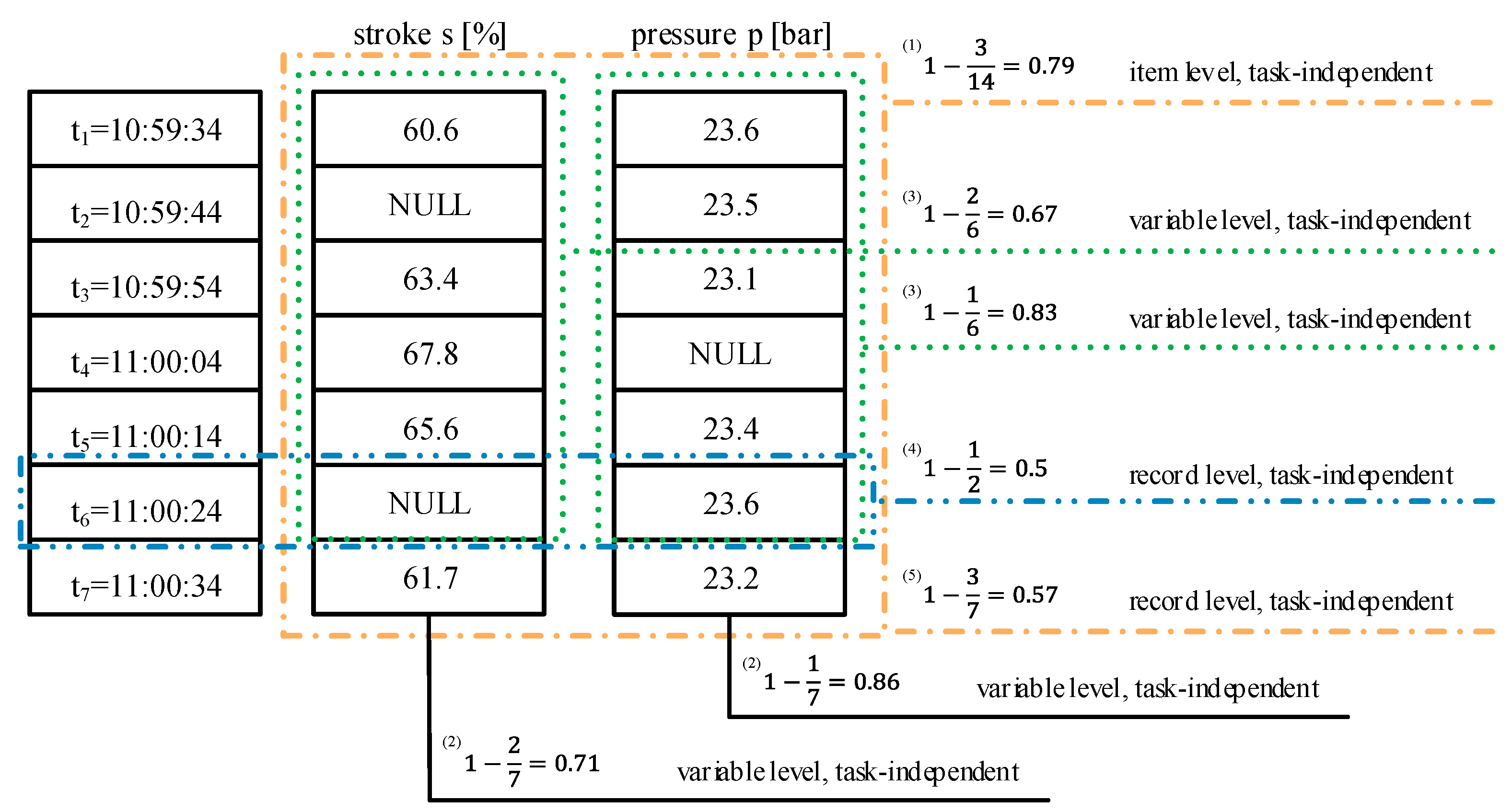
• Task-independent: Several authors introduced an attribute concerning the task-independent completeness on item level, e.g., Value Completeness [34] or Data Item Completeness [30]. Besides their different names, the calculation of the metric is the same. The number of empty items (null values) in a data set is divided by the whole sum of items in the data set [28,30,33,34,35]. Sporadic missing values of sensors caused by, e.g., unstable wireless connection or sensor device outages such as limited battery life or environmental interferences [40], impact this completeness. The example (1) in Figure 5 shows task-independent completeness on item level of $0.79$ (3 items out of 14 are NULL).
• Task-dependent: No attribute is introduced. One specific item is either existing or not. It is not reasonable to evaluate task-dependent completeness on single items.

Variable level:

• Task-independent: The task-independent attribute on variable level considers the empty items of one variable in relation to the number of available records [16,28,33,34,36,37]. The example (2) in Figure 5 illustrate this attribute which is called, among others, Column Completeness [16], Structural Completeness [36] or Attribute Completeness [37]. Even though several different names are introduced over time, the basic concept and the calculation is similar. However, Scannapieco and Batini 2004 further differentiate in a weak and a strong metric [34]. In contrast to the weak completeness (example (2) in Figure 5), the strong completeness is either 0 or 1 (0 for missing values in a variable and 1 for a complete variable). In Figure 5, the Strong Attribute Completeness is 0 for each variable. For sensor data, a window is defined, calculating the completeness value subsequently [38,39]. Based on a window of one minute, example (3) in Figure 5 reveals task-independent completeness on variable level of $0.67$ for stroke and $0.83$ for pressure in the first minute.
• Task-dependent: For this attribute, the expectations concerning the values or the amount of data are considered, respectively [16,28,34,36,37]. Most metrics observe whether all expected values of a variable are included in the data or not. If the valve’s stroke, which can vary from fully closed (stroke = 0%) to fully opened (stroke = 100%), only contains values between 60% and 90%, task-dependent completeness on variable level, e.g., Population Completeness [16] or Weak Relation Completeness [34], is reduced. The strong relation completeness [34] is 0 in this case. In contrast, the Content Completeness [36] refers to the precision of the data. If data does not contain as much information as required, e.g., only one decimal digit instead of the required three decimal digits, the completeness is reduced. Beside the metrics concerning the values of the variables, also metrics evaluating the amount of data of each variable is reasonable. The completeness concerning the amount of data is reduced if the valve’s stroke is gathered for 2 h even though the use case requires 3 h.

Record Level:

• Task-independent: Two different viewpoints are introduced for the record level. The first viewpoint considers and assess each record individually. This completeness is calculated based on the empty items in one record in relation to the number of variables. The record $t_6$ (example (4) in Figure 5) has a Weak Tuple Completeness [34] and Record Completeness [37] of $0.5$ since one of the two sensor signals is missing. The strong tuple completeness [34] evaluates the completeness of the record ${\mathrm{t}}_6$ as $0$, since it is not complete. The second viewpoint observes how many records with missing values are contained in the data set [37]. In Figure 5, the Empty Records in a Data File [37] is $0.57$ (5).
• Task-dependent: On record level, only one task-dependent attribute is introduced [37] concerning the amount of data rather than the content. The quotient of number of records within a data set and expected number of records describes the Data File Completeness [37]. Like the variable level, this completeness is reduced if the entire data set contains data of 2 h even though 3 h are required. A consideration regarding a metric to assess task-dependent completeness on record level concerning the content is not introduced yet. It is not evaluated if the records show all the combinations of values that are expected.

Schema level:

• Task-independent: No attribute is introduced since it is not reasonable. If the schema is complete and contains all the relevant variables, can only be evaluated based on the expectations of the use case.
• Task-dependent: This attribute is evaluated based on the comparison of available and expected variables. If the condition monitoring of control valves requires a sensor for vibration, a data set containing only stroke, pressure and pressure difference is not complete. Consequently, the Schema completeness [16] and Conceptual Data Model Completeness [37] is reduced. Furthermore, the Conceptual Data Model Attribute Completeness [37] considers the format of the variables. If vibration is measured with a vibration velocity transducer providing values in $\mathrm{mm}/\mathrm{s}$; however, the values of an accelerometer in $\mathrm{m}·{\mathrm{s}}^{-2}$ is required and the completeness is reduced.

These metrics cover a wide range of attributes for completeness. Besides the literature defining metrics for completeness, further research is performed using and evaluating the introduced metrics for sensor and actuator data. For example, Otalvora et al., 2016 [41] use task-independent record completeness to assess the data quality of sensor data from drilling rigs. However, on record level, the task-dependent attribute is limited to concerns regarding the amount of data. The content, in particular the combinations of variable values in the records, is not considered even though Wand and Wang 1996 [11] already observed that completeness is a question of “data combinations rather than just [...] null values” [11]. On variable level, it is observed whether all possible values are covered by the data. The stroke of control valves should contain values from fully closed (stroke = 0%) to fully opened (stroke = 100%).

However, none of the introduced completeness metrics is concerned whether the stroke values appear with different combinations of the other variables, e.g., pressure. The task-dependent completeness on record level still is a research gap. Closing the gap, this paper introduces the concept of data set completeness. Data set completeness examines the combinations of variables in a multi-dimensional data set of sensor and actuator data. The proposed metric for data set completeness indicates whether the data set is complete and balanced regarding the different combinations of variable values. The utilization of the feature space is described by the data set completeness.

The paper hypothesizes that the data set completeness metric and its visualization reveal the structure of a multi-dimensional data set in more detail than other commonly used statistics and visualizations in data preparation. Furthermore, it will be shown that a reduction of data set completeness harms model accuracy of data-driven models for condition-based maintenance. Thereby, model accuracy is measured by the coefficient of determination $R^2$ and the root mean squared error (RMSE) of the prediction model. The coefficient of determination (1) measures the variance of the model output that can be explained by the model. A high coefficient of determination indicates a good predictability of the model output based on the model input. The RMSE (2) measures the deviation of the predicted and the actual model output providing information about the precision of the model. Due to the impact on model accuracy, the importance of assessing data set completeness is revealed. The example of condition monitoring in control valves will show that a reduced metric for Record [37], Data File [37], Tuple [34] Completeness and Empty Records in a Data File [37] (cf. Table 1), which are the only metrics on record level in the related literature, and does not reduce the data set completeness and decrease the model accuracy necessarily. However, a reduced data set completeness will decrease model accuracy.

$$R^2=\frac{{\displaystyle \sum }{\left(y_i-{\widehat{y}}_i\right)}^2}{{\displaystyle \sum }{\left(y_i-{\overline{y}}_i\right)}^2}$$

(1)

$$RMSE=\sqrt{\frac{1}{n}{\displaystyle \sum }{\left({\widehat{y}}_i-y_i\right)}^2}$$

(2)

with ${\widehat{y}}_i=$ predicted output, $y_i=$ actual output, ${\overline{y}}_i=$ mean of actual output and $n=$ number of observations.

To develop an efficient metric for data set completeness, four requirements have to be fulfilled [42]. First, the metric requires a defined minimum and maximum value (R1). For data quality, the common definitions set the minimum to 0—perfectly poor data quality—and the maximum to 1—perfectly good data quality. Furthermore, the metric should be interval-scaled (R2), enabling the interpretation of intervals, e.g., completeness of 0.2 is half as complete as completeness of 0.4. Third, the use and the calculation of the metric should be independent of hyper-parameters (R3) to receive an objective measure. It is essential that two different users of the metric obtain the same numerical result. Last, an appropriate aggregation (R4) is required to include the metric in high-level key indicators for data quality. A fifth requirement, economic efficiency, is not considered in this paper.

For a visualization, requirements concerning the usability should be considered. However, this paper leaves the evaluation of the visualization for future work, due to the greater extent. In this paper, the visualization is used to support the plausibility check of the proposed metric.

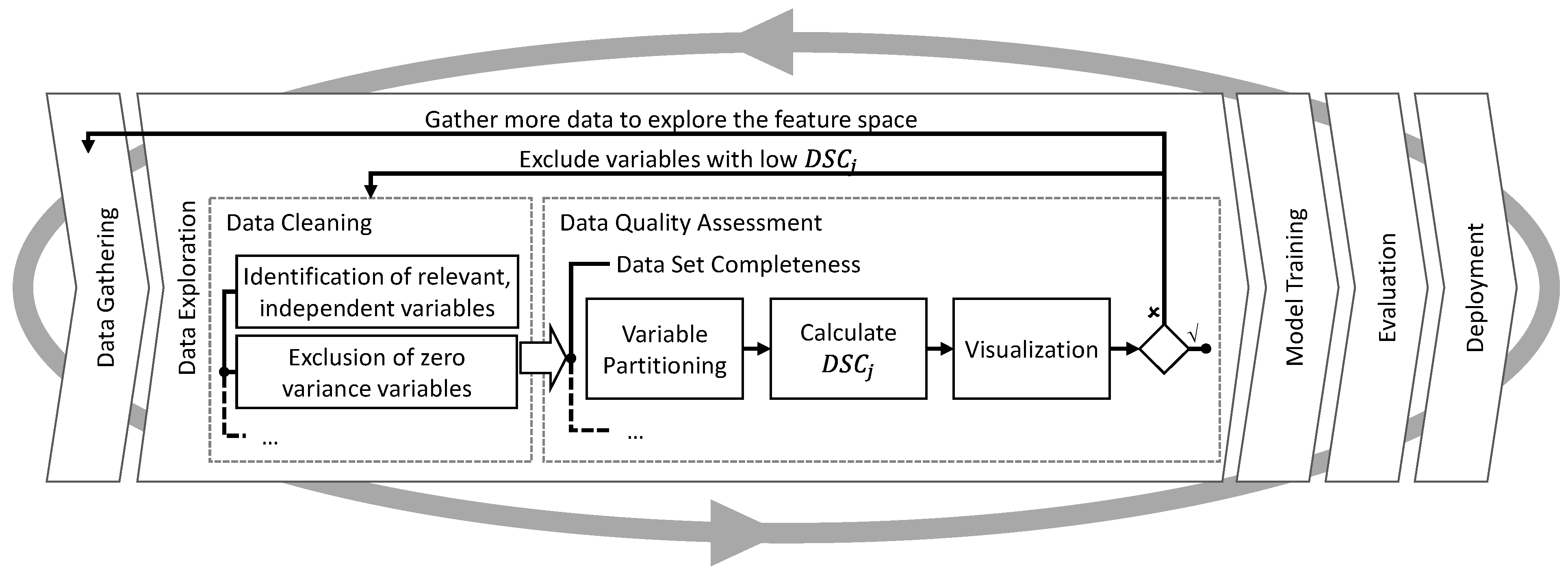
4. The Concept for the Assessment of Data Set Completeness

The following paragraphs propose a metric and a visualization to assess data set completeness in multi-dimensional data sets of sensor and actuator data.

The multi-dimensional data set $I$ includes $n$ variables (3) and each of these variables ${\overrightarrow{X}}_i$ consists of $m$ expected observations (4) (see also

Table 2. Nomenclature for the concept of data set completeness.

Parameters
$\overrightarrow{I}$	$\mathrm{Data}\mathrm{set}\mathrm{including}n$ variables	$K_j$	$\mathrm{Number}\mathrm{of}\sec \mathrm{tions}\mathrm{of}\mathrm{class}j$
$n$	Number of variables	${\mu }_j$	$\mathrm{Number}\mathrm{of}\mathrm{minority}\sec \mathrm{tions}\mathrm{in}\mathrm{class}j$
${\overrightarrow{X}}_i$	$\mathrm{Variable}i$$\mathrm{including}m$ observations	$DS{C}_j$	$\mathrm{Data}\mathrm{set}\mathrm{completeness}\mathrm{of}\mathrm{class}j$
$m$	Number of observations	$S{V}_j$	$\mathrm{Sec}\mathrm{tion}\mathrm{volume}\mathrm{of}\mathrm{class}j$
$d$	Distance of two vectors	$S{B}_j$	$\mathrm{Sec}\mathrm{tion}\mathrm{balance}\mathrm{of}\mathrm{class}j$
$\eta$	Number of observations in one section	$Min$	Minimum value
${\overrightarrow{v}}_j$	$\mathrm{Class}\mathrm{vector}\mathrm{of}\mathrm{class}j$	$Max$	Maximum value
$\overrightarrow{s}$	Variable vector	$Mean$	Mean value
${\overrightarrow{e}}_j$	$\mathrm{Equally}\mathrm{distributed}\mathrm{class}\mathrm{vector}\mathrm{of}\mathrm{class}j$	$SD$	Standard deviation
${\overrightarrow{\omega }}_j$	$\mathrm{Worst}\mathrm{distributed}\mathrm{class}\mathrm{vector}\mathrm{of}\mathrm{class}j$	$RSD$	Relative standard deviation (SD/Mean)
$K$	Number of sections	$IQR$	Interquartile range (3rd quartile–1st quartile)
$k_i$	$\mathrm{Number}\mathrm{of}\mathrm{classes}\mathrm{of}\mathrm{variable}i$
	Variables	Indices
$q$	Flow	$i$	Variable
$s$	Stroke	$j$	Class
$p$	Pressure upstream (before the valve)
$\Delta p$	Pressure difference before and after the valve
$p_s$	Signal pressure
Terms
variable	A variable represents one sensor or actuator of an aPS. The values of a variable are numerical, either continuous or discrete.
class	A class describes a specific value interval of a variable. Classes do not overlap but border to each other and cover the whole value range of a variable.
section	A section represents an area of the n-dimensional feature space described by the respective classes of the n variables. A section is an n-dimensional bin of the feature space.
feature space	The feature space is the n-dimensional space, which is created between the variables.

Nomenclature p. 16).

$$I=\left[{\overrightarrow{X}}_1,\dots ,{\overrightarrow{X}}_n\right]$$

(3)

$${\overrightarrow{X}}_i=\left[\begin{array}{c}{x}_{i_1}\\ \dots \\ x_{i_m}\end{array}\right]$$

(4)

The variables ${\overrightarrow{X}}_i$ represent sensor or actuator data along the time axis $t_1\dots t_m$ of an aPS. The values $x_{i_1}\dots x_{i_m}$ are numerical values, continuous or discrete. For condition monitoring of control valves, the variables stroke $s$, pressure $p$ and pressure difference $\mathsf{\Delta }p$ are considered.

4.1. Assumptions and Prerequisites

Carefully performed data preparation is required before the assessment of data set completeness. This includes identifying relevant data, the data gathering and integration as well as the assessment of other data quality dimensions. It is assumed that possible data quality defects of other data quality dimensions are rectified. Missing synchronicity of sensor and actuator data, for example, leads to a misfit of the time reference. While the observation of one sensor is recorded at time $t$, the observation of another sensor is recorded at time $t+1$. In this case, it is not possible to bring both sensors into relation. This needs to be solved before the assessment of data set completeness. Furthermore, it is assumed that the data set includes all relevant variables required to solve the task at hand, meaning high Schema Completeness [16] is given. Also, the variables of this data set are supposed to be independent and high utilization of the feature space is expected. For dependent sensor data, e.g., the positively correlated stroke $s$ and the signal pressure of a control valve $p_s$, a fully utilized features space is not possible since a high signal pressure causes a high stroke. Data with high signal pressure and low stroke is unfeasible and not represented in the data set. Based on these assumptions and prerequisites, the data set completeness can be assessed using the following metric.

4.2. Metric for Data Set Completeness

For data set completeness, the presence and balance of the value combinations for the variables ${\overrightarrow{X}}_i$ in $\overrightarrow{I}$ are evaluated. High data set completeness is given when observations of the data set equally utilize the feature space. In a three-dimensional case, the utilization of the feature space is easily assessed by a graphical representation. However, such representations are limited in the number of dimensions. Assessing the data set completeness numerically requires a metric to quantify the presence and balance of the value combinations.

To reduce computational complexity, the feature space is partitioned into different sections (cf. Figure 6a). A section is an n-dimensional bin in the feature space. These sections are observed for data set completeness rather than the single values with arbitrary precision. All sections are defined by a specific value interval of each variable. In the example of Figure 6a, observations with a stroke between $75\%$ and $80\%$, a pressure between $17.5$ and $18.5$ bar and a pressure difference between $0.0$ and $3.0$ bar belong to one section (marked as Box_example in Figure 6a).

To identify the value intervals of the variables—so-called classes—each variable is partitioned individually into $k_i$ classes. The classes do not overlap but border to each other, representing one specific value interval. A superscript, e.g., $j^l$ and $j^u$ for class $j$, denotes the lower and upper bound of each class, respectively. The lower bound of the first class represents the minimum value, whereas the upper bound of the last class represents the maximum value of the variable. Different approaches can be chosen to partition the values range of the variables. First, the partitioning of each variable can be performed based on simple rules derived from histograms. The optimal width of the classes can be calculated by quotients, based on the number of observations, e.g., Sturges-rule [43], or in combination with the spread of the data, e.g., Freedman–Diaconis rule [44]. In this case, the classes are of equal width. This might not get along with the characteristics of the data.

Two different operational points (e.g., Figure 1a) should be in two different classes to be examined for their combinations with the other variables individually. On the other side, one operating point should not be split into two classes unnecessarily. This is not ensured when using Sturges or Freedman–Diaconis-rule. A second approach, the one-dimensional clustering such as Jenks Natural Breaks [45], partitions the variable into classes with different widths based on the data’s characteristics. The clustering takes into account the potential operating points. While the clustering splits the operating points to separate classes, the Sturges rule and Freedman–Diaconis rule might split one operating point or mix several points together due to the fixed width of the classes. A third approach, avoiding wrong breaks of the value range, performs the partitioning based on expert knowledge. The expert can take specific requirements set by the use case into account. In the following, it is assumed that the experts define the classes of the variables. For future work, the implementation of a one-dimensional clustering is considered, automating the process.

Splitting the n-dimensional feature space into its sections based on the classes results in the total number of $K$ (Equation (5)). An example for this parameter and the following is given in the grey box of Figure 6 to increase clarity.

$$K={\displaystyle \prod }_{i=1}^n{k}_i$$

(5)

All observations $m$ of the data set $I$ are assigned to their respective section according to the values of the variables ${\overrightarrow{X}}_i$. The number of observations $\eta$ within one section is considered as a feature for the calculation of the data set completeness. To evaluate the completeness and balance of the sections, each dimension of the feature space, meaning each variable is considered individually. The class vector ${\overrightarrow{v}}_j$ (6) represents the number of observations $\eta$ of the different sections that belong to one specific class $j$ of the considered variable $i$ (in order to preserve greater clarity, ${\overrightarrow{v}}_j$ and all further parameters are written without the index $i$). Based on this class vector, the balance of one slice of the feature space can be assessed (cf. class 2 of variable $X_3$ in Figure 6a, highlighted in blue). In order to consider the distribution of observations between the classes of one variable $i$, the variable vector $\overrightarrow{s}$ is introduced additionally (7). The variable vector $\overrightarrow{s}$ represents the sum of observations in each class $j$ of variable $i$. Based on these two vectors, each dimension is assessed individually: once across the dimension via the class vector and once along the dimension via the variable vector. Figure 6c,d visualize the class and variable vectors for dimension $X_1$ and $X_2$, respectively.

$$\begin{array}{cc}\begin{array}{c}{\overrightarrow{v}}_j=\left[{\eta }_1,\dots ,{\eta }_{K_j}\right]\\ \mathrm{with}{\mathrm{K}}_j=\frac{K}{k_i}\end{array}& \hspace{1em}\hspace{1em}\hspace{1em}\hspace{1em}\forall i=\left[1\dots n\right]\end{array}$$

(6)

$$\overrightarrow{s}=\left[{\displaystyle \sum }{\overrightarrow{v}}_1,\dots ,{\displaystyle \sum }{\overrightarrow{v}}_{k_i}\right]\hspace{1em}\hspace{1em}\hspace{1em}\hspace{1em}\hspace{1em}\forall i=\left[1\dots n\right]$$

(7)

The data set completeness $DS{C}_j$ of each class $j$ (8) consists of two aspects: first, the balance of the class vector ${\overrightarrow{v}}_j$, called section balance $S{B}_j$, and second, the relative number of observations in the considered class, called class volume $C{V}_j$. While the section balance $S{B}_j$ evaluates the balance of the available observations within one class, the class volume $C{V}_j$ evaluates the relative number of observations in the considered class compared to the other classes of variable $i$ ($\overrightarrow{s}$). A perfect data set completeness is characterized by a perfectly balanced distribution of observations around the sections within one class and perfectly equally distributed observations around the classes. In this case, the feature space is equally utilized.

$$\begin{array}{ll}DS{C}_j=\alpha ·S{B}_j+\left(1-\alpha \right)·C{V}_j& \begin{array}{c}\hspace{1em}\hspace{1em}\hspace{1em}\forall j=\left[1\dots k_i\right]\\ \hspace{1em}\hspace{1em}\hspace{1em}\forall i=\left[1\dots n\right]\end{array}\end{array}$$

(8)

The constant factor $\alpha$ defines the importance of the two aspects. If $\alpha <0.5$, it is more important that the class contains a higher relative number of observations rather than the sections being balanced. This could be a reasonable approach when resampling the data to balance the data set is an appropriate preprocessing step for the use case at hand. A default $\alpha =0.5$ is proposed, given the section balance $S{B}_j$ and the class volume $C{V}_j$ equal importance.

The metric for the section balance $S{B}_j$ measures the balance of observations around the sections of one class. In the best case, each section contains an equal number of observations. The metric is derived by the imbalance degree of Ortigosa-Hernández et al. 2017 [46]. In contrast to other imbalance measures such as imbalanced ratio (amount of data in the smallest section divided by the amount of data in the biggest section) the imbalance degree takes into account the distribution of all sections and not only the smallest and biggest. In order to do so, the distance $d$ between the class vector ${\overrightarrow{v}}_j$ and the equally distributed vector ${\overrightarrow{e}}_j$ is calculated as measure for the imbalance. The higher the distance to the equally distributed vector, the higher the imbalance of vector ${\overrightarrow{v}}_j$. The distance $d$ of the two vectors is calculated based on the total variation distance (9). Thereby, the equally distributed vector ${\overrightarrow{e}}_j$ consists of the same number of sections, contains the same number of observations (${\displaystyle \sum }\eta$), but shows an equal distribution of these observations.

$$\begin{array}{ll}\mathrm{d}\left({\overrightarrow{v}}_j,{\overrightarrow{e}}_j\right)=0.5{\displaystyle {\displaystyle \sum }_{z=1}^{K_j}}\left|{\overrightarrow{v}}_j{}_z-{\overrightarrow{e}}_j{}_z\right|& \begin{array}{c}\hspace{1em}\hspace{1em}\hspace{1em}\forall j=\left[1\dots k_i\right]\\ \hspace{1em}\hspace{1em}\hspace{1em}\forall i=\left[1\dots n\right]\end{array}\end{array}$$

(9)

In order to make the distance $\mathrm{d}\left({\overrightarrow{v}}_j,{\overrightarrow{e}}_j\right)$ interpretable and comparable, it is normalized to a range between 0 and 1. In order to do so, the distance measure is divided by the distance between the equally distributed vector ${\overrightarrow{e}}_j$ and the worst distributed class vector ${\overrightarrow{\omega }}_j$. The quotient then expresses the degree of imbalance in percentage. This worst distributed class vector ${\overrightarrow{\omega }}_j$ complies with the following requirements: ${\overrightarrow{\omega }}_j$ contains the same number of observations as ${\overrightarrow{v}}_j$; minority sections of ${\overrightarrow{v}}_j$ $({\overrightarrow{v}}_j{}_z<{\overrightarrow{e}}_j{}_z)$ are set to 0; majority sections of ${\overrightarrow{v}}_j$ $({\overrightarrow{v}}_j{}_z>{\overrightarrow{e}}_j{}_z)$ are set to ${\overrightarrow{e}}_j{}_z$ except for one section containing all remaining observations. Furthermore, the resulting quotient is multiplied by a correction factor taking into account the size of the vector and the number of minority sections within the vector. Otherwise the vector ${\overrightarrow{v}}_A={\overrightarrow{\omega }}_A=\left[20, 0\right]$ receives the same imbalance score as vector ${\overrightarrow{v}}_B={\overrightarrow{\omega }}_B=\left[20, 10, 10, 0\right]$, since both are maximal imbalanced for a number of minority sections of 1. However, a vector with less minority sections in relation to the total number of sections, e.g., ${\overrightarrow{v}}_B$, is less imbalanced than a vector with more minority sections, e.g., ${\overrightarrow{v}}_A$. Therefore, the imbalance metric is multiplied by the quotient of the number of minority sections ${\mu }_j$ and the maximum of potential minority sections $K_j-1$. This quotient achieves the maximum of 1, when all sections except for one are minority sections. The minimum of 0 is achieved when zero minority sections are observed which is only the case if the vector ${\overrightarrow{v}}_j$ equals ${\overrightarrow{e}}_j$. In this way, vector ${\overrightarrow{v}}_A$ reveals an imbalance degree of 1 while vector ${\overrightarrow{v}}_B$ reveals an imbalance degree of $0.33$.

The final section balance $S{B}_j$ of class $j$ equals 1 minus the derived imbalance degree (10). Since the quotient of the two distances $d$ is between 0 and 1, and the correction factor is also between 0 and 1, the imbalance degree as well as the section balance $S{B}_j$ achieves maximal 1 for perfectly good data quality and minimal 0 for perfectly poor data quality.

$$\begin{array}{ll}S{B}_j=1-\left(\frac{\mathrm{d}\left({\overrightarrow{v}}_j,{\overrightarrow{e}}_j\right)}{\mathrm{d}\left({\overrightarrow{\omega }}_j,{\overrightarrow{e}}_j\right)}·\frac{{\mu }_j}{K_j-1}\right)& \begin{array}{c}\hspace{1em}\hspace{1em}\hspace{1em}\forall j=\left[1\dots k_i\right]\\ \hspace{1em}\hspace{1em}\hspace{1em}\forall i=\left[1\dots n\right]\end{array}\end{array}$$

(10)

The metric for the class volume $C{V}_j$ compares the number of observations of class j with the number of observations of the other classes of variable $i$ ($\overrightarrow{s}$). In the best case, all classes contain the same number of observations leading to a balanced distribution across the variable $i$. In order to evaluate the number of observations ${\displaystyle \sum }{\overrightarrow{v}}_1$, it is divided by the maximum of observations in one class of variable $i$ (11). For a perfectly balanced variable, e.g., $\overrightarrow{s}=\left[10, 10, 10, 10\right]$ the class volume $C{V}_j$ equals 1 for each class. For a perfectly unbalanced variable, e.g., $\overrightarrow{s}=\left[40, 0, 0, 0\right]$ the class volume $C{V}_j$ for the first class equals 1, while all other classes achieve a class volume $C{V}_j$ of 0. This ensures, that the metric for class volume is between 0 and 1, indicating perfectly poor and perfectly good data quality.

$$\begin{array}{ll}C{V}_j=\frac{{\displaystyle \sum }{\overrightarrow{v}}_1}{\max \left(\overrightarrow{s}\right)}& \begin{array}{c}\hspace{1em}\hspace{1em}\hspace{1em}\forall j=\left[1\dots k_i\right]\\ \hspace{1em}\hspace{1em}\hspace{1em}\forall i=\left[1\dots n\right]\end{array}\end{array}$$

(11)

The section balance $S{B}_j$ as well as the class volume $C{V}_j$ achieve values between 0 and 1. Consequently, the data set completeness $DS{C}_j$ (8) take on values between 0 and 1. Perfectly good data quality in terms of data set completeness is achieved when the classes of the variables show an equal number of observations and these observations are balanced around the different sections of each class. In this case, the metric for data set completeness is valued 1.

4.3. Visualization of the Data Set Completeness

The proposed metric for the data set completeness $DS{C}_j$ provides values for each class $j$ of the variable $i$. In a big data set with several variables and classes, an evaluation based on the numeric values for $DS{C}_j$ is not easily accessible for an expert. Therefore, a visualization is required to represent the results clearly and intuitively. A heat map is proposed, coding the data set completeness of each class in a color bar. In this way, the expert can easily access and identify classes with insufficient data set completeness. An abstracted example showing the structure of the visualization is given in Figure 7. Each variable is represented by one bar. The bottom and the top of the bar mark the minimum and the maximum value of this variable, respectively. The border of the variable classes segments the bar. Each segment is colorized based on the value for data set completeness of the respective class. The color bar on the right edge of the visualization informs about the interpretation of the colors. The color bar is fixed with a minimum of $0$ and a maximum of $1,$ representing perfectly poor and perfectly good data quality in terms of data set completeness. In order to enable the iterative assessment of the data set completeness, the visualization is implemented as a graphical user interface in Python 3.7 prototypically. Based on the package ‘dash’ (version 1.18.1), a web-based interface is created given the expert the possibility to select and deselect variables of a drop-down menu. The recalculation based on the variable choice is triggered automatically, updating the heat map of the data set completeness.

The data set completeness is highly dependent on the composition of the data set. Adding or excluding variables changes the dimensionality of the feature space and the data set completeness for every single class. Therefore, assessing data set completeness and identifying the appropriate composition of variables is an iterative task. Since each variable requires an own bar, the use of the metric and visualization for data set completeness is limited by the width of the plot. Furthermore, the dependency of the metric’s value on the dimensionality of the feature space raises issues regarding the curse of dimensionality [47], particularly the trend of the metric values to equalize each other. In order to preserve clarity and prevent the curse of dimensionality, the number of variables restricts the applicability. However, in model-based data-driven condition monitoring, expert knowledge and data are combined to solve the task. This is not reasonable in systems with several hundred variables or more. In those cases, massive amounts of data are required to extract information with artificial intelligence methods rather than model the dependencies based on the experts’ input. Use cases of smaller systems with the problem of limited amounts of data are the focus of this work. In this case, model-based data-driven condition monitoring is reasonable and a multi-dimensional but not high dimensional feature is expected.

The workflow in Figure 8 shows the assessment of the data set completeness in the context of a data mining process. In the data cleaning process, the prerequisites (cf. Section 4.1) are created. The relevant, independent variables for the task at hand need to be identified and variables with zero variance should be excluded. Subsequent to the data cleaning, the partitioning of the variables is performed. The expert needs to identify the operating points to partition the variables appropriately. Based on this, the data set completeness of each class of the variables is calculated and visualized. The expert iteratively prepares a data set with high data quality by gathering more data or by excluding variables with low data set completeness. Finally, a well-prepared data set with high data set completeness can be used to train a data-driven model.

5. Application and Discussion of the Proposed Metric and Visualization

The proposed metric is evaluated based on the use case of condition monitoring of control valves. In this paper, a model-based data-driven approach is chosen. Expert knowledge is used to identify a valve’s relevant input and output parameters (model-based) and data is used to train the dependencies between these parameters (data-driven). In this way, available expert knowledge is utilized, but detailed physical modeling involving fluid mechanics is avoided. In literature, also other approaches are proposed. Signal-based approaches, for example, observe the characteristics of individual signals to detect deviation of normal behavior. Leakage of valves is a common problem that is detected based on the characteristics of the acoustic [48,49,50] or pressure [51] signal. However, the system dynamics are not considered in signal-based approaches, making them vulnerable to regular changes and movements, raising false alarms. Also, classification algorithms are used, which require a labeled training data set, including fault-free and faulty data. Several signals and combinations of signals serve to identify the patterns, which separate fault-free and faulty data. Acoustic and vibration data [52,53,54] or parameters such as pressure, temperature and stroke [55] provide features for classification. Furthermore, novelty detection algorithms are applied to identify changes in valve behavior. Neural networks are the most common algorithms for novelty detection [56,57]. Besides, also one-class support vector machines are applied [58]. These methods cause high computational costs for the identification of the best hyper-parameters.

In contrast, model-based data-driven approaches reduce complexity in the training process due to the input of experts regarding the input and output parameters and their relevant features. Therefore, this approach is promising for a broad application in the industry. The approach in this paper aims at predicting the flow of the valve $q$ considering the valve’s stroke $s$, pressure $p$ as well as the pressure difference $\Delta p$ as input variables [2]. The residuals of the predicted and the actual flow serve as a feature for anomaly detection. High residuals reveal a change of the dependencies between the variables and indicate an anomaly. The relevance of the variables stroke, pressure and pressure difference is explained easily: a higher stroke increases the cross-section of the valve and a higher flow can pass the valve. Analogous to this, a higher pressure or pressure difference leads to a higher flow. A data-driven model trains these dependencies to predict the flow $q$ of the valve given the values for stroke $s$, pressure $p$ and pressure difference $\Delta p$.

The available data set was gathered at test runs. Experts designed a procedure that covers a wide range of the scope of function for the considered control valve. This enables data-driven models to learn the valve behavior. The test run was repeated 10 times to include the normal volatility of the data in the data-driven model. In total, $27,000$ observations with a sampling rate of $0.5$ s were considered in the following. It was expected that the completeness of the data set is high. For reasons of anonymization, the variables are normalized between 0 and 1. A train-test-split was performed, isolating 30% of the data for test purposes.

Prior to evaluating the proposed metric and visualization for data set completeness, the descriptive statistics of the training data set are discussed. The stroke $s$ is equally distributed between the minimum and maximum (cf. Figure 9). The distribution shows a mean of $0.50$ and a standard deviation of $0.29$. The pressure $p$ and the pressure difference $\Delta p$ clearly indicate four different operating points, which were caused by the design of the test runs (cf. histograms of Figure 9). The pressure $p$ shows a higher number of observations for higher values. The boxplot marks lower values of $p$ $(0<p<0.25)$ as outliers, since these values are rare. A high data set completeness requires equally distributed data around the whole feature space. E.g., high pressure $p$ should occur with high as well as low stroke $s$ and the other way around. Furthermore, a high-pressure difference $\Delta p$ should be observed for high upstream pressure $p$ as well as for low upstream pressure $p$ and the other way around.

To assess the data set completeness of this training data, each variable is partitioned into four classes, representing the operating points. The variable stroke $s$ could also be partitioned into more classes, since no clear operating points are identifiable.

The data set completeness (cf. Figure 10) shows high values for stroke and pressure difference, while the data set completeness decreases for lower values of pressure. Two aspects cause the low data set completeness for lower pressure. First, the absolute number of observations is low for a pressure between 0 and 0.25 (cf. Figure 9). Less than 1000 observations are observed for a single bar of the histogram, while a pressure between 0.75 and 1 shows frequencies of more than 5000 observations. This affects the class volume $C{V}_j$, decreasing the data set completeness. Second, low pressure does not allow a high-pressure difference. For that reason, the sections of low-pressure and high-pressure difference of the feature space do not contain observations, which decrease the section balance $S{B}_j$ and data set completeness in these classes, respectively.

However, such physical constraints do not harm the quality of the data. Only the unbalanced distribution of the data for lower and higher pressure (class volume $C{V}_j$) is unfavorable. This is why the expert is still required. The results need to be interpreted appropriately. Even though the data set completeness is minimal for low pressure, the data set still is useful. On average, stroke and pressure difference achieve a data set completeness of 0.79. In contrast, pressure achieves a mean data set completeness of 0.51.

If only stroke and pressure difference are considered, the data set completeness reveals a very high utilization of the feature space (cf. Figure 11a). For this two-dimensional consideration, the metric results for data set completeness can be verified based on a simple scatter plot (cf. Figure 11b) visualizing the observations between the two variables. Each section of the feature space contains several observations, given a reasonable basis to train a valid model to predict the valve’s flow.

To model the dependencies between flow $q$, stroke $s$, pressure $p$ and pressure difference $\Delta p$, a random forest regression was trained using the flow as the dependent and the stroke, pressure and pressure difference as the independent variable. The resulting model represents the benchmark for evaluating the proposed metric and visualization for data set completeness.

The model was trained in Python 3.7 with the random forest regressor of the scikit-learn package (version 0.23.1). A random search was performed, changing the number of generated decision trees, the minimum number of samples in one leaf and the tree’s maximum depth. The evaluation was performed based on the coefficient of determination, RMSE and the computation time required to use the model. In this way, the random forest regressor is pruned, reducing the computational complexity while keeping the accuracy of the model at a maximum. Three-fold cross-validation was performed to receive validated results.

The results show that a random forest regression with a low number of decision trees achieves high coefficients of determination ($R^2>0.98)$. Due to the conditions during the test runs, noise and other disturbances, such as environmental influences are eliminated. Therefore, the data easily reveals the dependencies of the variables. A deeper look at the trade-off of precision (low RMSE) and computation time (low mean-score time) suggests a random forest with 5 trees, a minimum number of 5 samples in one leaf and a maximum depth of 50 (cf. Figure 12). The Pareto front is a matter of subjective perception (cf. Figure 12 gray lines). Another hyper-parameter combination achieving a lower RMSE based on a higher computation time could also be reasonable. This work will not emphasize this since it is not valuable for the discussion of the hypotheses.

The trained random forest regression model receives a mean coefficient of determination of 0.99989. This means the model covers almost the whole variance in the training data set. The mean RMSE of $0.00268$ in the test data confirms the validity of the model. The prediction of the flow is exact and deviates from the actual flow value only by $\mp 0.00268$. The feature importance of 0.926 for stroke, 0.001 for pressure and 0.073 for pressure difference show that stroke has the highest impact on the flow by far. This is a reasonable result. A higher stroke increases the flow cross-section, thus influencing the flow significantly. The pressure difference further influences the flow. While keeping the stroke constant, the increase of the pressure difference leads to a higher flow. Pressure $p$ does not have much influence on the model.

In order to prove the hypothesis, the available training data is manipulated. First, 25% of the training data is randomly deleted (data set A). Consequently, the record completeness is reduced to 75%, while the data set completeness stays constant since the data is deleted randomly without changing the structure of the data. It is expected that the metric and visualization of data set completeness and the accuracy of the prediction model trained based on data set A is similar to the original data set. Second, 25% of the training data is deleted in selected distinct sections of the feature space, deteriorating the data structure (data set B). It is expected that the metric and visualization of data set completeness detect the data quality deficiency by a reduced metric value and that the modal accuracy decreases. The following section discusses the descriptive statistics of the different data sets to analyze the structure in more detail.

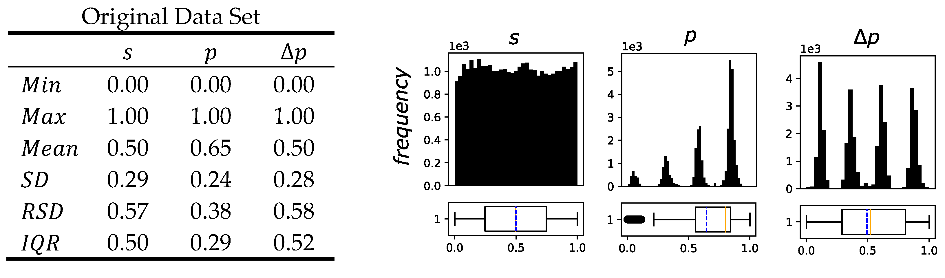
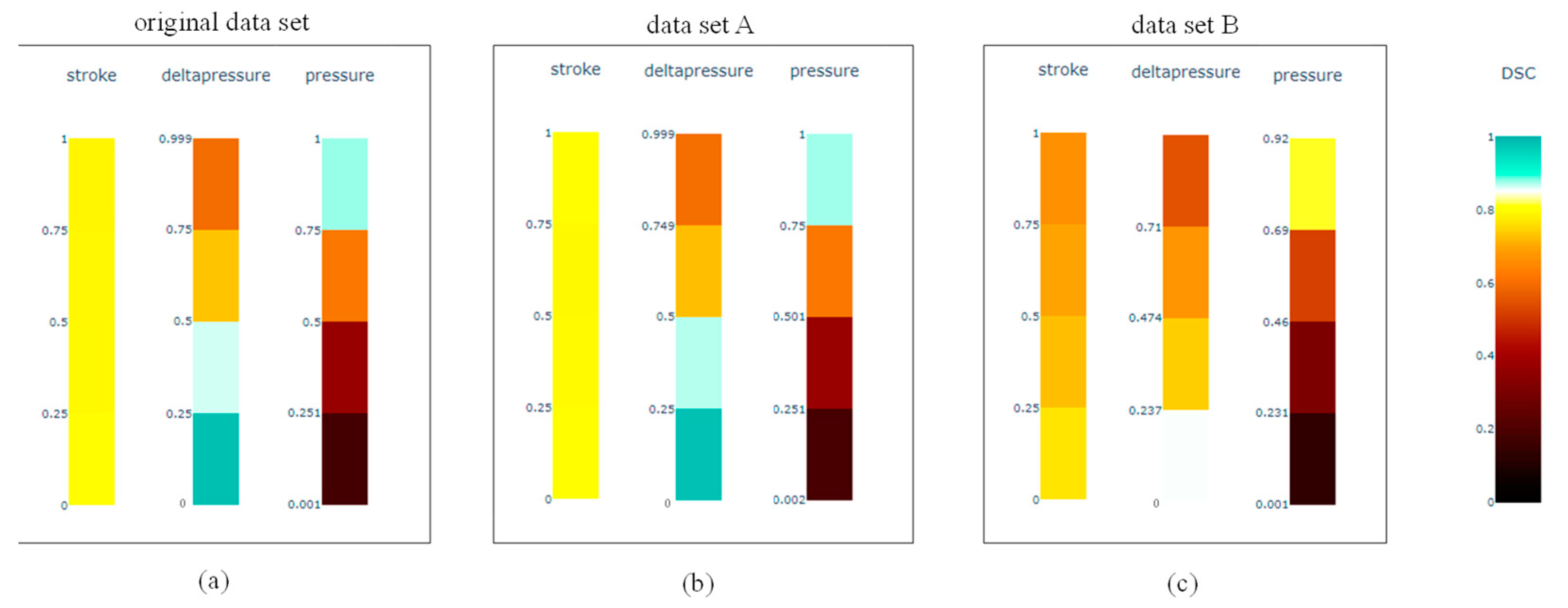
5.1. Comparison of the Different Data Sets

The original data set and the manipulated data sets A and B are compared to demonstrate the weakness of common metrics and visualizations of data in detecting the utilization of the feature space. The descriptive statistics and the histograms and boxplots of the different data sets are shown in Figure 13 The major difference between the original data set and the manipulated data sets is the absolute number of observations (cf. Figure 13 histograms). The original data set contains frequencies of the stroke up to $1000$, while the frequencies of the manipulated data sets are reduced to around $800$. However, the structure is unchanged. The histograms of pressure and pressure difference of data set A and B display the four different operating points unaffected. The descriptive statistics show a maximum pressure and pressure difference of 0.92 and 0.95 for data set B (cf. Figure 13 marked cells). This shows that some values in the upper range of the variables are no longer included in the data set. Furthermore, the interquartile range of the pressure difference in data set B is reduced significantly. The missing observations for higher values cause this. For pressure, a reduced interquartile range is not detected due to the still right-skewed distribution. Despite a reduced number of observations and the absence of a small value range in pressure and pressure difference, the common visualizations do not indicate major changes in the data sets structure.

The state-of-the-art metrics (cf. Table 1 on page 8) cannot reveal the differences in data set A and B either. An excerpt of the data set B is given in Figure 14, illustrating the numbers. Since 25% of the observations are deleted in both data sets, the Record Completeness [37] and the Weak Tuple Completeness [34] is $75\%$ for both data sets and the Empty Records in a Data File [37] are 25%, respectively (record level task-independent). In total, 6750 records out of 27,000 are missing. The Strong Tuple Completeness [34] equals 0 for both data sets since one missing record already reduces this metric to 0. Other task-independent metrics concerning the item and variable level are also similar in data set A and B. The completeness on item level is also 75%. In total, 20,250 items out of 81,000 are NULL values. The completeness on variable level is 75% for each variable and the Strong Attribute Completeness [34] is 0 for each variable since each variable includes at least one NULL value. For the task-dependent metrics, only the Data Value Completeness [37] is different in data set A and B. Since data set B is missing values for pressure higher than 0.92 and pressure difference higher than 0.95, the Data Value Completeness is reduced slightly. This was already detected by the descriptive statistics (cf. Figure 13). The completeness regarding the schema is unchanged compared to the original data set. All relevant variables are available.

In conclusion, the state-of-the-art statistics and metrics cannot detect structural differences in data set A and B, which could influence model training and model accuracy.

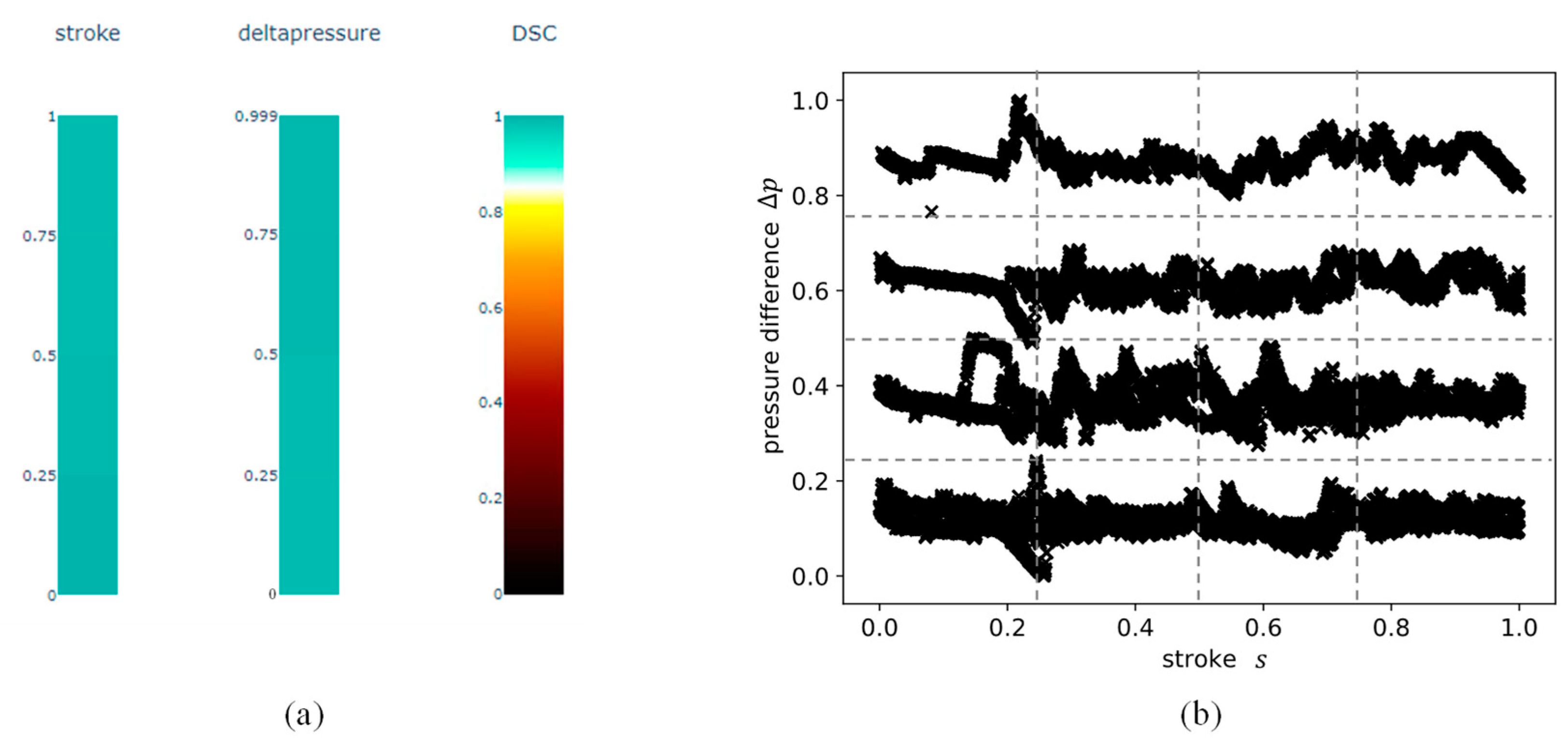
5.2. Application and Comparison of the Data Set Completeness Metric and Visualization of the Different Data Sets

In contrast to the metrics and visualizations in Section 4.1, the proposed data set completeness reveals the changes in the data set’s structure in data set B (cf. Figure 15). While the random deletion of observations in data set A does not change the utilization of the features space, the manipulation in data set B causes significant changes. Most classes show a reduced data set completeness (cf. Figure 15c). For stroke, the data set completeness decreases further with higher values. On average, stroke and pressure difference in data set B achieve a data set completeness of 0.71 and 0.70, respectively. This is a reduction by 0.08 and 0.09 percentage points compared to the original data set and data set A. The mean data set completeness for pressure in data set B is 0.44, which is 0.07 percentage points less than the original data set and data set A.

In order to check the metric and the visualization for plausibility, the data sets are examined further based on selected aspects. Since stroke and pressure difference are the variables with influence on flow, a more in-depth look is taken based on two-dimensional scatter plots. The scatter plots visualize the observations of the data set within the two variables (cf. Figure 16). The original data set contains observations in each section of the two-dimensional feature space. High utilization is observed. Data set A has a reduced record completeness. These missing data are distributed randomly around the whole feature space (cf. Figure 16 green box) and the utilization of the feature space is not affected. Data set B is missing four sections, leaving white spots on the feature space (cf. Figure 16 red boxes). Utilization is limited. However, the descriptive statistics do not indicate a change in the data set structure. In contrast, the data set completeness reflects this change by a reduced metric for almost all classes.

5.3. Results of the Random forest Regression of the Different Data Sets

The hypothesis implies that the accuracy of data-driven models decreases with decreasing data set completeness. However, reduced record completeness does not necessarily lead to losses in accuracy. In order to evaluate this, a random forest regression model is trained to data set A and B individually, comparing the coefficient of determination and the RMSE to the original data set (cf.

Table 3. Coefficient of determination and RMSE of the random forest regression of the original data set, data set A and B.

	Original	Data Set A	Data Set B
$R^2$	0.999	0.999	0.970
$RMSE$	0.00268	0.00283	0.04520

).

The random forest regression trained on data set B achieves a coefficient of determination of 0.97. This is a significant loss compared to the original data set. Furthermore, the RMSE increases to 0.045, indicating a loss in accuracy. The prediction of the random forest regression is not as precise as before. The original data set can represent the dependencies of flow, stroke, pressure and pressure difference accurately. However, the reduced data set completeness conceals parts of the dependencies causing losses in prediction accuracy.

In contrast, data set A achieves an accuracy similar to the original data set. This demonstrates that a reduced record completeness to 75% does not influence the accuracy necessarily. The random deletion of observations does reduce the amount of available data. However, this leads to problems only when the remaining data set is so small that the dependencies cannot be learned anymore (data quality attribute Appropriate Amount of Data [15,16]). In data set A, the utilization of the features space is not affected by the reduced record completeness, remaining the essential information regarding the dependencies of the variables in all sections and classes. Therefore, the accuracies of data set A and the original data set are equally high.

Furthermore, the reduced data set completeness in data set B leads to a change of the feature importance. Since the pressure difference in data set B shows significant deficiencies in data set completeness, the random forest regression model shifts the feature importance to the variable stroke. Due to the missing data in pressure difference, the models need to focus on stroke for the prediction. The feature importance of stroke is increased from 0.926 to 0.970, while the feature importance of pressure difference is decreased from 0.073 to 0.028.

These results prove the hypothesis claimed in Section 1. While a reduced record completeness does not influence the model accuracy, the reduced data set completeness causes significant losses in the coefficient of determination and RMSE. This emphasized the need for a detailed and careful assessment of the data quality, especially the data set completeness. Raising the awareness for data set completeness supports experts and data analysts in taken appropriate actions for efficient data modelling. On the one hand, further data can be acquired to prevent defects in data set completeness. On the other hand, specific methods can be used to prevent the damage of data quality defects. In case of data set completeness, approaches such as resampling could balance the data to ensure unbiased model training [59]. Furthermore, ensemble algorithms such as boosting, which combines several classifiers, can increase the validity of a model [60]. However, the identification and measuring of the data quality defects is a prerequisite to take appropriate countermeasures.

6. Evaluation of the Metric

The results show that the metric and visualization of data set completeness is able to identify the inner structure of a multi-dimensional data set. Furthermore, the random forest regression in the preceding section proves the influence of data set completeness on model accuracy. Besides the evaluation of the metric based on the specific example of condition monitoring of control valves, the metric should be discussed based on the requirements [42] given in Section 1. The following table (

Table 4. Discussion of the requirements for efficient data quality metrics.

Existence of Minimum and Maximum Metric Values (R1)	Fulfilled
The proposed indicator for data set completeness $DS{C}_j$ consists of two factors: section balance $S{B}_j$ $C{V}_j$ $S{B}_j$ quantifies the unbalance of the observation in one class compared to the worst possible distribution of this class for the given data set. In this way, the factor ranges from 0 to 1, representing the worst possible distribution and the best possible distribution, respectively. The class volume $C{V}_j$ quantifies the balance of the observations in one variable. This factor also ranges from 0 to 1, representing a maximal unbalanced distribution and an equal distribution of the observations in one variable. Consequently, the data set completeness $DS{C}_j$ has a minimum value of 0, indicating perfectly poor data quality in terms of the utilization of the future space. The maximum value of 1, indicating perfectly good data quality, is reached by equally distributed data in the whole feature space. The existence of a minimum and a maximum metric value is given and the requirement is rated as fulfilled.
Interval-scaled metric values (R2)	fulfilled
$\mathrm{The}\mathrm{metric}\mathrm{for}\mathrm{data}\mathrm{set}\mathrm{completeness}DS{C}_j$$\mathrm{express}\mathrm{the}\mathrm{quality}\mathrm{of}\mathrm{the}\mathrm{data}\mathrm{relative}\mathrm{to}\mathrm{the}\mathrm{best}-\mathrm{case}\mathrm{scenario}\mathrm{and}\mathrm{worst}-\mathrm{case}\mathrm{scenario},\mathrm{respectively}.\mathrm{A}\mathrm{data}\mathrm{set}\mathrm{completeness}DS{C}_j$$\mathrm{of}0.4\mathrm{is}\mathrm{half}\mathrm{as}\mathrm{good}\mathrm{as}\mathrm{a}\mathrm{data}\mathrm{set}\mathrm{completeness}DS{C}_j$ of 0.8. Therefore, the requirement for an interval-scaled metric value is rated as fulfilled.
Quality of the configuration parameters (R3)	not yet fulfilled
The calculation of the data set completeness only requires the experts’ input regarding the partitioning of the variables. The experts need to identify the operating points of the considered machine to define the classes that the proposed metric should evaluate. No further input or parameter tuning is required. $\mathrm{However},\mathrm{the}\mathrm{partitioning}\mathrm{highly}\mathrm{influences}\mathrm{the}\mathrm{data}\mathrm{set}\mathrm{completeness}\mathrm{metric}\mathrm{results}\mathrm{due}\mathrm{to}\mathrm{changes}\mathrm{in}\mathrm{the}\mathrm{allocation}\mathrm{of}\mathrm{observations}.\mathrm{Therefore},\mathrm{two}\mathrm{different}\mathrm{experts}\mathrm{might}\mathrm{receive}\mathrm{different}\mathrm{results}\mathrm{in}\mathrm{terms}\mathrm{of}\mathrm{data}\mathrm{quality}\mathrm{due}\mathrm{to}\mathrm{a}\mathrm{different}\mathrm{opinion}\mathrm{on}\mathrm{the}\mathrm{partitioning}\mathrm{of}\mathrm{the}\mathrm{variables}.\mathrm{Automatic}\mathrm{partitioning}\mathrm{of}\mathrm{every}\sin \mathrm{gle}\mathrm{variable}\mathrm{based}\mathrm{on}\mathrm{one}-\mathrm{dimensional}\mathrm{clustering}\mathrm{can}\mathrm{solve}\mathrm{this}.\mathrm{Implementing}\mathrm{and}\mathrm{evaluating}\mathrm{such}\mathrm{an}\mathrm{approach}\mathrm{is}\mathrm{intended}\mathrm{for}\mathrm{future}\mathrm{work}.\mathrm{Nevertheless},\mathrm{the}\mathrm{requirement}\mathrm{concerning}\mathrm{the}\mathrm{quality}\mathrm{of}\mathrm{the}\mathrm{configuration}\mathrm{parameters}\mathrm{has}\mathrm{to}\mathrm{be}\mathrm{rated}\mathrm{as}\mathrm{not}\mathrm{yet}\mathrm{fulfilled}\mathrm{at}\mathrm{the}\mathrm{current}\mathrm{stage}.\mathrm{Another}\mathrm{aspect}\mathrm{concerns}\mathrm{the}\mathrm{parameter}\alpha$$\mathrm{which}\mathrm{determine}\mathrm{the}\mathrm{balance}\mathrm{between}S{B}_j$$\mathrm{and}C{V}_j$$.\mathrm{The}\mathrm{default}\mathrm{of}0.5\mathrm{weights}\mathrm{both}\mathrm{factors}\mathrm{equally}.\mathrm{However},\mathrm{the}\mathrm{user}\mathrm{of}\mathrm{the}\mathrm{metric}\mathrm{can}\mathrm{adjust}\alpha$$\mathrm{if}\mathrm{required}.\mathrm{In}\mathrm{order}\mathrm{to}\mathrm{evaluate}\mathrm{the}\mathrm{impact}\mathrm{and}\mathrm{the}\mathrm{result}\mathrm{further}\mathrm{research}\mathrm{on}\mathrm{the}\mathrm{sensitivity}\mathrm{of}\alpha$ is required.
Sound aggregation of the metric values (R4)	fulfilled
The proposed metric for data set completeness is calculated for each class individually, representing the utilization of the feature space in multi-dimensional data sets. To further aggregate the data set completeness, the mean value for each variable is proposed. Furthermore, the standard deviation should be considered providing information about the homogeneity of the classes of one specific variable. A further aggregation is possible by taking the mean value for the whole data set.

) gives a short explanation and a rating if the requirement is fulfilled or not.

In order to increase the informative value of the metric, a further aspect should be considered: Even though the example of condition monitoring of control valves proves the impact of the data set completeness on the accuracy of prediction models, it is not possible to quantify the impact. The aim would be to provide information about the height of losses in accuracy based on a decreased data set completeness, e.g., a decrease of data set completeness of $0.1$ causes a loss of accuracy of $X$ percent. However, this is not easily done due to the variety of different algorithms and models. Modeling complex, highly nonlinear dependencies require a high data set completeness to receive a valid data-driven model. In contrast, a simple linear dependency can be modeled based on a few observations without high utilization of the feature space. The linear model can extrapolate to sections with less or no data. The impact of the data set completeness on model accuracy is also affected by the dependencies between variables and model output. Low data set completeness for a variable with low influence on the model output, e.g., the pressure in the example above, will not affect the model accuracy as much as low data set completeness for a variable with strong influence. Consequently, the expert’s opinion is still required to derive conclusions from the metric and visualization of the data set completeness.

The metric of the data set completeness offers the possibility to identify the structure of the data set and the utilization of the feature space indicating deficiencies in data quality. The metric enables to derive focused measures, e.g., the generation of data in specific sections of the feature space, increasing data quality. In this way, efficient and accurate models can be trained. The metric and visualization of the data set completeness provide a meaningful advance in data quality assessment of multi-dimensional data sets.

7. Conclusions

Data quality assessment is a crucial part of data understanding and preparation in order to ensure valid data-driven results in data mining. Completeness of data is one of the most affecting quality dimensions, often discussed in the literature. However, the literature review reveals a gap for a task-dependent assessment of completeness at record level. The state-of-the-art considerations of completeness do not provide insights into the utilization of the feature space of a multi-dimensional data set. In order to evaluate if a multi-dimensional data set is suitable to describe the dependencies of the whole feature space, the availability and distribution of the different combinations of variable values in this data set should be observed. This paper introduces a metric and visualization for the so-called data set completeness assessing the utilization of the feature space in multi-dimensional data sets with independent input variables. The example of condition monitoring of control valves shows that the metric and visualization of data set completeness can identify the structure of the data set. Deficiencies in terms of missing variable combinations are detected. The state-of-the-art statistics and plots in data preparation are insufficient regarding the assessment of the utilization of the feature space. Besides, it is shown that the data set completeness significantly influences the accuracy of data-driven results. A complete data set achieves a coefficient of determination of 0.99 and a root mean squared error of 0.0026, while a data set with reduced data set completeness (reduction around 0.08 percentage points) achieves values of 0.97 and 0.045, respectively. In contrast to the state-of-the-art metrics for completeness, the introduced metric indicates the deficiencies in the completeness of the data set. Besides the application to the condition monitoring of control valves, the metric is applicable to further data sets with independent and numeric variables. The basic assumption is that a high utilization of the feature space is demanded, meaning the variables values appear in all possible combinations. The introduced metric is interval-scaled, providing values between 0 (perfectly bad data quality) and 1 (perfectly good data quality). This is in accordance with the requirement set for data quality metrics. The visualization facilitates the assessment of the data set completeness in highly dimensional data sets by displaying the values as a heat map. The introduced metric and visualization enable the expert to detect deficiencies and take appropriate countermeasures to increase data quality and model accuracy. In this way, valid data-driven results can be achieved.

In future work, the parametrization should be automated. The proposed metric currently requires the input of the partitioning of the considered variables. In order to automate this task, a one-dimensional clustering should be implemented, partitioning the variables individually based on the characteristics of the distribution of the data. Furthermore, the visualization will be extended to identify the root of the deficiencies in data set completeness. On top of the heat map, a parallel plot should be inserted on request. In this way, the expert can identify which sections of the feature space cause the low data set completeness. To keep the visualization clear, the plot should be partially activated by selecting specific classes that should be examined in detail. Furthermore, the visualization, in particular the user experience with the visualization, has to be evaluated in usability studies. Otherwise, it is not ensured that the valuable information of the visualization is well perceived by the user. The system usability scale [61] could be a measure to assess the user experience.

References

1. Steckenreiter, T.; Frosch, H.-G. Instandhaltung im Wandel: Neue Strategien erhöhen die Anlagenverfügbarkeit. Chemie Technik [Online]. 3 September 2013. Available online: https://www.chemietechnik.de/energie-utilities/instandhaltung-im-wandel-neue-strategien-erhoehen-die-anlagenverfuegbarkeit.html (accessed on 29 December 2020).
2. Weis, I.; Hanel, A.; Trunzer, E.; Pirehgalin, M.F.; Unland, S.; Vogel-Heuser, B. Data-Driven Condition Monitoring of Control Valves in Laboratory Test Runs. In Proceedings of the 17th International Conference on Industrial Informatics (INDIN), Aalto University, Helsinki-Espoo, Finland, 22–25 July 2019; IEEE: Piscataway, NJ, USA, 2019; pp. 1291–1296, ISBN 978-1-7281-2927-3. [Google Scholar]
3. Gao, Z.; Cecati, C.; Ding, S. A Survey of Fault Diagnosis and Fault-Tolerant Techniques Part II: Fault Diagnosis with Knowledge-Based and Hybrid/Active Approaches. IEEE Trans. Ind. Electron. 2015, 62, 3768–3774. [Google Scholar] [CrossRef] [Green Version]
4. Ahlborn, K.; Bachmann, G.; Biegel, F.; Bienert, J.; Falk, S. Technologieszenario, Künstliche Intelligenz in Der Industrie 4.0; Bundesministerium für Wirtschaft und Energie (BMWi): Berlin, Germany, 2019. [Google Scholar]
5. Juran, J.M. Handbuch Der Qualitätsplanung; Verlag Moderne Industrie: Landsberg/Lech, Germany, 1989; ISBN 3478414407. [Google Scholar]
6. International Organization for Standardization. ISO 9000:2015 Quality Management Systems—Fundamentals and Vocabulary; International Organization for Standardization: Geneva, Switzerland, 2015; ISBN 978-3-319-24104-3. [Google Scholar]
7. Branco, P.; Torgo, L.; Ribeiro, R.P. A Survey of Predictive Modeling on Imbalanced Domains. ACM Comput. Surv. 2016, 49, 1–50. [Google Scholar] [CrossRef]
8. Blake, R.; Mangiameli, P. The Effects and Interactions of Data Quality and Problem Complexity on Classification. J. Data Inf. Qual. 2011, 2, 1–28. [Google Scholar] [CrossRef]
9. Parssian, A. Managerial decision support with knowledge of accuracy and completeness of the relational aggregate functions. Decis. Support Syst. 2006, 42, 1494–1502. [Google Scholar] [CrossRef]
10. Kandel, S.; Heer, J.; Plaisant, C.; Kennedy, J.; van Ham, F.; Riche, N.H.; Weaver, C.; Lee, B.; Brodbeck, D.; Buono, P. Research directions in data wrangling: Visualizations and transformations for usable and credible data. Inf. Vis. 2011, 10, 271–288. [Google Scholar] [CrossRef] [Green Version]
11. Wand, Y.; Wang, R.Y. Anchoring data quality dimensions in ontological foundations. Commun. ACM 1996, 39, 86–95. [Google Scholar] [CrossRef]
12. Cai, L.; Zhu, Y. The Challenges of Data Quality and Data Quality Assessment in the Big Data Era. CODATA 2015, 14, 2. [Google Scholar] [CrossRef]
13. Batini, C.; Scannapieco, M. Data and Information Quality: Dimensions, Principles and Techniques; Springer: Charm, Switzerland, 2016; ISBN 978-3-319-24104-3. [Google Scholar]
14. Bovee, M.; Srivastava, R.P.; Mak, B. A conceptual framework and belief-function approach to assessing overall information quality. Int. J. Intell. Syst. 2003, 18, 51–74. [Google Scholar] [CrossRef] [Green Version]
15. Wang, R.Y.; Strong, D.M. Beyond Accuracy: What Data Quality Means to Data Consumers. J. Manag. Inf. Syst. 1996, 12, 5–33. [Google Scholar] [CrossRef]
16. Pipino, L.L.; Lee, Y.W.; Wang, R.Y. Data quality assessment. Commun. ACM 2002, 45, 211. [Google Scholar] [CrossRef]
17. Batini, C.; Cappiello, C.; Francalanci, C.; Maurino, A. Methodologies for data quality assessment and improvement. ACM Comput. Surv. 2009, 41, 1–52. [Google Scholar] [CrossRef] [Green Version]
18. Madnick, S.E.; Wang, R.Y.; Lee, Y.W.; Zhu, H. Overview and Framework for Data and Information Quality Research. J. Data Inf. Qual. 2009, 1, 1–22. [Google Scholar] [CrossRef]
19. Daniel, F.; Kucherbaev, P.; Cappiello, C.; Benatallah, B.; Allahbakhsh, M. Quality Control in Crowdsourcing. ACM Comput. Surv. 2018, 51, 1–40. [Google Scholar] [CrossRef] [Green Version]
20. Epple, M.J.; Münzenmayer, P. Measuring Information Quality in the Web Context: A Survey of State-of-the-Art Instruments and An Application Methodology. In Proceedings of the Seventh International Conference on Information Quality (ICIQ-02), Cambridge, MA, USA, 8–10 November 2002; Fisher, C., Davidson, B.N., Eds.; MIT: Cambridge, MA, USA, 2002; pp. 187–196. [Google Scholar]
21. Bicevskis, J.; Nikiforova, A.; Bicevska, Z.; Oditis, I.; Karnitis, G. A Step towards a Data Quality Theory. In Proceedings of the Sixth International Conference on Social Networks Analysis, Management and Security (SNAMS), Granada, Spain, 22–25 October 2019; Alsmirat, M., Jararweh, Y., Eds.; IEEE: Piscataway, NJ, USA, 2019; pp. 303–308, ISBN 978-1-7281-2946-4. [Google Scholar]
22. Bamgboye, O.; Liu, X.; Cruickshank, P. Towards Modelling and Reasoning About Uncertain Data of Sensor Measurements for Decision Support in Smart Spaces. In Proceedings of the 42nd Annual Computer Software and Applications Conference, Tokyo, Japan, 23–27 July 2018; Reisman, S., Ed.; IEEE: Piscataway, NJ, USA, 2018; pp. 744–749, ISBN 978-1-5386-2667-2. [Google Scholar]
23. European Committee for Standardization. EN 13306:2017 Maintenance—Maintenance Terminology; European Committee for Standardization: Brussels, Belgium, 2017. [Google Scholar]
24. Jardine, A.K.S.; Lin, D.; Banjevic, D. A review on machinery diagnostics and prognostics implementing condition-based maintenance. Mech. Syst. Signal Process. 2006, 20, 1483–1510. [Google Scholar] [CrossRef]
25. Gao, Z.; Cecati, C.; Ding, S.X. A Survey of Fault Diagnosis and Fault-Tolerant Techniques—Part I: Fault Diagnosis With Model-Based and Signal-Based Approaches. IEEE Trans. Ind. Electron. 2015, 62, 3757–3767. [Google Scholar] [CrossRef] [Green Version]
26. He, Q.P.; Wang, J.; Pottmann, M.; Qin, S.J. A Curve Fitting Method for Detecting Valve Stiction in Oscillating Control Loops. Ind. Eng. Chem. Res. 2007, 46, 4549–4560. [Google Scholar] [CrossRef]
27. Zulkiffle, P.N.I.N.; Akhir, E.A.P.; Aziz, N.; Cox, K. The Development of Data Quality Metrics using Thematic Analysis. Int. J. Innov. Technol. Explor. Eng. IJITEE 2019, 8, 304–310. [Google Scholar]
28. Shankaranarayanan, G.; Cai, Y. Supporting data quality management in decision-making. Decis. Support Syst. 2006, 42, 302–317. [Google Scholar] [CrossRef]
29. Redman, T.C. Data Quality for the Information Age; Artech House: Boston, MA, USA, 1996; ISBN 0-89006-883-6. [Google Scholar]
30. Even, A.; Shankaranarayanan, G. Utility-driven assessment of data quality. SIGMIS Database 2007, 38, 75. [Google Scholar] [CrossRef]
31. Shankaranarayanan, G.; Blake, R. From Content to Context. J. Data Inf. Qual. 2017, 8, 1–28. [Google Scholar] [CrossRef]
32. Ballou, D.P.; Pazer, H.L. Modeling Data and Process Quality in Multi-Input, Multi-Output Information Systems. Manag. Sci. 1985, 31, 150–162. [Google Scholar] [CrossRef]
33. Naumann, F.; Freytag, J.-C.; Leser, U. Completeness of integrated information sources. Inf. Syst. 2004, 29, 583–615. [Google Scholar] [CrossRef] [Green Version]
34. Scannapieco, M.; Batini, C. Completeness in the Relational Model: A Comprehensive Framework. In Proceedings of the Ninth International Conference on Information Quality (ICIQ-04), Cambridge, MA, USA, 24 July 2015; Ponzio, F.J., Ed.; MIT: Cambridge, MA, USA, 2004; pp. 333–345. [Google Scholar]
35. Sicari, S.; Cappiello, C.; de Pellegrini, F.; Miorandi, D.; Coen-Porisini, A. A security-and quality-aware system architecture for Internet of Things. Inf. Syst. Front 2016, 18, 665–677. [Google Scholar] [CrossRef] [Green Version]
36. Ballou, D.P.; Pazer, H.L. Modeling completeness versus consistency tradeoffs in information decision contexts. IEEE Trans. Knowl. Data Eng. 2003, 15, 241–244. [Google Scholar] [CrossRef]
37. International Organization for Standardization. ISO/IEC 25024:2015 Systems and Software Engineering—Systems and Software Quality Requirements and Evaluation (SQuaRE)—Measurement of Data Quality; International Organization for Standardization: Geneva, Switzerland, 2015; (ISO/IEC 25024:2015). [Google Scholar]
38. Karkouch, A.; Mousannif, H.; Al Moatassime, H.; Noel, T. Data quality in internet of things: A state-of-the-art survey. J. Netw. Comput. Appl. 2016, 73, 57–81. [Google Scholar] [CrossRef]
39. Klein, A.; Lehner, W. Representing Data Quality in Sensor Data Streaming Environments. J. Data Inf. Qual. 2009, 1, 1–28. [Google Scholar] [CrossRef]
40. Teh, H.Y.; Kempa-Liehr, A.W.; Wang, K.I.-K. Sensor data quality: A systematic review. J. Big Data 2020, 7, 1645. [Google Scholar] [CrossRef] [Green Version]
41. Otalvora, W.C.; AlKhudiri, M.; Alsanie, F.; Mathew, B. A Comprehensive Approach to Measure the RealTime Data Quality Using Key Performance Indicators. In Proceedings of the SPE Annual Technical Conference and Exhibition, Dubai, United Arab Emirates, 26–28 September 2016; Society of Petroleum Engineers, Ed.; Society of Petroleum Engineers: Richardson, TX, USA, 2016. [Google Scholar]
42. Heinrich, B.; Hristova, D.; Klier, M.; Schiller, A.; Szubartowicz, M. Requirements for Data Quality Metrics. J. Data Inf. Qual. 2018, 9, 1–32. [Google Scholar] [CrossRef]
43. Sturges, H.A. The Choice of a Class Interval. J. Am. Stat. Assoc. 1926, 21, 65–66. [Google Scholar] [CrossRef]
44. Freedman, D.; Diaconis, P. On the histogram as a density estimator: L 2 theory. Z. Wahrscheinlichkeitstheorie Verw. Geb. 1981, 57, 453–476. [Google Scholar] [CrossRef] [Green Version]
45. Jenks, G.F.; Caspal, F.C. Error on Choroplethic Maps: Definition, Measurements, Reduction. Ann. Assoc. Am. Geogr. 1971, 61, 217–244. [Google Scholar] [CrossRef]
46. Ortigosa-Hernández, J.; Inza, I.; Lozano, J.A. Measuring the class-imbalance extent of multi-class problems. Pattern Recognit. Lett. 2017, 98, 32–38. [Google Scholar] [CrossRef]
47. Zimek, A.; Schubert, E.; Kriegel, H.-P. A survey on unsupervised outlier detection in high-dimensional numerical data. Stat. Analy Data Min. 2012, 5, 363–387. [Google Scholar] [CrossRef]
48. Shukri, I.N.B.M.; Mun, G.Y.; Ibrahim, R.B. A Study on Control Valve Fault Incipient Detection Monitoring System Using Acoustic Emission Technique. In Proceedings of the 3rd International Conference on Computer Research and Development (ICCRD), Shanghai, China, 11–13 March 2011; Zhang, T., Ed.; IEEE: Piscataway, NJ, USA, 2011; pp. 365–370, ISBN 978-1-61284-837-2. [Google Scholar]
49. Zhu, L.; Zou, B.; Gao, S.; Wang, Q.; Jia, Z. Research on Gate Valve Gas Internal Leakage AE Characteristics under Variety Operating Conditions. In Proceedings of the Mechatronics and Automation (ICMA), 2015 IEEE International Conference on, Beijing, China, 2–5 August 2015; pp. 409–414, ISBN 978-1-4799-7098-8. [Google Scholar]
50. Wang, Y.; Gao, A.; Zheng, S.; Peng, X. Experimental investigation of the fault diagnosis of typical faults in reciprocating compressor valves. Proc. Inst. Mech. Eng. Part C J. Mech. Eng. Sci. 2016, 230, 2285–2299. [Google Scholar] [CrossRef]
51. Goharrizi, A.Y.; Sepehri, N. Internal Leakage Detection in Hydraulic Actuators Using Empirical Mode Decomposition and Hilbert Spectrum. IEEE Trans. Instrum. Meas. 2012, 61, 368–378. [Google Scholar] [CrossRef]
52. Ayodeji, A.; Liu, Y.-k.; Zhou, W.; Zhou, X.-q. Acoustic Signal-Based Leak Size Estimation for Electric Valves Using Deep Belief Network. In Proceedings of the 5th International Conference on Computer and Communications (ICCC), Chengdu, China, 6–9 December 2019; IEEE: Piscataway, NJ, USA, 2019; pp. 948–954, ISBN 978-1-7281-4743-7. [Google Scholar]
53. Verma, N.K.; Sevakula, R.K.; Thirukovalluru, R. Pattern Analysis Framework with Graphical Indices for Condition-Based Monitoring. IEEE Trans. Rel. 2017, 66, 1085–1100. [Google Scholar] [CrossRef]
54. Pichler, K.; Lughofer, E.; Pichler, M.; Buchegger, T.; Klement, E.P.; Huschenbett, M. Fault detection in reciprocating compressor valves under varying load conditions. Mech. Syst. Signal Process. 2016, 70–71, 104–119. [Google Scholar] [CrossRef]
55. Jose, S.A.; Samuel, B.G.; Aristides, R.B.; Guillermo, R.V. Improvements in Failure Detection of DAMADICS Control Valve Using Neural Networks. In Proceedings of the Second Ecuador Technical Chapters Meeting (ETCM), Salinas, Ecuador, 16–20 October 2017; IEEE: Piscataway, NJ, USA, 2017; pp. 1–5, ISBN 978-1-5386-3894-1. [Google Scholar]
56. Korablev, Y.A.; Logutova, N.A.; Shestopalov, M.Y. Neural Network Application to Diagnostics of Pneumatic Servo-Motor Actuated Control Valve. In Proceesings of International Conference on Soft Computing and Measurements—SCM’2015, St. Petersburg, Russia, 19–21 May 2015; Shaposhnikov, S.O., Ed.; IEEE: Piscataway, NJ, USA, 2015; pp. 42–46. ISBN 978-1-4673-6961-9. [Google Scholar]
57. Sowgath, M.T.; Ahmed, S. Fault detection of Brahmanbaria Gas Plant using Neural Network. In Proceedings of the Electrical and Computer Engineering (ICECE), 2014 International Conference on, Dhaka, Bangladesh, 20–22 December 2014; pp. 733–736, ISBN 978-1-4799-4166-7. [Google Scholar]
58. Li, Z.; Li, X. Fault Detection in the Closed-Loop System Using One-Class Support Vector Machine. In Proceedings of the DDCLS, 7th Data Driven Control and Learning Systems Conference, Enshi, China, 25–27 May 2018; Institute of Electrical and Electronics Engineers: Piscataway, NJ, USA, 2018; pp. 251–255, ISBN 978-1-5386-2618-4. [Google Scholar]
59. Ghorbani, R.; Ghousi, R. Comparing Different Resampling Methods in Predicting Students’ Performance Using Machine Learning Techniques. IEEE Access 2020, 8, 67899–67911. [Google Scholar] [CrossRef]
60. Webb, G.I.; Zheng, Z. Multistrategy ensemble learning: Reducing error by combining ensemble learning techniques. IEEE Trans. Knowl. Data Eng. 2004, 16, 980–991. [Google Scholar] [CrossRef] [Green Version]
61. Brooke, J. SUS: A “Quick and Dirty” Usability Scale. In Usability Evaluation in Industry; Jordan, P.W., Thomas, B., McClelland, I.L., Weerdmeester, B., Eds.; Chapman and Hall/CRC: Boca Raton, FL, USA, 2014; ISBN 978-0748404605. [Google Scholar]
Figure 1. Data of a control valve in a timeframe of 3 weeks of normal operation in an industrial process plant (a) histogram of stroke and (b) scatter plot of stroke and pressure.
Applsci 11 05022 g001
Figure 2. Data quality assessment process. The main contribution of this paper is highlighted.
Applsci 11 05022 g002
Figure 3. Elements of condition monitoring and classification of fault diagnosis approaches.
Applsci 11 05022 g003
Figure 4. Data hierarchy is used to classify different attributes of completeness.
Applsci 11 05022 g004
Figure 5. Fictitious data set to illustrate the state-of-the-art metrics for the task-independent attributes on item, variable and record level.
Applsci 11 05022 g005
Figure 6. Schematic visualization of the feature space of a three-dimensional data set and illustration of selected parameters [gray box] (a) class 2 of variable X 3 is highlighted (b) two-dimensional scatter plot of class 2 of variable X 3 (c) class 3 of variable X 1 is highlighted (d) class 2 of variable X 2 is highlighted.
Applsci 11 05022 g006
Figure 7. Schematic concept of the heat map for visualizing data set completeness in multi-dimensional data sets.
Applsci 11 05022 g007
Figure 8. Workflow for the assessment of data set completeness in sensor and actuator data of aPSs.
Applsci 11 05022 g008
Figure 9. Descriptive statistics of the original training data set (normalized) with ca. 27,000 observations (left) and histograms and boxplots of the training data set (right).
Applsci 11 05022 g009
Figure 10. Annotated screenshot of the visualization of data set completeness in the training data set.
Applsci 11 05022 g010
Figure 11. (a) Screenshot of the visualization of data set completeness for stroke s and pressure difference Δ p and (b) two-dimensional scatter plot of stroke s and pressure difference Δ p .
Applsci 11 05022 g011
Figure 12. Hyper-parameter tuning of the random forest regression based on RMSE and mean-score time.
Applsci 11 05022 g012
Figure 13. Descriptive statistics of the original data set and the manipulated data sets A and B (left) and histograms and boxplots of the respective data sets (right).
Applsci 11 05022 g013
Figure 14. State-of-the-art metrics for completeness for data set B.
Applsci 11 05022 g014
Figure 15. Visualization of data set completeness of (a) the original data set, (b) data set A and (c) data set B.
Applsci 11 05022 g015
Figure 16. Scatter plots of stroke and pressure difference for the original data set (left), data set A with random deletion of observations (center) and data set B with deletion of observations in distinct sections (right).
Applsci 11 05022 g016