A New SORM Method for Structural Reliability with Hybrid Uncertain Variables

Abstract

(1) Background: in practical applications, probabilistic and non-probabilistic information often simultaneously exit. For a complex system with a nonlinear limit-state function, the analysis and evaluation of the reliability are imperative yet challenging tasks. (2) Methods: an improved second-order method is proposed for reliability analysis in the presence of both random and interval variables, where a novel polar transformation is employed. This method enables a unified reliability analysis taking both random variables and bounded intervals into account, simplifying the calculation by transforming a high-dimension limit-state function into a bivariate state function. The obtained nonlinear probability density functions of two variables in the function inherit the statistic characteristics of interval and random variables. The proposed method does not require any strong assumptions and so it can be used in various practical engineering applications. (3) Results: the proposed method is validated via two numerical examples. A comparative study towards a contemporary algorithm in state-of-the-art literature is carried out to demonstrate the benefits of our method. (4) Conclusions: the proposed method outperforms existing methods both in efficiency and accuracy, especially for cases with strong nonlinearity.

1. Introduction

In recent years the influences of uncertainty on dimensions, geometries, material properties, and load have become more and more profound. Accordingly, the analysis of complicated structural reliability has been actively studied [1,2]. It has been essential in designing and analyzing the structural systems in many applications: manufacturing, civil engineering, and aerospace vehicles [1,2,3,4,5]. Structural reliability is typically estimated by the probability of failure (POF) and the reliability index based on the probability theory [5,6,7,8]. The probabilistic reliability estimations can be divided into two categories: the first-order reliability method (FORM) [9,10] and the second-order reliability method (SORM) [9,11]. Additionally, reliability is evaluated through a considerable amount of stochastic simulations [12,13].

Due to their well-balanced accuracy, efficiency, and simplicity [14,15,16], the FORM and SORM have been widely adopted in many industrial applications [1,10,11,14,15,16]. In the FORM, high nonlinearity in the failure surface induces inaccurate and unreasonable POF. The SORM, using the second-order Taylor series (or other polynomials), was proposed to address this problem [11,17,18]. Although the POF estimated by the second-order approximation is more accurate than the POF estimated by the first-order approximation, it requires a much more complex computation [11]. Since there is no closed-form expression in a quadratic polynomial function to define the POF, most SORMs adopted a parabolic approximation of the fitted quadratic polynomial surface in order to estimate the POF of the limit state [16,17,18,19,20]. In these methods precise probability distributions of the random variables are inevitably required, which are based on a significant number of experimental samples that are often limited in many applications [1,7,14,21]. Furthermore, it is challenging to know the precise distributions for some variables. Only the variation ranges for parameters can be estimated from the limited data. Thus, their stochastic characteristic are usually described under subjective assumptions [16]. Consequently, severe errors can be induced in the structural reliability analysis [17,18,19,20].

The use of probabilistic analysis for reliability emerged to assess these uncertainties and is now widely used in many industries and societies [6,7,8,9]. The statistical information and experimental data of structural design parameters are often insufficient, and the subjective uncertainty is caused by the lack of knowledge of complex structures. Thus, in the design parameters, loads, and boundary conditions of the system, the uncertainties are random and also of interval hybrid [10,11,12,13,14]. Reliability analysis with the coexistence of multiple uncertain parameters is defined as a hybrid analysis for uncertain reliability [15,16,17,18,19,20]. Random values and interval variables often coexist in practical engineering applications [21,22]. Hybrid reliability analysis (HRA), defined as a task that quantifies the two types of uncertainties [1], has been considered a core task in structural reliability research [22]. The use of HRA for structures has been extensively researched in recent years [23,24,25,26], including the function approximation [27], probabilistic transformation [28,29,30], iterative rescaling [31], the probability bounds approach [32], mixed perturbation Monte Carlo (MC) method [33], optimization algorithm with single-layer nesting [34,35], two-layer nesting [36,37], complex nesting [22], and others [38,39,40]. Du et al. proposed an optimization method to solve structural reliability, based on the definition of the shortest distance of the structural reliability index when probability variables and interval variables simultaneously exist [38]. Luo et al. [37] proposed a concept of using the hybrid model for solving structural reliability based on the probability-convex set and the reliability index to measure the structural reliability. Considering the distribution parameters of random variables and the mean and broadband of interval variables, Guo et al. [36] measured the mean value and fluctuation range of structural reliability by defining six sensitivity coefficients and sensitivity analysis. Jiang et al. [41] suggested that the limit-state function is affected by interval variables, and there are two closed limit-state surfaces in the normal distribution space. With the limit-state areas, reliability models and algorithms were proposed, respectively. Kang [42] proposed a mathematical definition of the structural reliability index for measuring structural safety. In the model, the parameter and load uncertainties were considered, and two-level nested optimization was adopted with the outer layer used for probabilistic reliability analysis and the inner layer used for interval analysis. In such a way, the optimization problem of the nested double loop was transformed into an approximate single loop minimization problem. Although several works aimed at improving the accuracy and efficiency of the optimization model [35,43,44], there is still room to improve the efficiency and stability of the algorithm [43,44]. In [23], a mixed uncertainty model was proposed with the uncertainty expressed by random distribution and some key parameters in the distribution function expressed by interval values. The structural reliability measurement was represented by the interval values of the reliability index and the performance target interval. However, in the HRAs based on the FORM and SORM, several computation problems need to be solved before practical applied can begin. Accordingly, it is essential to develop an efficient and robust algorithm for the successful practical application of the methods [21,22].

To this end, this paper proposes the use of the uncertain-polar coordinates SORM (UPSORM) that handles random and interval hybrid variables, significantly reducing computational complexity while achieving comparable precision. The cosine of the angle and distance in polar coordinates are employed in the proposed method [45]. The hybrid problem can be formulated as a standard reliability problem by taking this space, where an n-dimensional limit-state function can be defined using only two random variables. The probability density functions (PDFs) of boundaries of interval variables and random variables can be used to estimate the two variables. In such a way, the integral method can efficiently compute the interval of failure probability for the new bidimensional function.

A unified reliability framework is proposed to address the reliability of a complex system in a scenario where stochastic and interval variables are simultaneously available. The key idea behind the proposed method is to build a generalized bivariate limit-state function in the polar space, instead of the traditional multivariate limit-state function, by aggregating both probabilistic and non-probabilistic information. To this end, the UPSORM approach is developed based on an advanced polar transformation technique. As the dimension of the original reliability problem is significantly reduced, quantities of interest such as the upper and lower bounds of reliability are expected to be estimated with higher precision and improved efficiency.

The rest of this paper is organized as follows: the traditional SORM for structural reliability analysis is first reviewed in Section 2. The proposed framework of UPSORM is described in Section 3; Section 3.1 discusses the polar transformation with random and interval uncertainty, deriving the distribution of the new variable in the polar space. The proposed computation model is described in Section 3.2, and the procedure for the range of failure probability is given in Section 3.3. Then, the efficiency and practicability of the proposed method are demonstrated by two numerical applications. The results with a single linear expression show the effectiveness and accuracy of the proposed method. Furthermore, the proposed method is applied in a real structural system, a spacecraft docking lock, demonstrating that the proposed method is effective.

2. The Analysis of the Structural Reliability Using the Traditional SORM

Computing the multiple probability integrals is the essential problem in structural reliability analysis, defined as:

$$P_f=\mathrm{Pr}[G(x)\le 0]={\displaystyle {\int }_{G(x)\le 0}f(x)}dx$$

(1)

where $x={\left(x_1,x_2,\cdots ,x_n\right)}^T$ is an n-dimension random variables vector representing the basic uncertain variables in the structure. $G(x)$ is the state function that determines the abnormality of the structure by using the condition of $G(x)\le 0$. $P_f$ and $f(x)$ are the failure probability and joint probability density function of $x$, respectively. FORM is one of the most widely used computational methods [14,16]. The accuracy is decreased for the nonlinear performance function when using the linear function-based approximation of the state function. The SORM was proposed to enhance the accuracy of the FORM [16], where the limit-state surface is approximated by a second-order surface [18,20], for the design point $u^{*}$ in the n u-space $G(u)$. The state function can be expressed by second-order Taylor expansion as follows:

$$G(u)=G(u^{*})+\nabla G(u^{*})(u-u^{*})+\frac{1}{2}{(u-u^{*})}^{T}H(u-u^{*})$$

(2)

where $\nabla G(u^{*})={\frac{\partial G(u)}{\partial u}|}_{u^{*}}$, $H$ is the Hessian matrix, which denotes $H_{ij}={\frac{\partial G}{\partial u_i\partial u_j}|}_{u^{*}}$.

However, the structural reliability estimation becomes challenging to solve when the dimensionality of the state function is high [45]. This is because many samples in high-dimensional spaces are needed for the failure event estimation with low probability. Furthermore, the reliability problem cannot be visualized, which is desirable in a general design process [23]. Thus, we propose to reduce the dimensionality of the problem. The random samples are represented in polar form in MC simulation using the design point and the mass center vector in the failure probability [23,29]. Two nonlinear variables: (1) the distance to the origin and (2) the angle information, are employed. The two nonlinear variables $v_1$ and $v_2$ are defined as follows:

$$v_1=r={\Vert u\Vert }_2$$

(3)

$$v_2=\cos \theta =\frac{(u,\mathsf{\alpha })}{\Vert u\Vert }=\frac{(u,\mathsf{\alpha })}{v_1}$$

(4)

where the design point unit vector $\mathsf{\alpha }=\frac{\nabla G(u^{*})}{\Vert G{(u)}^{*}\Vert }$.

The PDFs of $v_1$ and $v_2$ is written as:

$$f_{v_1}(x)=\frac{2^{1-n/2}{x}^{(n-1)}}{\Gamma (n/2)}\exp (-\frac{x^2}{2})\begin{array}{cc}& \end{array}(x>0)$$

(5)

$$f_{v_2}(x)=\frac{1}{\sqrt{1-x^2}{\displaystyle {\int }_0^{\pi }{\sin }^{n+m-2}\alpha }d\alpha }({\sin }^{n+m-2}(\arccos x)+{\sin }^{n+m-2}(\pi -\arccos x))\begin{array}{cc}& -1\le x\le 1\end{array}$$

(6)

According to Hurtado, the $v_1$ and $v_2$ are independent [23,29]. The uncertainty properties are subjectively assumed: e.g., using the truncated Gaussian distribution representation for interval uncertainty and uniform distribution. As described in the next section, the new polar transformation is used to avoid the severe reliability analysis errors that are caused by subjective assumptions.

3. UPSORM: The New SORM in Polar for Random and Interval Uncertainty

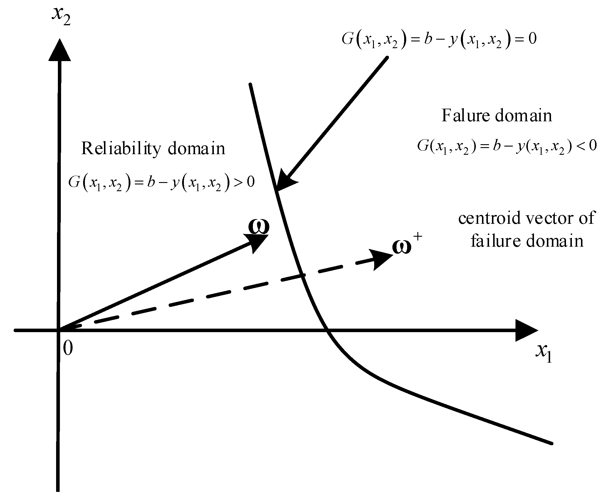
3.1. Polar Transformation For State Function with Randomness and Intervals

The structural state function is defined as:

$$G(x,z)=b-y(x,z)$$

(7)

where $x=\left(x_1,x_2,\cdots ,x_n),z=(z_1,z_2,\cdots ,z_m\right)$ is the basic uncertain vectors of $G(x,z)$. $x_1,x_2,\cdots ,x_n$ are random variables and $z_1,z_2,\cdots ,z_m$ are interval variables. $y(x,z)$ is the structural response and $b$ is the threshold for the $y(x,z)$, whose exceeding defines the failure state. The random variables $x=\left(x_1,x_2,\cdots ,x_n\right)$ are standard Gaussian transformations into $u=(u_1,u_2,\cdots ,u_n)$, where $\forall u_i=T_{random}(x_i)~N(0,1)$, $i=1,2,\cdots ,n$, and $T_{random}(•)$ denotes the standard independent Gaussian transformation that converts $x$ into $u$. The interval variables $z=\left(z_1,z_2,\cdots ,z_m\right)$ are normalized into $\mathsf{\delta }=({\delta }_1,{\delta }_2,\cdots ,{\delta }_m)$, where $\forall {\delta }_j=T_{\mathrm{int}erval}(z_j)\in [-1,1]$, $j=1,2,\cdots ,m$, and $T_{\mathrm{int}erval}(•)$ denotes the standard independent interval transformation that converts $z$ into $\mathsf{\delta }$. Hence, we denote $\mathsf{\omega }=(T_{random}(x),T_{\mathrm{int}erval}(z))=\left(u_1,u_2,\cdots ,u_n,{\delta }_1,{\delta }_2,\cdots ,{\delta }_m\right)$. (7) can be expressed as follows:

$$G(\mathsf{\omega })=b-y(\mathsf{\omega })$$

(8)

In this paper, the polar coordinate is improved. The polar axis is set as the cosine of the angle between the mass center vector of the failure domain and the sample point in a rectangular coordinate system. The pole is the coordinate origin. It is denoted that $v_2=\cos \theta$, $\theta =\angle (\mathsf{\omega },{\mathsf{\omega }}^{+})$, where ${\mathsf{\omega }}^{+}$ is the centroid vector of a failure domain in cartesian coordinate [45], as shown in Figure 1.

Figure 1 suggests that ${\mathsf{\omega }}^{+}$ is paralleled with the gradient direction of state function $G(\mathsf{\omega })$. ${\mathsf{\omega }}^{+}$ denotes the unit vector of $G(\mathsf{\omega })$ at the design point along the gradient direction. The distance $\parallel {\mathsf{\omega }}^{+}\parallel = 1$:

$${\mathsf{\omega }}^{+}=\frac{\nabla G({\mathsf{\omega }}^{*})}{\Vert \nabla G{(\mathsf{\omega })}^{*}\Vert }=-\frac{\nabla y({\mathsf{\omega }}^{*})}{\Vert y{(\mathsf{\omega })}^{*}\Vert }$$

(9)

$${\overline{v}}_1=\sqrt{{\displaystyle \sum _{i=1}^n{u}_i{}^2}+{\displaystyle \sum _{j=1}^m{\delta }_i{}^2}}$$

(10)

$${\overline{v}}_2=\cos \theta =\frac{(\mathsf{\omega },{\mathsf{\omega }}^{+})}{\Vert \mathsf{\omega }\Vert \Vert {\mathsf{\omega }}^{+}\Vert }=\frac{(\mathsf{\omega },{\mathsf{\omega }}^{+})}{\Vert \mathsf{\omega }\Vert \Vert w\Vert }=\frac{(\mathsf{\omega },{\mathsf{\omega }}^{+})}{{\overline{v}}_1}$$

(11)

(8) is rewritten in the polar space as:

$$G({\overline{v}}_1,{\overline{v}}_2)=b-y({\overline{v}}_1,{\overline{v}}_2)$$

(12)

for $\forall n\in N$, it is suggested that:

$$\sqrt{{\displaystyle \sum _{i=1}^n{u}_i{}^2}}\le {\overline{v}}_1=\sqrt{{\displaystyle \sum _{i=1}^n{u}_i{}^2}+{\displaystyle \sum _{j=1}^m{\delta }_i{}^2}}\le \sqrt{{\displaystyle \sum _{i=1}^n{u}_i{}^2}+m}$$

(13)

We denote $\Delta ={\displaystyle \sum _{j=1}^m{\delta }_i{}^2}$, and for $\forall u_i,i=1,2,\cdots ,n$, $u_i$ obeys standard Gaussian distribution. It is reduced so that ${\overline{v}}_1{}^2-\Delta ={\displaystyle \sum _{i=1}^n{u}_i{}^2},\Delta \in [0,m]$, in which ${\displaystyle \sum _{i=1}^n{u}_i{}^2}\sim {\chi }^2(n)$, where $n$ is the number of random variables and $m$ is one of the intervals. Comparing the mean and variance of ${\displaystyle \sum _{i=1}^n{u}_i{}^2}$ and ${\overline{v}}_1{}^2$, it is seen that the shape of the ${\chi }^2$ distribution remains unchanged with the fixed number of random variables (the variance remains unchanged), but the position changes (the mean value changes) with the increase of the number of interval uncertain variables.

Hence, for $\forall \Delta \in [0,m]$, where $m$ represents the number of interval variables, according to (5), the PDF of ${\overline{v}}_1$ is written as:

$$f_{{\overline{v}}_1}(x)=\frac{2^{1-n/2}{(x^2-\Delta )}^{(n-1)/2}}{\Gamma (n/2)}\exp (-\frac{x^2-\Delta }{2})\begin{array}{cc}& \end{array}(x\ge \sqrt{\Delta },\Delta \in [0,m])$$

(14)

The Cumulative Distribution Function (CDF) $F_{v_1}(x,\Delta )$ of ${\overline{v}}_1{}^2$ is nonincreasing for the variable $\Delta$, which is proved by Zhang [22].

With (11), the PDF of $v_2$ is seen as follows:

$$f_{{\overline{v}}_2}(x)=\frac{1}{\sqrt{1-x^2}{\displaystyle {\int }_0^{\pi }{\sin }^{n+m-2}\alpha }d\alpha }({\sin }^{n+m-2}(\arccos x)+{\sin }^{n+m-2}(\pi -\arccos x))$$

(15)

As v₁ and v₂ are independent of each other in the polar coordinate [23], for $G({\overline{v}}_1,{\overline{v}}_2)$, the failure probability $P_{failure}$ in the structure is deduced:

$$P_{failure}(\Delta )=\underset{{\mathsf{\Omega }}_v=\left\{\overline{v}\right|G({\xi }_1,{\xi }_2)\le 0\}}{{\displaystyle {\int }_{-1}^1{\displaystyle {\int }_{\sqrt{\Delta }}^{+\infty }}}}{f}_{{\overline{v}}_1}({\xi }_1,\Delta )f_{{\overline{v}}_2}({\xi }_2)d{\xi }_{1}d{\xi }_2,\Delta \in [0,m]$$

(16)

where $f_{{\overline{v}}_1}$ and $f_{{\overline{v}}_2}$ obey (14) and (15), respectively.

Considering the nonincreasing of ${\overline{v}}_1$ for $\Delta$, when $\Delta =m$, $P_{failure}$ is the minimum value which is written:

$$P_{{}_{failure}}^L=\underset{{\mathsf{\Omega }}_v=\left\{\overline{v}\right|G({\xi }_1,{\xi }_2)\le 0\}}{{\displaystyle {\int }_{-1}^1{\displaystyle {\int }_{\sqrt{m}}^{+\infty }}}}{f}_{{\overline{v}}_1}({\xi }_1,m)f_{{\overline{v}}_2}({\xi }_2)d{\xi }_{1}d{\xi }_2$$

(17)

When $\Delta =0$, $P_{failure}$ is the maximum value which is written:

$$P_{{}_{failure}}^U=\underset{{\mathsf{\Omega }}_v=\left\{\overline{v}\right|G({\xi }_1,{\xi }_2)\le 0\}}{{\displaystyle {\int }_{-1}^1{\displaystyle {\int }_0^{+\infty }}}}{f}_{{\overline{v}}_1}({\xi }_1)f_{{\overline{v}}_2}({\xi }_2)d{\xi }_{1}d{\xi }_2$$

(18)

where $f_{{\overline{v}}_1}$ and $f_{{\overline{v}}_2}$ obey (14) and (15), respectively.

Finally, the interval of $P_{failure}$ can be calculated as $P_{failure}^L, P_{failure}^U$.

3.2. UPSORM: SORM in Polar for Random and Interval Uncertainty

Assuming that the design point at the failure domain of the structure is ${\mathsf{\omega }}^{*}=(u^{*}{}_1,u^{*}{}_2,\cdots ,u^{*}{}_n,{\delta }_1{}^{*},{\delta }_2{}^{*},\cdots ,{\delta }_m{}^{*})$, the second-order Taylor expansion of $G(\mathsf{\omega })$ at the design point ${\mathsf{\omega }}^{*}$ is described as:

$$G(\mathsf{\omega })\approx G({\mathsf{\omega }}^{*})+\nabla G({\mathsf{\omega }}^{*})(\mathsf{\omega }-{\mathsf{\omega }}^{*})+\frac{1}{2}{(\mathsf{\omega }-{\mathsf{\omega }}^{*})}^{T}H(\mathsf{\omega }-{\mathsf{\omega }}^{*})$$

(19)

where $\nabla G({\mathsf{\omega }}^{*})$ is the gradient of $G(\mathsf{\omega })$ with $\nabla G({\mathsf{\omega }}^{*})={\frac{\partial G}{\partial \mathsf{\omega }}|}_{{\mathsf{\omega }}^{*}}$, $H$ is the Hessian matrix, written as $H_{ij}={\frac{\partial G}{\partial {\omega }_i\partial {\omega }_j}|}_{{\mathsf{\omega }}^{*}}$. Then, (19) is simplified as:

$$\begin{array}{cc}\hfill G(\mathsf{\omega })& \approx b-y({\mathsf{\omega }}^{*})-\nabla y({\mathsf{\omega }}^{*})(\mathsf{\omega }-{\mathsf{\omega }}^{*})-\lambda {(\mathsf{\omega }-{\mathsf{\omega }}^{*})}^T(\mathsf{\omega }-{\mathsf{\omega }}^{*})\hfill \\ & =b-y({\mathsf{\omega }}^{*})+{\displaystyle \sum _{k=1}^{n+m}\left({\frac{\partial y}{\partial {\omega }_k}|}_{{\mathsf{\omega }}^{*}}{\omega }_k{}^{*}\right)}-{\displaystyle \sum _{k=1}^{n+m}\left({\frac{\partial y}{\partial {\omega }_k}|}_{{\mathsf{\omega }}^{*}}{\omega }_k\right)}\hfill \\ & +2\lambda {\displaystyle \sum _{k=1}^{n+m}{\omega }_k{\omega }_k{}^{*}}-\lambda {\displaystyle \sum _{k=1}^{n+m}{\left({\omega }_k{}^{*}\right)}^2}-\lambda {\displaystyle \sum _{k=1}^{n+m}{\omega }_k{}^2}\hfill \end{array}$$

(20)

where $\lambda$ is a constant parameter. Obviously, ${\mathsf{\omega }}^{*}=\Vert {\mathsf{\omega }}^{*}\Vert {\mathsf{\omega }}^{+}$, hence, ${\displaystyle \sum _{k=1}^{n+m}{\omega }_k{\omega }_k{}^{*}}=\frac{{\displaystyle \sum _{k=1}^{n+m}{\omega }_k{\omega }_k{}^{+}}}{\Vert {\omega }_k{}^{*}\Vert }$.

Then, (20) is written as:

$$\begin{array}{cc}\hfill G(\mathsf{\omega })& =b-y({\mathsf{\omega }}^{*})+{\displaystyle \sum _{k=1}^{n+m}\left({\frac{\partial y}{\partial {\omega }_k}|}_{{\mathsf{\omega }}^{*}}{\omega }_k{}^{*}\right)}-{\displaystyle \sum _{k=1}^{n+m}\left({\frac{\partial y}{\partial {\omega }_k}|}_{{\mathsf{\omega }}^{*}}{\omega }_k\right)}\hfill \\ & +\frac{2\lambda }{\Vert {\omega }_k{}^{*}\Vert {\left[{\displaystyle \sum _{k=1}^{n+m}{\left({\frac{\partial y}{\partial {\omega }_i}|}_{{\mathsf{\omega }}^{*}}\right)}^2}\right]}^{1/2}}{\displaystyle \sum _{k=1}^{n+m}{\frac{\partial y}{\partial {\omega }_k}|}_{{\mathsf{\omega }}^{*}}{\omega }_k}-\lambda {\displaystyle \sum _{k=1}^{n+m}{\left({\omega }_k{}^{*}\right)}^2}-\lambda {\displaystyle \sum _{k=1}^{n+m}{\omega }_k{}^2}\hfill \end{array}$$

(21)

Denote $v_1$ and $v_2$:

$$v_1=\sqrt{{\displaystyle \sum _{k=1}^{n+m}{\omega }_i^2}}=\sqrt{{\displaystyle \sum _{i=1}^n{u}_i^2}+{\displaystyle \sum _{j=1}^m{\delta }_i^2}}$$

(22)

$$v_2=\cos \angle ({\mathsf{\omega }}^{+},\mathsf{\omega })=\frac{{\displaystyle \sum _{k=1}^{n+m}\left({\frac{\partial y}{\partial {\omega }_i}|}_{{\mathsf{\omega }}^{*}}{\omega }_i\right)}}{v_1{\left[{\displaystyle \sum _{k=1}^{n+m}{\left({\frac{\partial y}{\partial {\omega }_i}|}_{{\mathsf{\omega }}^{*}}\right)}^2}\right]}^{1/2}}=\frac{{\displaystyle \sum _{i=1}^n\left({\frac{\partial y}{\partial u_i}|}_{{\mathsf{\omega }}^{*}}{u}_i\right)}+{\displaystyle \sum _{j=1}^m\left({\frac{\partial y}{\partial {\delta }_j}|}_{{\mathsf{\omega }}^{*}}{\delta }_j\right)}}{v_1{\left[{\displaystyle \sum _{i=1}^n{\left({\frac{\partial y}{\partial u_i}|}_{{\mathsf{\omega }}^{*}}\right)}^2+{\displaystyle \sum _{j=1}^m{\left({\frac{\partial y}{\partial {\delta }_j}|}_{{\mathsf{\omega }}^{*}}\right)}^2}}\right]}^{1/2}}$$

(23)

In polar space, involving functions (21) and (22), the state function (24) is expressed as follows:

$$G(v_1,v_2)=b-y({\mathsf{\omega }}^{*})+{\displaystyle \sum _{k=1}^{n+m}\left({\frac{\partial y}{\partial {\omega }_k}|}_{{\mathsf{\omega }}^{*}}{\omega }_k{}^{*}\right)}-\lambda v_1^{*}{}^2+\left(\frac{2\lambda }{v_1^{*}}-D\right)v_1{v}_2-\lambda v_1{}^2$$

(24)

Given that $G(v_1{}^{*},v_2{}^{*})=0$, it is observed that:

$$b-y({\mathsf{\omega }}^{*})+{\displaystyle \sum _{k=1}^{n+m}\left({\frac{\partial y}{\partial {\omega }_k}|}_{{\mathsf{\omega }}^{*}}{\omega }_k{}^{*}\right)}+2\lambda v_2^{*}-D{v}_1{}^{*}{v}_2{}^{*}-2\lambda v_1{{}^{*}}^2=0$$

(25)

$$\lambda =\frac{b-y({\mathsf{\omega }}^{*})+{\displaystyle \sum _{k=1}^{n+m}\left({\frac{\partial y}{\partial {\omega }_k}|}_{{\mathsf{\omega }}^{*}}{\omega }_k{}^{*}\right)}-D{v}_1{}^{*}{v}_2{}^{*}}{2v_1{{}^{*}}^2-2v_2^{*}}$$

(26)

where $D={\left[{\displaystyle \sum _{k=1}^{n+m}{\left({\frac{\partial y}{\partial {\omega }_i}|}_{{\mathsf{\omega }}^{*}}\right)}^2}\right]}^{1/2}={\left[{\displaystyle \sum _{i=1}^n{\left({\frac{\partial y}{\partial u_i}|}_{{\mathsf{\omega }}^{*}}\right)}^2+{\displaystyle \sum _{j=1}^m{\left({\frac{\partial y}{\partial {\delta }_j}|}_{{\mathsf{\omega }}^{*}}\right)}^2}}\right]}^{1/2}$.

Then, (24) can be written as

$$G(v_1,v_2)=d+\left(\frac{2\lambda }{v_1^{*}}-D\right)v_1{v}_2-\lambda v_1{}^2$$

(27)

where $\lambda =\frac{b-y({\mathsf{\omega }}^{*})+{\displaystyle \sum _{k=1}^{n+m}\left({\frac{\partial y}{\partial {\omega }_k}|}_{{\mathsf{\omega }}^{*}}{\omega }_k{}^{*}\right)}-D{v}_1{}^{*}{v}_2{}^{*}}{2v_1{{}^{*}}^2-2v_2^{*}}$, $d=b-y({\mathsf{\omega }}^{*})+{\displaystyle \sum _{k=1}^{n+m}\left({\frac{\partial y}{\partial {\omega }_k}|}_{{\mathsf{\omega }}^{*}}{\omega }_k{}^{*}\right)}-\lambda v_1^{*}{}^2$, and $D={\left[{\displaystyle \sum _{k=1}^{n+m}{\left({\frac{\partial y}{\partial {\omega }_i}|}_{{\mathsf{\omega }}^{*}}\right)}^2}\right]}^{1/2}={\left[{\displaystyle \sum _{i=1}^n{\left({\frac{\partial y}{\partial u_i}|}_{{\mathsf{\omega }}^{*}}\right)}^2+{\displaystyle \sum _{j=1}^m{\left({\frac{\partial y}{\partial {\delta }_j}|}_{{\mathsf{\omega }}^{*}}\right)}^2}}\right]}^{1/2}$.

In polar space, the new reliability domain is $d+\left(\frac{2\lambda }{v_1^{*}}-D\right)v_1{v}_2-\lambda v_1{}^2>0$, and the failure domain is $d+\left(\frac{2\lambda }{v_1^{*}}-D\right)v_1{v}_2-\lambda v_1{}^2\le 0$. The limit stat surface is:

$$d+\left(\frac{2\lambda }{v_1^{*}}-D\right)v_1{v}_2-\lambda v_1{}^2=0$$

(28)

By functions (18) and (19), it is obtained that:

$$P_R^U=1-\underset{{\mathsf{\Omega }}_v=\left\{v\right|d-\lambda v_1^{*}{}^2+\left(\frac{2\lambda }{v_1^{*}}-D\right){\xi }_1{\xi }_2-\lambda {\xi }_1{}^2\le 0\}}{{\displaystyle {\int }_{\sqrt{m}}^{+\infty }{\displaystyle {\int }_{-1}^1}}}{f}_{v_1}({\xi }_1)f_{v_2}({\xi }_2)d{\xi }_{1}d{\xi }_2$$

(29)

where $f_{v_1}(x)=\frac{2^{1-n/2}{(x_{}^2-m)}^{(n-1)/2}}{\Gamma (n/2)}\exp (-\frac{x^2-m}{2})$, and

$f_{v_2}(x)=\frac{1}{\sqrt{1-x^2}{\displaystyle {\int }_0^{\pi }{\sin }^{n+m-2}\alpha }d\alpha }({\sin }^{n+m-2}(\arccos x)+{\sin }^{n+m-2}(\pi -\arccos x))$,

$$P_R^L=1-\underset{{\mathsf{\Omega }}_v=\left\{v\right|d-\lambda v_1^{*}{}^2+\left(\frac{2\lambda }{v_1^{*}}-D\right){\xi }_1{\xi }_2-\lambda {\xi }_1{}^2\le 0\}}{{\displaystyle {\int }_0^{+\infty }{\displaystyle {\int }_{-1}^1}}}{f}_{v_1}({\xi }_1)f_{v_2}({\xi }_1)d{\xi }_{1}d{\xi }_2$$

(30)

where $f_{v_1}(x)=\frac{2^{1-n/2}{x}^{(n-1)}}{\Gamma (n/2)}\exp (-\frac{x^2}{2})$, and

$f_{v_2}(x)=\frac{1}{\sqrt{1-x^2}{\displaystyle {\int }_0^{\pi }{\sin }^{n+m-2}\alpha }d\alpha }({\sin }^{n+m-2}(\arccos x)+{\sin }^{n+m-2}(\pi -\arccos x))$.

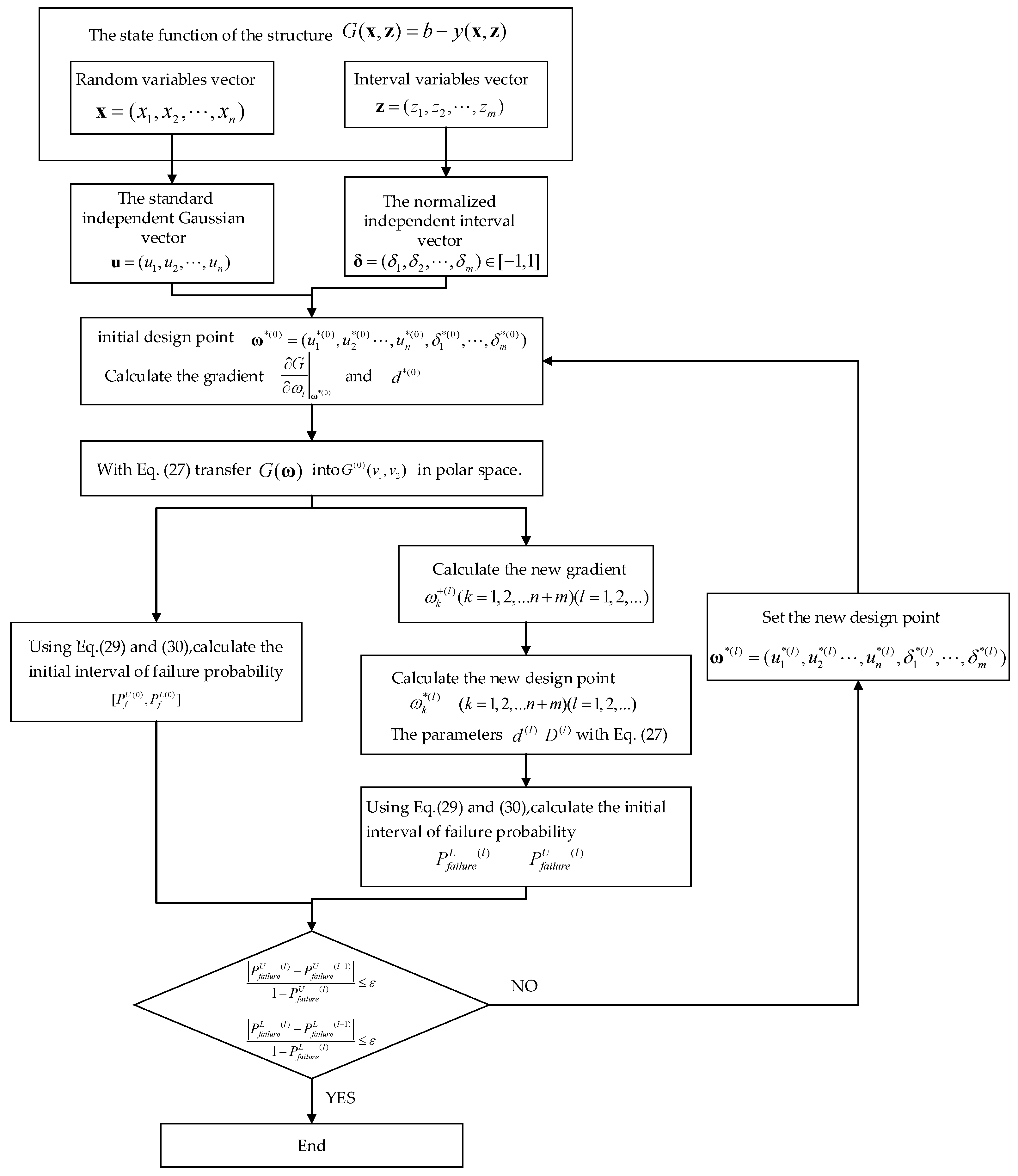
3.3. Implementation Details

(1) For the random variables vector $x=(x_1,x_2,\cdots ,x_n)$ and interval variables vector $z=(z_1,z_2,\cdots ,z_m)$, $z_j\in [z_{{}_j}^L,z_{{}_j}^U]$ in the state function of the structure $G(x,z)=b-y(x,z)$, transfer $x$ to the independent Gaussian vector $u=(u_1,u_2,\cdots ,u_n)$ and convert $z$ to the independent normalized interval vector $\mathsf{\delta }=({\delta }_1,{\delta }_2,\cdots ,{\delta }_m)\in [-1,1]$. Then, $G(x,z)$ is converted into $G(\mathsf{\omega })$ with $\mathsf{\omega }=(u,\mathsf{\delta })$.

(2) Given an initial design point ${\mathsf{\omega }}_{}^{*(0)}=(u_1^{*(0)},u_2^{*(0)}\cdots ,u_n^{*(0)},{\delta }_1^{*(0)},\cdots ,{\delta }_m^{*(0)})$, compute the gradient ${\frac{\partial G}{\partial {\omega }_i}|}_{{\mathsf{\omega }}^{*(0)}}$ of $G(\mathsf{\omega })$, $d^{*(0)}$ and $D^{*(0)}$ at ${\mathsf{\omega }}_{}^{*(0)}$, and with Equation (27) transfer $G(\mathsf{\omega })$ into $G^{(0)}(v_1,v_2)$ in polar space.

(3) Using Equations (29) and (30), compute the initial failure probability interval $[P_f^U{}^{(0)},P_f^L{}^{(0)}]$.

(4) Compute ${\omega }_k^{+}{}^{(l)}(k=1,2,\dots n+m)(l=1,2,\dots )$ by Equation (31)

$${\omega }_k^{+}{}^{(l)}=\frac{{-\frac{\partial y}{\partial {\omega }_k}|}_{{\mathsf{\omega }}_k{}^{*(l-1)}}}{{\left[{\displaystyle \sum _{k=1}^{n+m}{\left({\frac{\partial y}{\partial {\omega }_k}|}_{{\mathsf{\omega }}_k{}^{*(l-1)}}\right)}^2}\right]}^{1/2}}(l=1,2,\dots )$$

(31)

(5) Calculate the new design point ${\omega }_k^{*(l)}$$(k=1,2,\dots n+m)(l=1,2,\dots )$ with ${\omega }_k^{+}{}^{(l)}$ by function (32)

$${\omega }_k^{*(l)}={\omega }_k^{*(l-1)}+\Vert {\omega }_k^{*(l-1)}\Vert {\omega }_k^{+}{}^{(l)}={\omega }_k^{*(l-1)}+\Vert {\omega }_k^{*(l-1)}\Vert \frac{{-\frac{\partial y}{\partial {\omega }_k}|}_{{\mathsf{\omega }}_k{}^{*(l-1)}}}{{\left[{\displaystyle \sum _{k=1}^{n+m}{\left({\frac{\partial y}{\partial {\omega }_k}|}_{{\mathsf{\omega }}_k{}^{*(l-1)}}\right)}^2}\right]}^{1/2}}(l=1,2,\dots )$$

(32)

and parameters $d^{(l)}$ and $D^{(l)}$ with Equation (27).

(6) Compute the failure probability interval $P_{failure}^L{}^{(l)}$ and $P_{failure}^U{}^{(l)}$ with Equations (29) and (30). Taking the robust convergence into account, assume that the iterative errors are denoted as $\frac{\left|P_{failure}^U{}^{(l)}-P_{failure}^U{}^{(l-1)}\right|}{1-P_{failure}^U{}^{(l)}}$ and $\frac{\left|P_{failure}^L{}^{(l)}-P_{failure}^L{}^{(l-1)}\right|}{1-P_{failure}^{lower}{}^{(l)}}$. The thresholds of them is $\epsilon$. If $\frac{\left|P_{failure}^U{}^{(l)}-P_{failure}^U{}^{(l-1)}\right|}{1-P_{failure}^U{}^{(l)}}\le \epsilon$ and $\frac{\left|P_{failure}^L{}^{(l)}-P_{failure}^L{}^{(l-1)}\right|}{1-P_{failure}^{lower}{}^{(l)}}\le \epsilon$, stop the calculating procedure. Otherwise, repeat steps 2–6. Assign the design point ${\mathsf{\omega }}_{}^{*(l)}=(u_1^{*(l)},u_2^{*(l)}\cdots ,u_n^{*(l)},{\delta }_1^{*(l)},\cdots ,{\delta }_m^{*(l)})$ by the initial design point until the accuracy requirement is satisfied. The main steps for implementation are shown in Figure 2. The pseudo-code that illustrates the process of using the method in more detail is shown in Appendix A.

4. Numerical Examples

4.1. A Toy Example

Assume that there is a tension $P$ that forces on a round bar. The diameter of the bar $D$ is a random variable, obeying the normal distribution with the mean ${\mu }_D=29.4$ m and variance ${\sigma }_D=3$. The tension $P$ is an interval variable with $P\in [30KN,90KN]$, $P$ and $D$ are independent and the material strength R = 170 MPa, is a constant. In the original space, the state function $G\left(P,D\right)=170-\frac{4P}{\pi D^2}$, and in standard normal space, the function is written as:

$$F\left(\delta ,u\right)=170-\frac{120000\times (\delta +2)}{\pi {\left(3u+29.4\right)}^2}$$

(33)

where $P$ is standard interval transformed into $\delta$ in which $\delta \in [-1,1]$, and $D$ is standard Gaussian transformed into $u$, which obeys standard Gaussian distribution $N(0,1)$.

In this paper, the accuracy of the UPSORM is compared with the new FORM by Qiu [22] and MC (10⁷ samples). The comparison results are summarized in

Table 1. Comparison result.

Method	Failure Probability Interval		Relative Error
	Lower Boundary	Upper Boundary	Lower Boundary	Upper Boundary
MC(107)	0.0591	0.4421
Uncertainty FORM in [22]	0.0537	0.4672	9.13%	5.68%
UPSORM	0.0634	0.4192	7.28%	5.18%

.

It is found that the proposed method produces better estimation results. In general, it outperforms Qiu’s method [22] both in accuracy and efficiency, though the improvement is not significant since the limit-state function is relatively simple.

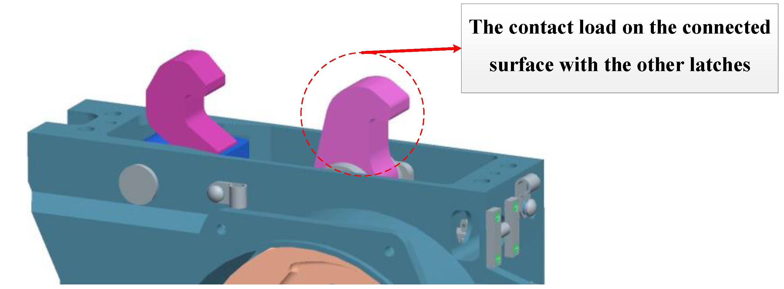
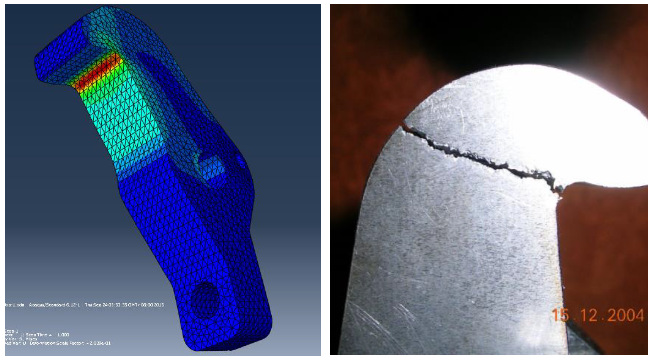
4.2. A Pracitical Application Example—Space Docking Mechanism

In the space docking mechanism, the docking lock is a key component which realizes the rigid connection and separation of the spacecraft, as shown in Figure 3. With the interaction of the docking lock system on the two spacecrafts the connection force is generated/released between the two spacecrafts and the rigid connection or separation is realized. Each set of locks is composed of an active lock hook and a passive lock hook. The active lock hook is driven by a motor and matches with the passive lock hook corresponding to the target spacecraft. The passive lock hook is installed on the disc spring to match with the active lock hook corresponding to the target spacecraft [22].

The load $F$ is defined as an interval variable that ranges $\left[30KN,40KN\right]$ the structural locking latch. The elastic modulus of the material E, Poisson’s ratio $\mu$, and the density $\rho$ are random variables shown in

Table 2. The list of random variables.

Random Variables	Distribution Type	Mean	Standard Deviation
elastic modulus E (Pa)	normal	117 × 109	117 × 107
Poisson’s ratio $\mu$	normal	0.3	0.003
density $\rho$ (kg/m3)	normal	4.81 × 103	0.481 × 103

.

The reliability problem is formulated using the state function as:

$$g=b-y(F,E,\mu ,\rho )$$

where $b$ indicates the yield strength (1300 Mpa), and the contact stress $y(F,E,\mu ,\rho )$ on the connective surface of the two latches. Note that the four independent random variables are assumed and the max value of the contact stress $y(F,E,\mu ,\rho )$ is a function of the four variables $F,E,\mu ,\rho$, which cannot be an explicit expression. A simplified model for a finite element analysis is established to estimate the max contact stress $y(F,E,\mu ,\rho )$, as shown in Figure 4, which is the data of the red area in the left figure. In order to ensure the accuracy of the collected data, the test is used, and it is suggested that the damage position of the structure (the right picture) is the distribution area of the maximum contact stress (the left picture), which verifies the correctness of the collected data in this case

In this case, the new method is employed to compute the failure probability of the latch, comparing the result to the computation made by the MC method with 10⁷ samples to evaluate the accuracy of the calculation results. The results are shown in

Table 3. The comparison of lower and upper bounds.

Method	Failure Probability Interval		Relative Error
	Lower Boundary	Upper Boundary	Lower Boundary	Upper Boundary
MC (${10}^7$)	$3.9120\times {10}^{-6}$	$4.7801\times {10}^{-5}$	/	/
Uncertainty FORM in [22]	$4.3580\times {10}^{-6}$	$4.3930\times {10}^{-5}$	11.4%	8.12%
UPSORM	$4.2203\times {10}^{-6}$	$4.4190\times {10}^{-5}$	7.88%	7.55%

.

Table 3 summarizes the estimation results for the structural latch computed by Monte Carlo (MC) simulation, the uncertainty FORM, and the proposed UPSORM. As shown in Table 3, the lower and upper bounds are computed for the failure probability: [$4.2203\times {10}^{-6}$, $4.4190\times {10}^{-5}$], which is measured by the proposed UPSORM after 154 iterations. It is matched to the results obtained by the MC simulation, showing that all the failure samples were correctly identified. Yet, the relative errors of 7.88% and 7.55% mean that the adoption of the second-order Taylor expansion improves the efficiency with a tradeoff in estimation accuracy.

The lower and upper boundaries between the MC and UPSORM are different, as shown in Table 3, induced by the nonlinear limit-state function. The relative errors of 7.55% and 7.88%, respectively, are within acceptable ranges for the upper and lower bounds. Comparing the relative errors of the FORM in Qiu [22] shows the direct influences of the nonlinearity to the estimation accuracy. The second-order Taylor series is better than the linear one in resolving the structural reliability problem with nonlinear limit-state function.

5. Conclusions

This paper proposes a unified reliability framework to address the reliability of a complex system in the presence of both stochastic and interval variables. On the aggregation of different uncertain variables, a novel SORM method, UPSORM, is proposed. By introducing a novel polar transformation technique, a multivariate limit-state function is reformulated as a generalized bivariate limit-state function in the polar coordinate. For this purpose, we set the gradient direction of the limit-state function as the polar coordinate. In this manner, the computational cost is significantly reduced as the original n-dimensional reliability problem is simplified to a two-dimensional problem.

The proposed method was evaluated through a numerical case study. The upper and lower bounds of reliability were estimated. To further validate its practical feasibility, a real engineering case was employed as an application example. The proposed method was compared with the classical MC algorithm and the state-of-the-art method, showing that the proposed method provides comparable results with lower computational costs. In particular, the proposed method outperformed the compared methods for cases with strong nonlinearity.

References

1. Wang, P.; Zhang, J.; Zhai, H.; Qiu, J. A new structural reliability index based on uncertainty theory. Chin. J. Aeronaut. 2017, 30, 1451–1458. [Google Scholar] [CrossRef]
2. Ekin, O.; Maria, Q.F. Structural Reliability Estimation with Participatory Sensing and Mobile Cyber-Physical Structural Health Monitoring Systems. Appl. Sci. 2019, 9, 2840. [Google Scholar]
3. Dai, W.; Chi, Y.; Lu, Z.; Wang, M.; Zhao, Y. Research on reliability assessment of mechanical equipment based on the performance-feature model. Appl. Sci. 2018, 8, 1619. [Google Scholar] [CrossRef] [Green Version]
4. Huang, P.; Huang, H.Z.; Huang, T. A Novel Algorithm for Structural Reliability Analysis Based on Finite Step Length and Armijo Line Search. Appl. Sci. 2019, 9, 2546. [Google Scholar] [CrossRef] [Green Version]
5. Cheng, J.; Zhang, Y.; Feng, Y.; Liu, Z.; Tan, J. Structural optimization of a high-speed Press considering multi-source uncertainties based on a new heterogeneous TOPSIS. Appl. Sci. 2018, 8, 126. [Google Scholar] [CrossRef] [Green Version]
6. Melchers, R.E. Structural Reliability Analysis and Prediction, 2nd ed.; John Wiley: New York, NY, USA, 1999; pp. 9–62. [Google Scholar]
7. Yang, L.; Guo, Y.; Wang, Q. Reliability assessment of a hierarchical system subjected to inconsistent priors and multi-level data. IEEE Trans. Reliab. 2020, 69, 277–292. [Google Scholar] [CrossRef]
8. Rackwitz, R. Reliability analysis–A review and some perspectives. Struct. Saf. 2001, 23, 365–395. [Google Scholar] [CrossRef]
9. Zhao, Y.G.; Ono, T. A general procedure for first/second-order reliability method (FORM/SORM). Struct. Saf. 1999, 21, 95–112. [Google Scholar] [CrossRef]
10. Abdelouafi, E.G.; Benaissa, K.; Abdellatif, K. Reliability analysis of reinforced concrete buildings: Comparison between FORM and ISM. Procedia Eng. 2015, 114, 650–657. [Google Scholar] [CrossRef] [Green Version]
11. Huang, X.; Li, Y.; Zhang, Y.; Zhang, X. A new direct second-order reliability analysis method. Appl. Math. Model. 2018, 55, 68–80. [Google Scholar] [CrossRef]
12. Yang, L.; Guo, Y. Combining pre- and post-model information in the uncertainty quantification of non-deterministic models using an extended Bayesian melding approach. Inf. Sci. 2019, 502, 146–163. [Google Scholar] [CrossRef]
13. Yang, L.; Guo, Y.; Kong, Z. On the performance evaluation of a hierarchical-structure prototype product using inconsistent prior information and limited test data. Inf. Sci. 2019, 485, 362–375. [Google Scholar] [CrossRef]
14. Breitung, K. 40 years FORM: Some new aspects? Probablist. Eng. Mech. 2015, 42, 71–77. [Google Scholar] [CrossRef]
15. Wang, W.; Xue, H.; Kong, T. An efficient hybrid reliability analysis method for structures involving random and interval variables. Struct. Multidiscip. Optim. 2020, 62, 1–2. [Google Scholar] [CrossRef] [Green Version]
16. Low, B.K. FORM, SORM, and spatial modeling in geotechnical engineering. Struct. Saf. 2014, 49, 56–64. [Google Scholar] [CrossRef]
17. Lu, Z.H.; Hu, D.Z.; Zhao, Y.G. Second-order fourth-moment method for structural reliability. J. Eng. Mech. 2017, 143. [Google Scholar] [CrossRef]
18. Zeng, P.; Li, T.; Jimenez, R.; Feng, X.D.; Chen, Y. Extension of quasi-Newton approximation-based SORM for series system reliability analysis of geotechnical problems. Eng. Comput. 2018, 34, 215–224. [Google Scholar] [CrossRef]
19. Mansour, R.; Olsson, M. A closed-form second-order reliability method using noncentral chi-squared distributions. J. Mech. Des. 2014, 136, 1–10. [Google Scholar] [CrossRef]
20. Yoo, D.; Lee, I.; Cho, H. Probabilistic sensitivity analysis for novel second-order reliability method (SORM) using generalized chi-squared distribution. Struct. Multidiscip. Optim. 2014, 50, 787–797. [Google Scholar] [CrossRef]
21. Kiureghian, A.D.; Ditlevsen, O. Aleatory or epistemic? Does it matter? Struct. Saf. 2009, 31, 105–112. [Google Scholar] [CrossRef]
22. Zhang, J.; Qiu, J.; Wang, P. Hybrid Reliability Analysis for Spacecraft Docking Lock with Random and Interval Uncertainty. Int. J. Aerosp. Eng. 2017, 2017, 3920267. [Google Scholar] [CrossRef] [Green Version]
23. Hurtado, J.E.; Alvarez, D.A. The encounter of interval and probabilistic approaches to structural reliability at the design point. Comput. Methods Appl. Mech. Eng. 2012, 225, 74–94. [Google Scholar] [CrossRef]
24. Zaman, K.; Rangavajhala, S.; Mcdonald, M.P.; Mahadevan, S. A probabilistic approach for representation of interval uncertainty. Reliab. Eng. Syst. Saf. 2011, 96, 117–130. [Google Scholar] [CrossRef]
25. Wang, L.; Wang, X.; Xia, Y. Hybrid reliability analysis of structures with multi-source uncertainties. Acta Mech. 2014, 225, 413–430. [Google Scholar] [CrossRef] [Green Version]
26. Xiao, M.; Zhang, J.; Gao, L.; Lee, S.; Eshghi, A.T. An efficient Kriging-based subset simulation method for hybrid reliability analysis under random and interval variables with small failure probability. Struct. Multidiscip. Optim. 2019, 59, 2077–2092. [Google Scholar] [CrossRef]
27. Penmetsa, R.C.; Grandhi, R.V. Efficient estimation of structural reliability for problems with uncertain intervals. Comput. Struct. 2002, 80, 1103–1112. [Google Scholar] [CrossRef]
28. Sankararaman, S.; Mahadevan, S. Separating the contributions of variability and parameter uncertainty in probability distributions. Reliab. Eng. Syst. Saf. 2013, 112, 187–199. [Google Scholar] [CrossRef]
29. Alvarez, D.A.; Hurtado, J.E. An efficient method for the estimation of structural reliability intervals with random sets, dependence modeling and uncertain inputs. Comput. Struct. 2014, 142, 54–63. [Google Scholar] [CrossRef]
30. Hurtado, J.E. Assessment of reliability intervals under input distributions with uncertain parameters. Probabilist. Eng. Mech. 2013, 32, 80–92. [Google Scholar] [CrossRef]
31. Hall, J.W.; Lawry, J. Generation, combination and extension of random set approximations to coherent lower and upper probabilities. Reliab. Eng. Syst. Saf. 2004, 85, 89–101. [Google Scholar] [CrossRef]
32. Karanki, D.R.; Kushwaha, H.S.; Verma, A.K.; Ajit, S. Uncertainty analysis based on probability bounds (p-box) approach in probabilistic safety assessment. Risk Anal. 2009, 29, 662–675. [Google Scholar] [CrossRef] [PubMed]
33. Gao, W.; Wu, D.; Song, C.M.; Tin Loi, F.; Li, X. Hybrid probabilistic interval analysis of bar structures with uncertainty using a mixed perturbation Monte-Carlo method. Finite Elem. Anal. Des. 2011, 47, 643–652. [Google Scholar] [CrossRef]
34. Xie, S.J.; Pan, B.S.; Du, X.P. A single-loop optimization method for reliability analysis with second order uncertainty. Eng. Optimiz. 2014, 47, 1125–1139. [Google Scholar] [CrossRef]
35. Yoo, D.; Lee, I. Sampling-based approach for design optimization in the presence of interval variables. Struct. Multidiscip. Optim. 2014, 49, 253–266. [Google Scholar] [CrossRef]
36. Guo, J.; Du, X.P. Reliability sensitivity analysis with random and interval variables. Int. J. Numer. Meth. Eng. 2010, 78, 1585–1617. [Google Scholar] [CrossRef]
37. Luo, Y.J.; Kang, Z.; Li, A. Structural reliability assessment based on probability and convex set mixed model. Comput. Struct. 2009, 87, 1408–1415. [Google Scholar] [CrossRef]
38. Du, X.; Sudjianto, A.; Huang, B. Reliability-Based Design with the Mixture of Random and Interval Variables. J. Mech. Des. 2005, 127, 1068–1076. [Google Scholar] [CrossRef] [Green Version]
39. Qiu, Z.P.; Wang, J. The interval estimation of reliability for probabilistic and non-probabilistic hybrid structural system. Eng. Fail. Anal. 2010, 17, 1142–1154. [Google Scholar] [CrossRef]
40. Chowdhury, R.; Rao, B.N. Hybrid high dimensional model representation for reliability analysis. Comput. Methods Appl. Mech. Eng. 2009, 198, 753–765. [Google Scholar] [CrossRef]
41. Jiang, C.; Han, X.; Liu, W.; Liu, J.; Zhang, Z. A Hybrid Reliability Approach Based on Probability and Interval for Uncertain Structures. J. Mech. Des. 2012, 134, 031001. [Google Scholar] [CrossRef]
42. Kang, Z.; Luo, Y. Reliability-based structural optimization with probability and convex set hybrid models. Struct. Multidiscip. Optim. 2010, 42, 89–102. [Google Scholar] [CrossRef]
43. Xie, S.; Pan, B.; Du, X. An efficient hybrid reliability analysis method with random and interval variables. Eng. Optimiz. 2015, 48, 1–15. [Google Scholar] [CrossRef]
44. Alibrandi, U.; Koh, C.G. First-Order Reliability Method for Structural Reliability Analysis in the Presence of Random and Interval Variables. J. Risk Uncertain. Eng. Syst. Part B Mech. Eng. 2015, 4, 1–10. [Google Scholar] [CrossRef]
45. Hurtado, J.E. Dimensionality reduction and visualization of structural reliability problems using polar features. Probabilist. Eng. Mech. 2012, 29, 16–31. [Google Scholar] [CrossRef]
Figure 1. The diagram of the centroid vector of a failure domain in 2-dimensional space.
Applsci 11 00346 g001
Figure 2. The flowchart of the implementation.
Applsci 11 00346 g002
Figure 3. Space docking mechanism.
Applsci 11 00346 g003
Figure 4. The stress nephogram and test result for the structural latch.
Applsci 11 00346 g004