Image Quality Improvement and Memory-Saving in a Permanent-Magnet-Array-Based MRI System

Abstract

Point-of-care magnetic resonance imaging (MRI) requires clear images within a short scanning time, a small footprint of the scanner, and relatively low memory required for image reconstruction. A permanent magnet array (PMA)-based MRI system is a good candidate to supply a magnetic field due to its compactness and low power consumption. However, it has relatively inhomogeneous magnetic field and thus non-linear gradients, which results in location-dependent k-spaces (so called local k-spaces) and uneven signal point populations in the local k-spaces, compromising the image quality. Moreover, owing to the non-linearity, imaging reconstruction using Fourier transform does not work, which leads to an increase in the required computation memory. In this study, in order to improve the image quality, the approaches of compensating the uneven signal point population by increasing the numbers of sampling points or rotation angles are investigated in terms of their impacts on image quality improvement, acquisition time, image reconstruction time, and memory consumption. Both methods give a significant improvement on image image quality although they result in a large and dense encoding matrix and thus a large memory consumption. To lower the memory consumption, it is further proposed to transform such a matrix to frequency domain where the matrix could be sparse. Moreover, a row-wise truncation to the transformed encoding matrix is applied to further reduce the memory consumption. Through the results of numerical experiments, it is shown that the required memory for calculation can effectively be reduced by 71.6% while the image becomes clearer by increasing the number of sampling point and/or the number of rotation angles. With the successful demonstration where improved image quality and a lowered memory required can be obtained simultaneously, the proposed study is one step forward for a PMA-based MRI system towards its targeted point-of-care application scenario.

1. Introduction

Magnetic resonance imaging (MRI) is a popular imaging modality for diagnosis and therapies. It shows the best soft tissue contrast and has no ionizing radiation. However, a conventional MRI system has been extremely expensive (approaching 1 million USD per Tesla (T) of the main magnetic field (${\mathit{B}}_{\mathbf{0}}$-field)), which significantly limits its accessibility. Moreover, it requires a large space to site. The bulkiness of an MRI scanner prevents this imaging modality from being available to “point-of-care” and timely diagnosis, e.g., those in an ambulance, a field medical tent, or an intensive care unit (ICU). To this end, instead of using a superconducting magnet for a full body which requires a sophisticated and costly cooling system to maintain a superconducting state, body-part-dedicated permanent magnet array (PMA) is drawing more and more attention to be used as a source to supply ${\mathit{B}}_{\mathbf{0}}$-field [1,2,3,4,5,6] because of its low cost, no energy consumption, small footprint, and light weight.

In the linear MRI system such as those for Cartesian or radial imaging, it requires both a highly homogeneous ${\mathit{B}}_{\mathbf{0}}$ and a linear gradient field to ensure image quality and to avoid aliasing. When a PMA is used to supply such a ${\mathit{B}}_{\mathbf{0}}$-field, either the field of view (FoV) becomes small to guarantee a relatively high field strength and the homogeneity, or the field strength is lowered at a relatively large FoV. Such an MRI system is called PMA-based system in this content. In the former case when the VoF is compromised, a C-shaped permanent magnet array is scaled down to a table-top size, the FoV has to shrink to 1.3 cm and elliptic area with the lengths of the axes of 2 cm to have a homogeneity of 20 ppm at an average ${\mathit{B}}_{\mathbf{0}}$-field of 0.22 T [7] or an circular area with a diameter not exceeding 10 mm (with a homogeneity 10 ppm at an average field strength of 0.47 T) [8], which are not practical to image most body parts. With a similar approach, a C-shaped magnet was designed to scan a tree branch (a diameter of spherical volume(DSV) of 30 mm, average ${\mathit{B}}_{\mathbf{0}}$ of 0.3 T, 60 ppm) [9] and a wrist (a DSV of 10 cm, average ${\mathit{B}}_{\mathbf{0}}$ of 0.2 T, 50 ppm) [10]. In the other situation when the field strength is compromised while keeping a relatively large VoF, a table-top Halbach array with a diameter (outer) of 44.2 cm and a length of 49 cm was designed to supply an average magnetic field of 50.64 $\mathrm{m}\mathrm{T}$ within a DSV of 20 cm for head imaging with a homogeneity of 433 ppm.

Due to the high requirements on ${\mathit{B}}_{\mathbf{0}}$ homogeneity, in a PMA-based MRI system, it is difficult to design a magnet array with a high field strength and a large FoV simultaneously. One of the solutions is to use the inhomogeneous field generated by a PMA as gradients for image encoding [11]. With the relaxed requirements on inhomogeneity, the FoV can be larger with a higher field strength. Examples for head imaging are reported in the literature, e.g., a DSV of 20 mm with an average field strength of around 80 mT and a homogeneity of 13,670 ppm [3,12], a diameter of 20 mm in a 2D VoF with an average field strength of 167 mT and a homogeneity of 32,511 ppm [5] and an average field strength of 132 mT and a homogeneity of 151,840 ppm [6]. The field distribution that has a pattern and is used for signal encoding is a spatial encoding magnetic (SEM) field which was originally named for PatLoc (Parallel imaging technique using Localized gradients) imaging [13]. The pattern of an SEM in a PMA-based MRI system is determined by the configurations of the magnet arrays, and are usually not linear, for example, it is quadrupolar in [3,4], concentric in [5], and monotonic along a single direction (close to linear) in [6,12].

When an MRI system is targeted to in-time and on-site imaging, such as that in an ambulance, besides a reduced size/footprint, the quality and speed of image reconstruction, and the corresponding required computer memory are critical. In a PMA-based MRI system with a non-linear SEM which may have an irregular field pattern, similar to a PatLoc MRI system with encoding using non-linear SEMs, image reconstruction is done by solving a linear equation which consists of an encoding matrix and an array of acquired signals in time domain [2,3]. In [14], the relation of the non-linearity of the SEM on the quality of the reconstructed images in a PatLoc system is documented. A similar relation in a PMA-based system is shown recently in [2]. In both [2,14], a non-linear SEM causes different k-space from one region to another in the FoV, i.e., different signal point population. This is due to different gradient distributions in different regions. The location-dependent k-spaces are the so-called local k-spaces. An even signal point population is desired in each local k-space which leads to a clear image with less information loss.

In terms of the computer memory consumption for image reconstruction, controlling the amount so that it can be handled by a handheld device (e.g., a laptop) is critical to a PMA-based system when it is targeted to in-time and on-site imaging. In a PatLoc MRI system, conjugate gradient methods have been applied, which is converges quickly and stable [14,15,16]. The size of the encoding matrix is determined by both the spatial resolution of the image and the encoding process, e.g., the number of sampling points. When the encoding matrix is large, it is computationally intensive. To reduce the memory consumption, solving the system in frequency domain which has been widely used for image reconstruction in a conventional MRI system [15,16,17], has been shown to be an effective approach as the encoding matrix becomes sparse in the frequency domain [17,18].

In a PMA-based MRI system, the static magnetic field is supplied by a permanent magnet array. Therefore, for the SEM, rather than electrically switched/rotated in a PatLoc system, it is mechanically moved with respect to the FoV to encode the signal for imaging [2]. When the magnet array is cylindrical, it is rotated for imaging [3,4,5,6,12]. When a non-linear SEM is rotated for imaging, increasing the sampling points or increasing rotation angles for example helps to populate the signal points in local k-spaces to improve the quality of imaging. However, this process results in a dense encoding matrix in time domain, leading to a computation-intensive and time-consuming image reconstruction compared to a conventional k-space sampling and Fourier image reconstruction. Consequently, high-performance computer which is usually stationary may be needed which prevents such an MRI system from being portable.

In order to improve the quality of image reconstruction in a PMA-based system where the SEM in non-linear, in this paper, the approaches of increasing the average signal point population of all the local k-spaces by increasing the sampling point or rotation angles are investigated in terms of their impacts on image quality improvement, acquisition time, image reconstruction time, and memory consumption. By taking these approaches, however, it results in an increase in the size of the encoding matrix in time domain which is already large before these approaches, leading to a significant increase in the memory required for image reconstruction. To lower the memory consumption, the transformation of the large and dense matrix to the Fourier domain (frequency domain) is proposed to apply which results in a sparse matrix. Moreover, to further reduce the memory consumption, a row-wise truncation to the encoding matrix in the frequency domain is applied. This memory-saving method will be detailed, and its effectiveness to achieve an improvement of image quality and memory saving simultaneously will be shown using numerical results. This study helps to lower the memory for image reconstruction in a PMA-based MRI system with improvement in image quality. The memory saving of image reconstruction is important to such a system for its intended point-of-care applications, such as a disaster rescue or in an ambulance, where only a normal portable computer, e.g., a laptop, is available for computation.

This paper consists of four main sections. Following Section 1—Introduction, it is Section 2—Theory where the signal equation, image reconstruction, and the characteristics of a non-linear SEM supplied by a PMA are detailed. In Section 3, the approaches to improve image quality by increasing the density of signal space for a PMA-based MRI system are investigated. In this section, the effects of an increase in the density of the signal space on image quality improvement, image reconstruction time, and memory consumption are examined. A dense signal space is preferred for an improvement in image quality while on the other hand, it results in a considerable memory consumption. An approach for a memory-saving reconstruction is used and the effectiveness is presented numerically in Section 4. Lastly, this paper is summarized in Section 5.

2. Theory

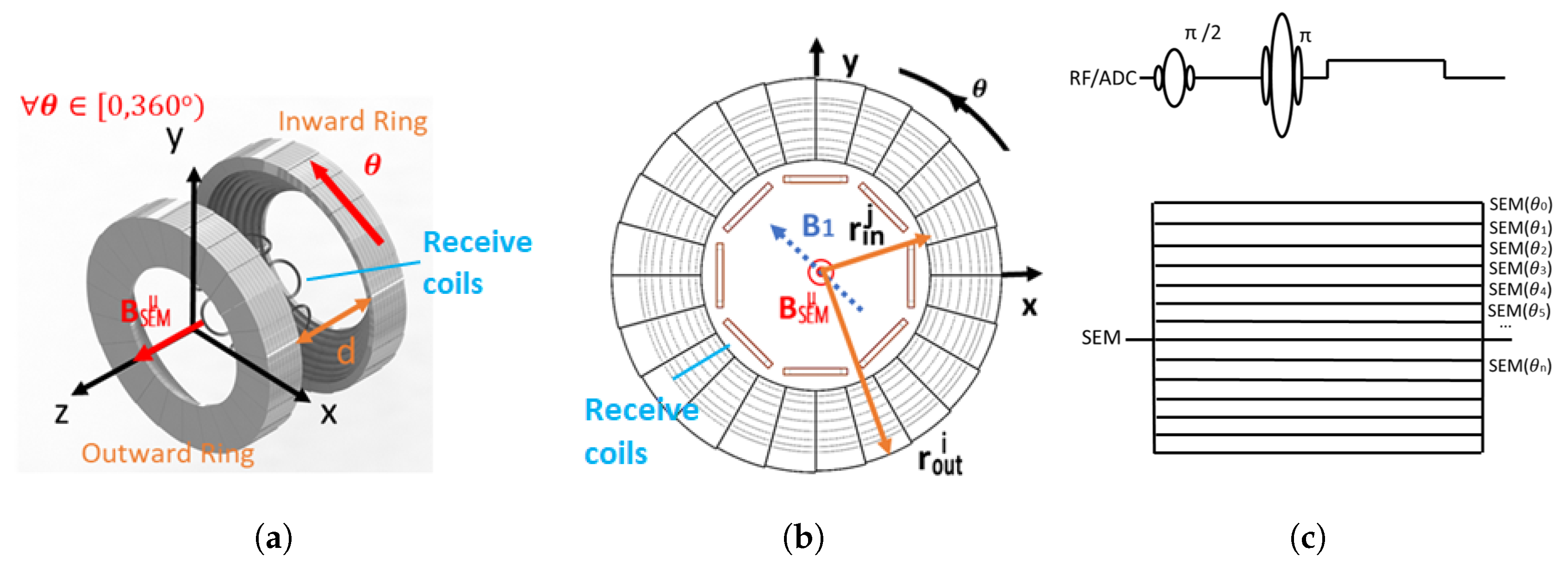
2.1. Signal Equation & Iterative Matrix Method for Image Reconstruction in a PMA-Based MRI System

In a PMB (permanent-magnet-based) MRI system, the SEM is the field that is generated by the magnet array and is used to encode the phase of the signal. When a cylindrical magnet array (e.g., an irregular inward-outward (IO) ring-pair aggregate [6] as shown in Figure 1a,b) is used, the signal equation can be expressed in Equation (1) as follows,

$$s_{\alpha }(t,\theta )={\int }_{V}m\left(\mathbf{r}\right)c_{\alpha }\left(\mathbf{r}\right)e^{-i\gamma {\int }_0^t{B}_{SEM}^{\mu }(\mathbf{r},\theta )d\tau }d\mathbf{r}$$

(1)

where t is time, $\theta$ is the angle in the $\rho –$direction on the transversal plane that defines the rotation of the cylindrical magnet array (as shown in Figure 1a,b), m is the magnetization in an object under scan, the bold letter $\mathbf{r}$ is the position vector, $c_{\alpha }$ is the sensitivity map of the ${\alpha }^{th}$ receive coil, $\gamma$ is the gyromagnetic ratio, and $B_{SEM}^{\mu }$ is the SEM generated by a magnet array at angle $\theta$. As permanent magnets are always on, $B_{SEM}^{\mu }$ inherently cannot be switched off. Figure 1c shows the pulse sequence in a PMB MRI system with a rotating cylindrical magnet array where each horizontal line represents a continuously-on SEM at angle ${\theta }_n$. In a PMB MRI system, there is less control on the SEM in time domain for image reconstruction compared to those in a PatLoc system where the SEMs are generated using coils [13,19,20]. Moreover, the pattern of the SEM is less perfect due to the imperfection of fabrication of an magnet array or/and a variation of the quality of magnets that are used to build the array. For this reason, a PMA-based system with a non-linear field is hard to be transformed to one with a linear system by mathematical tools so iterative matrix methods in time domain [3,18] are widely used in this situation.

During image reconstruction, the FoV and time are discretized by pixels. Following Equation (1), the $n_{\mathrm{t}}^{\mathrm{th}}$ sampling point of a signal at the ${n_{\theta }}^{\mathrm{th}}$ angle can be expressed using a summation as follows,

$$\begin{array}{cc}\hfill s_{\alpha }(t,\theta )=s_{\alpha }(n_t,n_{\theta })=& \sum _{n_r=1}^{N_r{N}_r}m\left(\mathbf{r}\left(n_r\right)\right)c_{\alpha }\left(\mathbf{r}\left(n_r\right)\right)e^{-i\gamma B_{SEM}^{\mu }(\mathbf{r}\left(n_r\right),(n_{\theta }\Delta \theta ))(n_t\Delta t)}\hfill \end{array}$$

(2)

where $n_{\mathrm{r}}$ is the index of the position in the FoV, $n_{\theta }$ is the index of the rotation angle ranging from 1 to $N_{\theta }$, $N_{\theta }\Delta \theta ={\theta }_{\mathrm{Max}}$ is the maximum rotation angle, $N_r{N}_r$ is the total number of pixels in the FoV, $\Delta t$ is the dwelling time, and $\Delta \theta$ is the angular step of rotation. Therefore, the image can be reconstructed by solving the following linear system,

$$\overline{s}=\overline{\overline{E}}\overline{m}$$

(3)

where $\overline{s}$ is a $N_t{N}_{\alpha }{N}_{\theta }$ column vector ($N_t$, $N_{\alpha }$, and $N_{\theta }$ are the number of the total sampling points, the number of receive coils, and the number of rotation angles, respectively), $\overline{\overline{E}}$ is a $M\times N$ encoding matrix ($M=N_t{N}_{\alpha }{N}_{\theta }$, $N=N_r{N}_r$), and $\overline{m}$ is a $N_r{N}_r$ column vector for the magnetization of the object under scan. Based on Equations (2) and (3), the entry on the nth row and the mth column of $\overline{\overline{E}}$, $e_{\mathrm{mn}}$, can be expressed using Equation (4) below,

$$e_{\mathrm{mn}}=c_{\alpha }\left(\mathbf{r}\left(n_r\right)\right)e^{-i\gamma B_{SEM}^{\mu }(\mathbf{r}\left(n_r\right),(n_{\theta }\Delta \theta ))(n_t\Delta t)}$$

(4)

which corresponds to the $\alpha$th receive coil, the $n_{\theta }^{\mathrm{th}}$ rotation angle, the $n_t^{\mathrm{th}}$ time moment, and the $n_r^{th}$ position. In Equation (4), the role of coil sensitivity ($c_{\alpha }$) and that of $B_{SEM}^{\mu }$ for signal encoding can be seen, which is to encode the amplitude and the phase of the signal, respectively.

For image reconstruction, Equation (3) in time domain can be solved by using conjugate gradient method [16] where a symmetric, positively definite matrix need to be generated. In the time domain, the conjugate of the matrix $\overline{\overline{E}}$, ${\overline{\overline{E}}}^{†}$ multiplies both sides of Equation (3), we arrive at the following equation,

$${\overline{\overline{E}}}^{†}\overline{s}={\overline{\overline{E}}}^{†}\overline{\overline{E}}\overline{m}$$

(5)

Let $\overline{b}$ = ${\overline{\overline{E}}}^{†}s$, and $\overline{\overline{A}}$ = ${\overline{\overline{E}}}^{†}\overline{\overline{E}}$, Equation (5) can be re-expressed as,

$$\overline{b}=\overline{\overline{A}}\overline{m}$$

(6)

The image can be reconstructed by solving Equation (6).

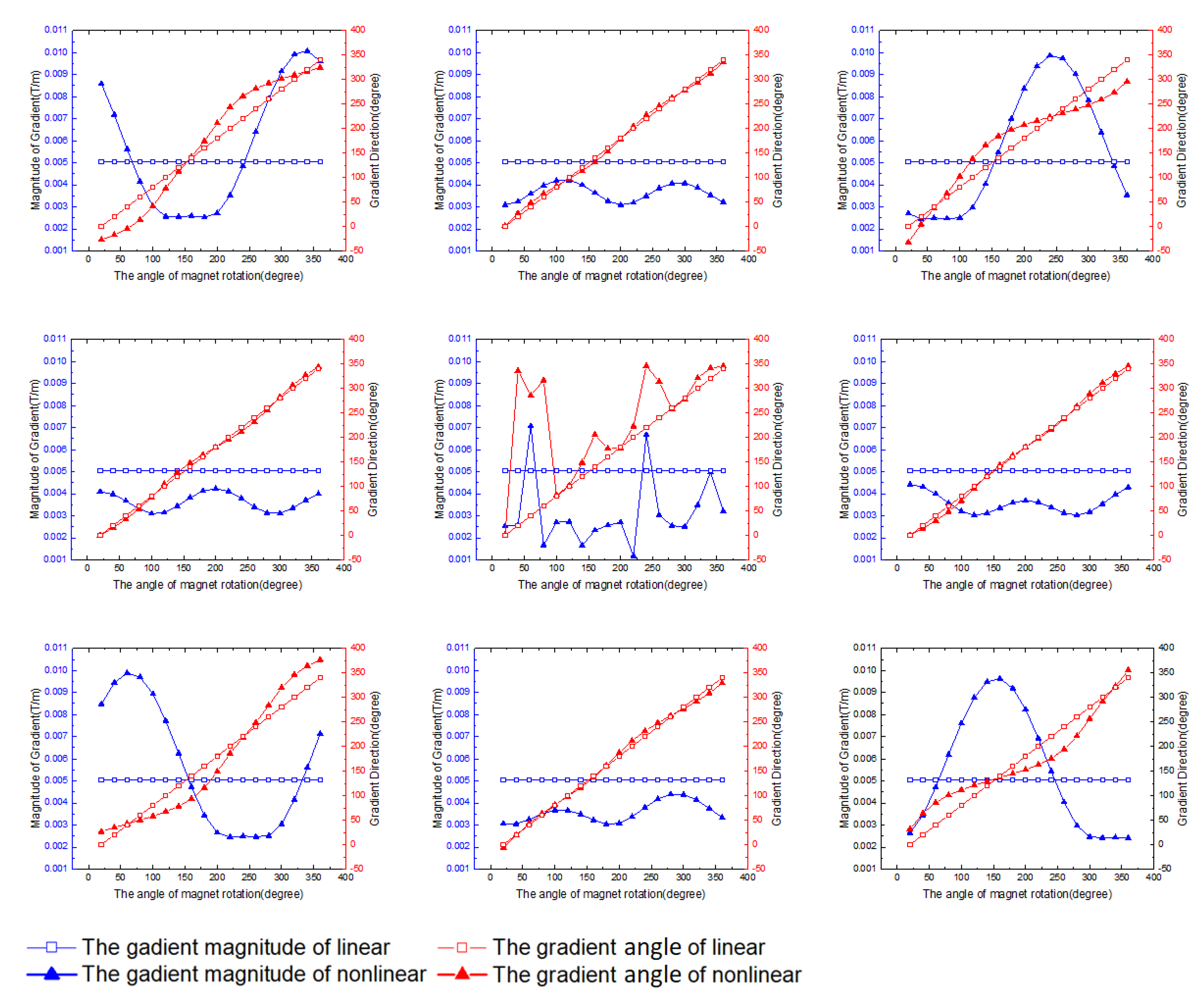
2.2. Characteristics of a Non-Linear SEM Supplied by a PMA

The SEM supplied by a permanent magnet array usually has a non-linear gradient. It is called non-linear SEM. When it is used to encode the signal in an MRI system, due to the non-linearity, a traditional k-space for the whole FoV, called a global k-space, does not provide the flexibility to interpret the system properties of regions with high-order spatial variations. Nevertheless, it has been shown in [2] that local k-spaces which are k-spaces of sub-FoVs [14,15] can be used to effectively analyze the region-dependent imaging properties of this kinds of non-linear SEMs supplied by permanent magnet arrays. Since both a global and a local k-space show distributions of acquired signals for imaging, they are called signal spaces in general in this paper.

Figure 2c,c1,c2 show the global and local k-spaces of a 2D digital phantom (with a size of FoV${}_x\times$FoV${}_y$) in Figure 2a when it is encoded by the SEMs in Figure 2b,b1 with rotations. The phantom is discretized into 21$\times$21 grids with a grid size of $\Delta x\times \Delta y$ that are labelled in Figure 2a1 (which is one of the sub-divided FoV). The linear and non-linear SEMs that have a linear and a non-linear gradient are shown in Figure 2b,b1, respectively. They have a $\Delta {\mathit{B}}_{\mathbf{0}}$ of 2 mT and an average field of 100 mT. For the non-linear SEM shown in Figure 2b1, it is supplied by a shimmed sparse IO ring-pair magnet array [21]. For an illustration, the imaging region in Figure 2a is divided into 3 × 3 sub-FoV’s for the generation of local k-spaces, and Figure 2a1 shows the sub-FoV’s at Row 2, Column 1. When Figure 2b is rotated at a step size of $\Delta \theta$ and with a total step number of $N_{\theta }$, together with a total readout time of ${\tau }_t$ and a dwelling time of $\Delta t$, Figure 2c,c1, respectively, show the corresponding global k-space and the local k-spaces located at a 3 × 3 grid that corresponds to the 3 × 3 sub-FoV’s.

In the global k-space shown in Figure 2c, the boundary of the k-space is 2$k_{\rho -max}$ × 2$k_{\rho -max}$, indicated using blue dashed line box, where $k_{\rho -max}$ is determined by the gradient of the SEM (denoted as $G_{\mathrm{SEM}}^{\mu }\left(\mathbf{r}\right)$) and the total readout time (${\tau }_t$). 2$k_{\rho -max}$ is inversely proportional to the resolution of the target image, $\Delta x$ and $\Delta y$. As shown in Figure 2c, when a linear SEM is rotated to encode the signal, the global k-space (on a global k-space coordinate system, $k_x{k}_y$-plane) has a radial pattern with a step size in the $k_{\rho }–$direction, $\Delta k_{\rho }$, and one in the $k_{\theta }–$direction, $\Delta k_{\theta }$. For the resolution of k-space, $\Delta k_{\rho }$ is determined by the size of the target image. $\Delta k_{\theta }$ is determined by the step size of the rotation, $\Delta \theta$ (Figure 1b). Here when the SEM has a linear gradient, $G_{\mathrm{SEM}}^{\mu }\left(\mathbf{r}\right)$ is a constant, $G_{\mathrm{SEM}}^{\mu }\left(\mathbf{r}\right)$ = G.

For the local k-spaces when a linear SEM is used for encoding, as shown in Figure 2c1, although they correspond to the k-spaces of the sub-FoV’s at different locations, they are identical and are identical to the global one in Figure 2c. This is because the gradient is uniform across the FoV as a result of a linear SEM. The insert in Figure 2c1 shows a zoomed-in view of the local k-space for the sub-FoV from Row 2, Column 1, on a local k-space coordinate system, $k_x^{\mathrm{loc}}{k}_y^{\mathrm{loc}}$-plane. As shown, the length and direction of the k vector in local k-space, is determined by the total readout time and the gradient of the SEM, $G_{\mathrm{SEM}}^{\mu }\left(\mathbf{r}\right)$, which is a function of location. Higher the gradient and/or longer the dwelling time, larger $\Delta k_{\rho }^{\mathrm{loc}}$ is and longer the distance between two successive signal points along the $\rho$-direction. In the case when the SEM is linear, as shown in the insert in Figure 2c1, the signal points along the $\rho$-direction is evenly distributed. For the resolution in the $\theta$-direction, $\Delta k_{\theta }^{\mathrm{loc}}$, it is determined by the rotational step of the magnet, $\Delta \theta$, and the direction of the gradient with respect to the x-axis which is set as a reference for rotation. In the case when the SEM is linear, the direction of gradient is aligned with the x-axis, which leads to that the angle of the radial line in the local k-space, ${\theta }_{ki}$, is the same as the rotation angle of the magnet. Figure 3 shows the magnitudes and angles of the gradient at the center of each FoV’s when the magnet rotates from 0° to 360° for both the linear and the non-linear SEM. As can be seen in Figure 3, when the SEM is linear, the magnitude and the angle of the gradient from each sub-FoV are identical because $G_{\mathrm{SEM}}^{\mu }\left(\mathbf{r}\right)$ is the same crossing over the FoV. This leads to an identical local k-space for each sub-FoV. Moreover, in the case when the SEM is linear, as the direction of the gradient is along the x-axis, the angles of the gradient are the same as the rotation angles of the magnet, as shown in each sub-figure in Figure 3.

When the non-linear SEM in Figure 2b1 is used for encoding, Figure 2c2 shows the 3 × 3 grid of local k-spaces. The blue dashed boxes whose sizes are determined by the linear SEM case are kept to be there as a reference. As can be seen, the k-space in each FoV is different, in terms of size, resolution, and the distribution of signal points, due to the nature of a non-linear SEM which is that the gradient is not uniform crossing the FoV, i.e., it is region dependent. This is clearly shown by Figure 3 where the magnitudes and angles of the gradients at the centers of the sub-FoVs are different from one another. When the magnitudes are large, the signal points are spread out whereas when they are small, the signal points are more concentrated within a region. Moreover, when the angle of gradient deviates away from the x-axis, the angle of the radial line in the local k-space (${\theta }_{ki}$) becomes different from the rotation angle of the magnet array. The inserts in Figure 2c2 show zoomed-in views of the local k-spaces for the sub-FoV from Row 1, Column 1 (called k-space${}_{11}$) and that from Row 2, Column 2 (called k-space${}_{22}$). As can be seen from the first insert, the signal points in k-space${}_{11}$ are much more spread out compared to the linear SEM case. They go outside the reference blue dashed box, which is due to the large magnitudes of the gradients at certain angles, as shown in the sub-figure at Row 1, Column 1 in Figure 3. The radial lines are not evenly distributed in the $\theta –$direction, which is due to the fact that the angles of the gradient deviate from the rotation angles of the magnet array. As shown in the same in sub-figure (Row 1, Column 1) in Figure 3, the deviation depends on the rotation angle. For the second insert, on the other hand, the signal points in k-space${}_{22}$ are concentrating in a small region in the box. This is because the magnitudes of the gradients are much smaller at most of the rotation angles, which is shown in the sub-figure at Row 2, Column 2 in Figure 3. For the distribution of the radial lines in the $\theta –$direction, compared to the k-space${}_{11}$, they are even more unevenly distributed, which is because the angles of the gradient deviate more from the rotation angles of the magnet array, as shown in the same sub-figure at Row 2, Column 2 in Figure 3. In the case when a non-linear SEM is used for encoding, no global k-space can represent the encoding.

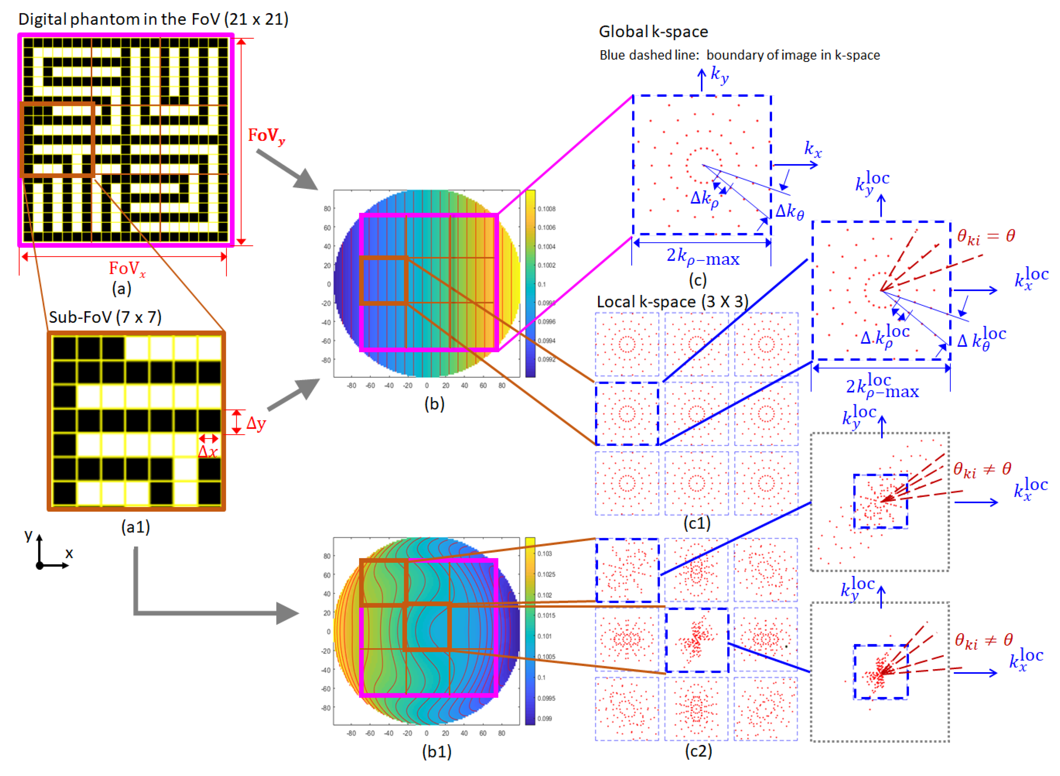
3. Investigation on the Approaches to Improve Image Quality by Increasing the Density of the Signal Space

In order to improve the image quality, a dense signal space, i.e., a dense global k-space or dense local k-spaces, are desired. For a PMA-based system, this can be obtained by increasing the number of rotation angles ($N_{\theta }$) and/or by increasing the number of sampling points ($N_t$). In this section, these two approaches are investigated and evaluated in terms of their impacts on acquisition time, image quality improvement, image reconstruction time, and memory consumption.

In terms of the effect on the signal acquisition time by taking the two approaches, in this study, the number of sampling points is increased when the total readout time is fixed. Therefore, increasing the number of sampling point does not increase the acquisition time. On the other hand, although for each radial line (i.e., each rotation angle), the maximum distance of the signal point to the origin remains the same, more sampling points can locate in the blue dashed box, especially for those cases when the gradient is high. For the second approach by increasing the number of rotation angles, it increases the density of the signal points effectively, however, the acquisition time increases proportionally with the number of the rotation angles.

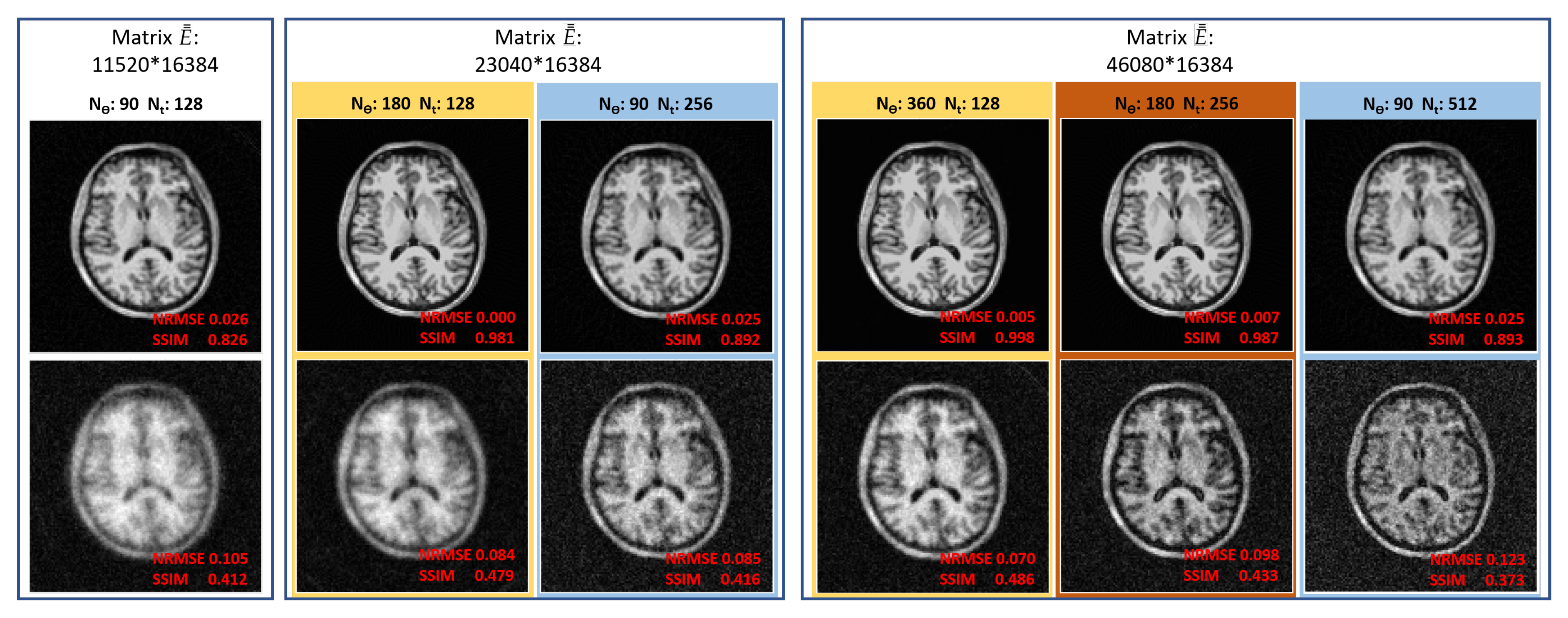
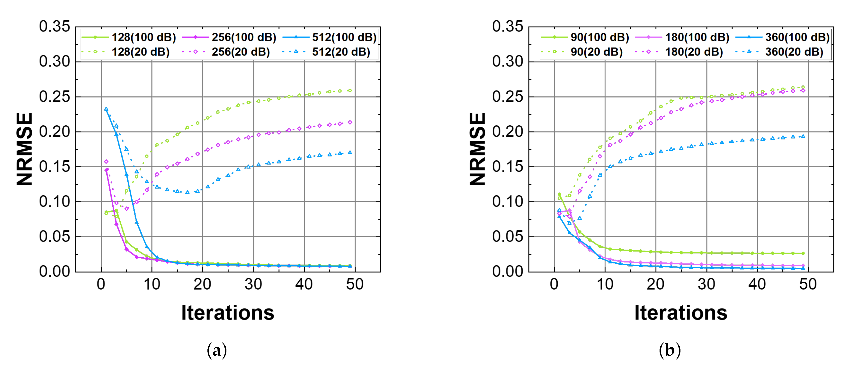
3.1. Effects on Image Quality Improvement

To investigate the effects on the image quality by taking the two approaches, i.e., increasing the number of sampling points (with a fixed total readout time) or increasing the number of rotation angles, numerical experiments were conducted. The non-linear SEM with monotonsity along the horizontal direction in Figure 2b1 were used for encoding the signal when a head phantom with a grid size of 0.78 mm was used. The sensitivity of receive coil was set to be uniform to exclude the encoding effect from the coil. The phantom was discretized into 128 × 128 and the field of view (FoV) is 100 mm × 100 mm. The SNR was set to 20 dB to mimic the situation in a low-field PMA-based system. Another case with a SNR of 100 dB was calculated for a reference. The image reconstruction in this part was conducted in the time domain where the system in Equation (6) was used. A workstation with a 256 GB RAM was used for calculation and image reconstruction. For image reconstruction, conjugate iteration method was used.

Figure 4 shows the reconstructed images. The first row shows the cases when SNR = 100 dB and the number of iterations was 10 when solving Equation (6) where the structural similarity index (SSIM) reach a maximum. The second row shows those when SNR = 20 dB and the number of iteration was 4–6 when the SSIM is the highest. The normalized root-mean-square error (NRMSE) and structural similarity index (SSIM) of each reconstructed image is labeled at the bottom in red.

In Figure 4, column 1, 3, 6 with a blue background show the reconstructed images when the number of sampling points ($N_t$) were set to 128, 256, and 512, respectively. The number of the rotation angles ($N_{\theta }$) was set to 90 and the maximum rotation angle was set to be 2$\pi$. As shown in the first row of Figure 4, at SNR = 100 dB, when $N_t$ increases from 128 to 512, the SSIM d from 0.826 to 0.893 by 8.1%. When the SNR drops to 20 dB, the reconstructed images degrade dramatically. For example at SNR = 20 dB, $N_{\theta }$ = 90, and $N_t$ = 128, as shown in the sub-figure at Row 2, Column 1 in Figure 4, most of the details in the image is too blurry to be observed. Along the same row at SNR = 20 dB, when $N_t$ increases, the central area of reconstructed image becomes clearer where the contrast increases and more details of the phantom become distinguishable and can be clearly seen. However, on the other hand, it is observed that the image quality in terms of SSIM is lowered from 0.412 to 0.373 by 9.47% with an increase in $N_t$. This is owing to the fact that by an increase in $N_t$, the noises are amplified. For this group of comparison, it can be seen that at different SNR levels, the effect and the effectiveness of improving the image quality by increasing the number of sampling points are different. At a relatively high SNR, with an increase in $N_t$, the quality of the image is improved in terms of SSIM without noticeable improvement in the details of the image that can be seen. At a relatively low SNR, with an increase in $N_t$, the details of the images becomes more distinguishable and clearer while the SSIM decreases due to an amplification of noise when more sampling points are added.

The results when the number of rotation angles increases are shown in columns 1, 2, 4 with a yellow background in Figure 4 where the number of rotation angles were set to 90, 180 and 360 and there were 128 sampling points. As shown, at SNR = 100 dB, the SSIM of the reconstructed image is improved from 0.826 to 0.998 by 20.8% with an increase in the number of rotation angles. At the same SNR, a notable improvement of image quality occurs when $N_{\theta }$ is increased from 90 to 180 where the SSIM of the corresponding image increases from 0.826 to 0.981 by 18.7%. This tendency is kept when the SNR decreases to 20 dB where the SSIM increases from 0.412 to 0.486 by 17.9%. Although the images at SNR = 20 dB are relatively blurry compared to those at SNR = 100 dB, when $N_{\theta }$ increases, the reconstructed images show more details, especially for the peripheral area, and the boundary becomes clearer. It is worth noting that the noise of the image does not increase significantly with an increase in the rotation angles degrading the image quality (i.e., lowering the SSIM), unlike the cases when the number of sampling points increases. By this comparison, increasing the number of angles shows improvement on image quality for different SNRs. At a relatively high SNR, the reconstructed image becomes clearer with an increase in $N_t$. For the cases at low SNRs, the improvement on image quality mainly is shown by clearer patterns in peripheral areas.

Both increasing $N_t$ and increasing $N_{\theta }$ show significant improvement on image quality but the behaviour is different especially when the SNR is low. In the view of the encoding matrix of the system, $\overline{\overline{A}}$ in Equation (6), both approaches help to enlarge the size of encoding matrix where more information is contained. Therefore, a further comparison of the reconstructed images is conducted when the size of the encoding matrix is the same. The second and the third blue boxes from left to right in Figure 4 show the cases when the matrix size is 23,040 ×16,384 and 46,080 ×16,384, respectively. when the SNR is high, in each box, the system with more rotation angles always gives a better image. At SNR = 100 dB, going across the boxes when the size of the matrix increases, the average SSIM increase. However, when SNR drops to 20 dB, the situation is complicated. As show in the second box where the number of rows in $\overline{\overline{A}}$ is twice of that of the original system (in the first blue box), the image of the system with more sampling points ($N_{\theta }$ = 90, $N_t$ = 256) has a high tissue contrast thus showing clearer tissue boundaries and more anatomical information. With the same matrix size and when $N_{\theta }$ is reduced and $N_t$ is increased ($N_{\theta }$ = 180, $N_t$ = 128), although the image has a high SIMM which indicate a high image quality, it is blurry where the tissue contrast is low and the tissue boundary is not clear. When the size of encoding is increased to 46,080 × 16,384, as shown in the third blue box, the system with the maximum $N_{\theta }$ ($N_{\theta }$ = 360, $N_t$ = 128) gives the highest SIMM whereas the one with the maximum sampling points ($N_{\theta }$ = 90, $N_t$ = 512) give the lowest SIMM. The later case is even worse compared to the qualities of the images when the number of rows is halved, i.e., those in the second blue box when the size of $\overline{\overline{A}}$ is 23,040 × 16,384. For the case When the system have twice of the sampling points and twice of the rotation angles ($N_{\theta }$ = 180, $N_t$ = 256) comparing to the original system (highlighted in orange background), the reconstructed image shows an improvement in image quality with a higher SIMM (an increase from 0.412 to 0.433 by 5%) and a significant enhancement of tissue contrast with a much clearer tissue boundaries.

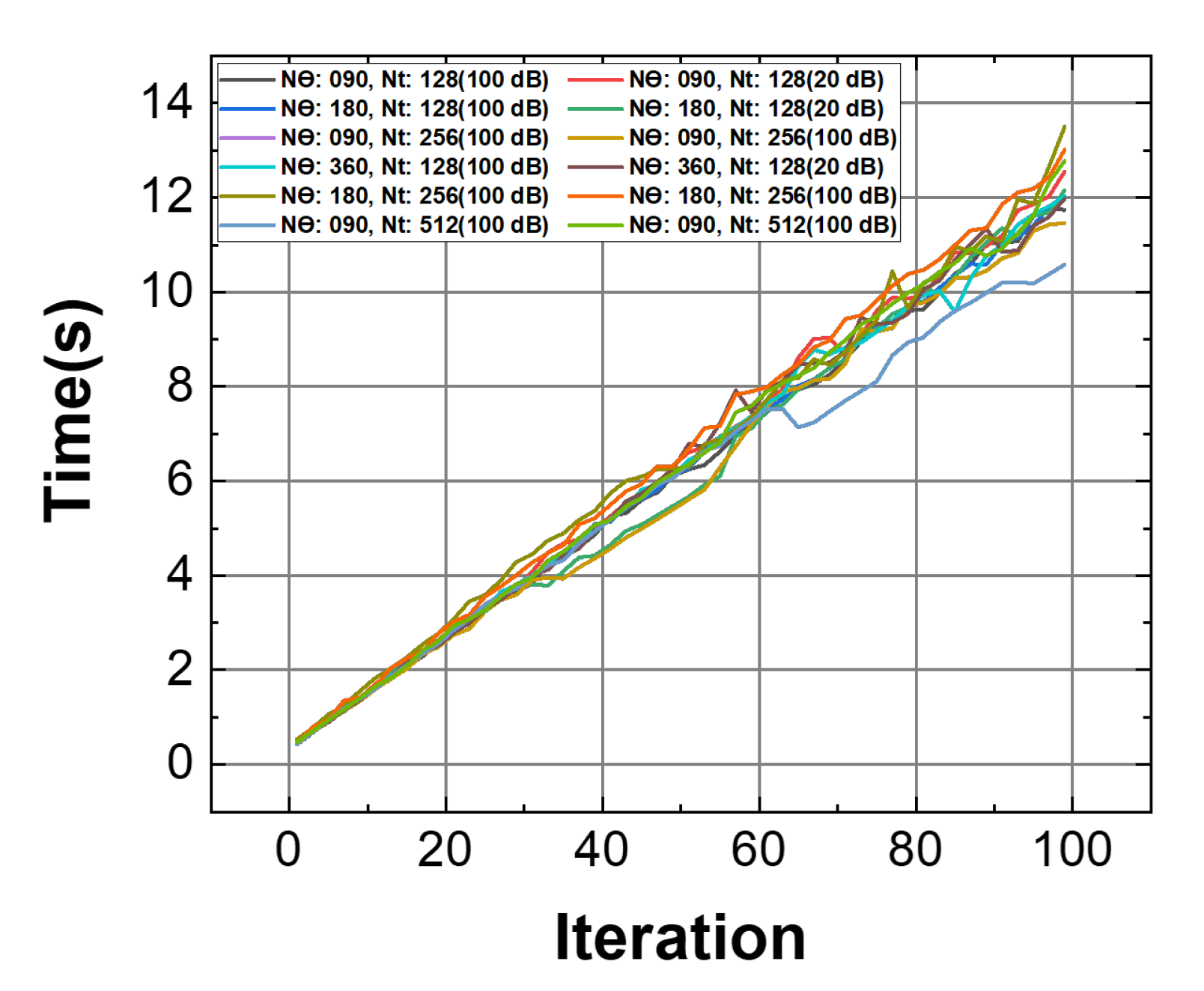
3.2. Effects on Image Reconstruction Time

In terms of image reconstruction, the system in Equation (6) is solved using conjugate gradient method [16]. As shown in Figure 4 and presented in the previous sub-section, increasing sampling points and increasing angles have different effects on image quality. To further investigate these two approaches, their effects on the image reconstruction time are examined through checking the time it takes for iterations, and the relation between the NRMSE of the solution (i.e., the resultant image) and the number of iterations.

Figure 5 shows the calculation time versus the number of iterations for the cases in Figure 4 at different $N_t$s and $N_{\theta }$s. As can be seen, the curves are all linear, close to one another, and have similar slopes. It is indicated that, although the sizes of the matrices are different, the time it takes for a single iteration is similar. The case that has the highest slope ($N_{\theta }$ = 180, $N_t$ = 256) has a computational time of 0.135 s/iteration whereas the one that has the lowest slope ($N_{\theta }$ = 180, $N_t$ = 128) has a computational time of 0.106 s/iteration.

Figure 6a shows the NRMSE of the reconstructed images versus the number of iterations when sampling points increase ($N_t$ = 128, 256, and 512, and $N_{\theta }$ = 90), corresponding to the images shown in column 1, 3, 6 in Figure 4. When the SNR is high (SNR = 100 dB), all the cases show a rapid drop of NRMSE when the number of iterations increases. At $N_t$ = 128, 256, and 512, the NRMSE drops to 0.0315, 0.0302, and 0.0299 by 71.6%, 66.8%, and 85.2% after 13 iterations compared to those of the first iteration (0.1110, 0.0911, and 0.2017), respectively. After 13 iterations, the decrease rates of all the three curves are slowed down. With the same iterations, i.e., approximately the same amount of time, the NRMSE in the case when $N_t$ = 512 decreases the fastest, changing from the highest to the lowest among the three, which indicates the highest effectiveness in terms of obtaining high image quality with the same amount of calculation time. Equivalently, it means that when $N_t$ is high, lower number of iterations, thus less computational time, leads to the same image quality. When SNR drops to 20 dB, rather than a rapid decreases and a knee-shape as those in the cases at 100 dB, each curve at this SNR shows a minimum and an increase to a saturation when the number of iterations increases. As shown, the NRMSEs at the first iteration are 0.1055, 0.1080, and 0.2070 at $N_t$ = 128, 256, and 512, respectively, which are close to the values of systems with the same $N_t$ when SNR = 100 dB. At $N_t$ = 128, unlike at 100 dB that the NRMSE decreases rapidly, the NRMSE increases when the iteration number increases. This is due to the nature of iterative method where iterations empower noise to corrupt the result [22]. When $N_t$ increases, at $N_t$ = 256 and 512, the curves show NRMSE minima of 0.0848 and 0.1108 at 3 and 9 iterations which are a decrease by 21.5% and 46.5% compared to those of the first iteration, respectively. A higher $N_t$ leads to more iterations for the system to reach a NRMSE minimum, which may be due to the fact that an increase in $N_t$ increases the size of the matrix but does not increase the information to the system proportionally. Based on the observation above, an increase in $N_t$ does not help to reduce the computational time for image reconstruction.

For the cases when $N_{\theta }$ increases (corresponding to the systems in column 1, 2, 4 in Figure 4, $N_t$ = 128, and $N_{\theta }$ = 90, 180, and 360), Figure 6b shows the relationship between the number of iterations and the resultant NRMSER. Similar to the group of systems in the previous comparison when the number of sampling points increases, the systems at 100 dB show rapid decreases in NRMSE before 15 iterations and show knee-shaped curves, and those at 20 dB have minima NRMSE and increases to saturation. The green curves show the case with $N_t$ = 128 and $N_{\theta }$ = 90 which are the same curves as the green ones in Figure 6a. At SNR = 100 dB, similar to the previous comparison, the three curves hit the saturation with the same amount of iterations (i.e., an approximately same amount of calculation time). It is noticed that the cases with a high $N_{\theta }$, $N_{\theta }$ = 180 and 360, shows a much smaller NRMSE compare to the case at $N_{\theta }$ = 90, which indicates a better image quality and agree with the observation in Figure 4. On the other hand, when SNR decrease to 20 dB, similar to the previous comparison, the NRMSEs at the first iteration in each system is similar to those at 100 dB. At $N_{\theta }$ = 180, and 360, a minimum NRMSE arrives at the third iteration at 0.0794 and 0.0696, respectively. Compared to the case at $N_{\theta }$ = 90 where the NRMSE minimal is at the first iteration, an increase in $N_{\theta }$ leads to an increase in the computational time.

For image reconstruction, conjugate gradient method was used and Equation (6) was solved where $\overline{\overline{A}}$ in Equation (6) is linked to the encoding matrix of the PMA-based MRI system as $\overline{\overline{A}}$ = ${\overline{\overline{E}}}^{†}\overline{\overline{E}}$. Matrix $\overline{\overline{A}}$ is not sparse for most of the systems, and the time consumed in each iteration is nearly same, as shown in Figure 5. At an SNR of 100 dB, based on the observations on both Figure 6a,b, all of systems need around 13–15 iterations to reach a minimal NRMSE. In the same comparison group, the number of iterations needed is the same, which is independent of the variable $N_t$ or $N_{\theta }$. This means the same amount of computational time in each group. When SNR drops and noise increases, noise corrupts the system through iterations, leading to a high NRMSE after more iterations. It is found that a noisy system with more sampling points/rotation angles requires more iterations and more time to reach the minimum NRMSE.

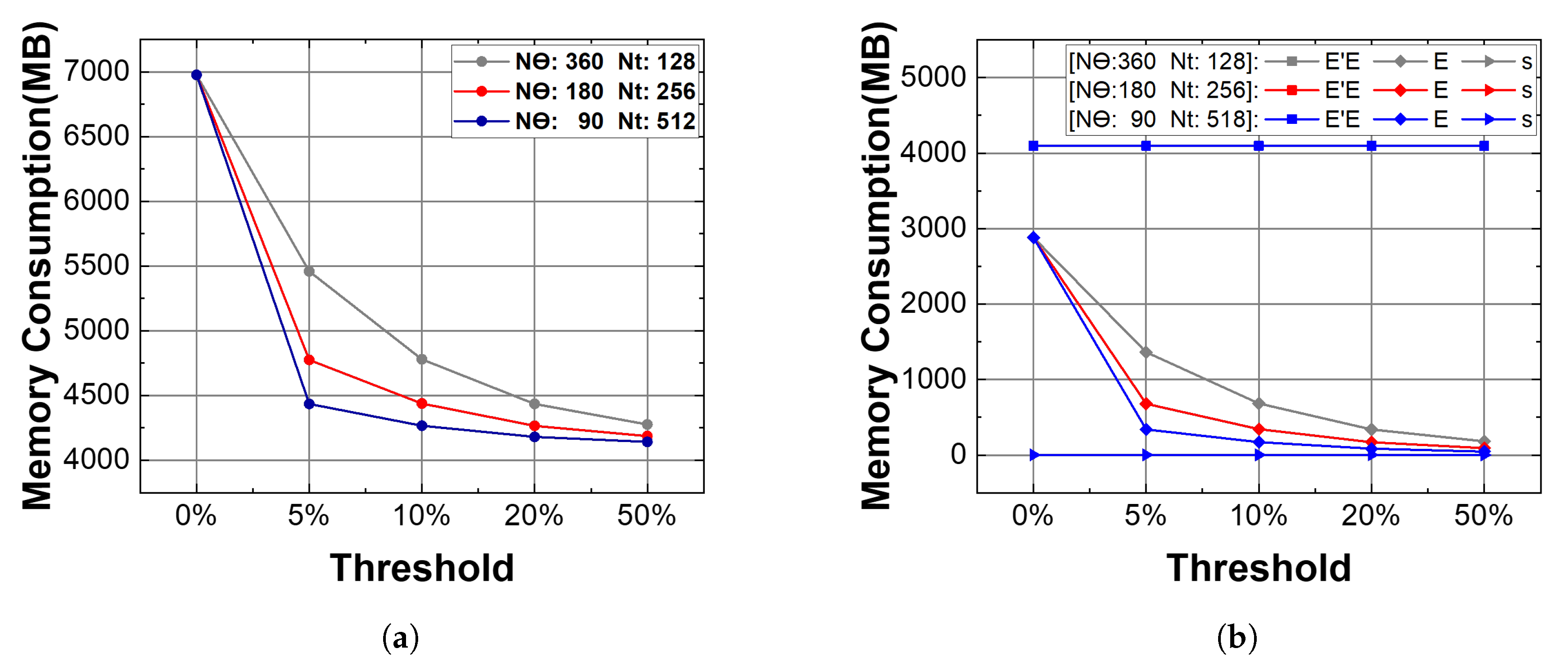
3.3. Effects on Memory Consumption

During the image reconstruction, the requirement on the memory of the computer depends on the algorithm and the size of matrix. As shown in Equation (5), the need for memory mainly comes from ${\overline{\overline{E}}}^{†}\overline{\overline{E}}$, $\overline{\overline{E}}$, and $\overline{s}$ matrix in conjugate gradient methods.

Table 1. The memory occupation in image reconstruction.

	$\overline{\overline{\mathit{A}}}$ = ${\overline{\overline{\mathit{E}}}}^{†}\overline{\overline{\mathit{E}}}$	$\overline{\overline{\mathit{E}}}$	$\overline{\mathit{s}}$	Total
$N_{\theta }$ = 90, $N_t$ = 128	4096 MB	2880 MB	0.1758 MB	6976 MB
$N_{\theta }$ = 180, $N_t$ = 128	4096 MB	5760 MB	0.3515 MB	9856 MB
$N_{\theta }$ = 90, $N_t$ = 256	4096 MB	5760 MB	0.3515 MB	9856 MB
$N_{\theta }$ = 360, $N_t$ = 128	4096 MB	11,520 MB	0.7031 MB	15,617 MB
$N_{\theta }$ = 180, $N_t$ = 256	4096 MB	11,520 MB	0.7031 MB	15,617 MB
$N_{\theta }$ = 90, $N_t$ = 512	4096 MB	11,520 MB	0.7031 MB	15,617 MB

tabulates the details of the memory consumption for each matrix in different systems. In the system in Equation (5), the size of both the encoding matrix ($\overline{\overline{E}}$) and the signal array ($\overline{s}$) increase linearly with an increase in $N_{\theta }$ and $N_t$. In terms of the memory consumption, as shown in the table, those consumed by $\overline{\overline{E}}$, $\overline{s}$, and the total memory increase with an increment in $N_t$ and/or $N_{\theta }$. When $N_t$ is increased from 128 to 512 when $N_{\theta }$ = 90, The memory consumed by $\overline{\overline{E}}$ increases from 2880 MB to 11,520 MB, that by $\overline{s}$ increases from 0.1758 MB to 0.7031 MB, and the total memory increases from 6976 MB to 15,617 MB. On the other hand, it is noticed that ${\overline{\overline{E}}}^{†}\overline{\overline{E}}$ has a fixed memory consumption (4096 MB) while that of $\overline{\overline{E}}$ increases from 2880 MB to 11,520 MB.

For the encoding matrix $\overline{\overline{E}}$, as indicated by the expression of its entry in Equation (4), the row number of $\overline{\overline{E}}$ is decided by the number of sampling points ($N_t$), rotation angles ($N_{\theta }$) and receive coils ($N_{\alpha }$) meanwhile the column number of $\overline{\overline{E}}$ always equal to the number of pixels in the target image ($N_r{N}_r$). Therefore, when $N_t$ or $N_{\theta }$ increases, the memory consumption of $\overline{\overline{E}}$ increases linearly with them, as can be seen in Table 1. On the other hand, the Hermite positive semi-definite matrix, $\overline{\overline{A}}$ = ${\overline{\overline{E}}}^{†}\overline{\overline{E}}$, has a size fixed at $N_r{N}_r\times N_r{N}_r$. Therefore, the memory consumption does not increase with an increase in either the number of sampling point or the number of rotation angles. As shown in Table 1, the increase in the total memory required is mainly caused by an increase in the memory of the encoding matrix.

To improve the image quality in a PMA-based system, it has been shown that increasing $N_t$ or/and $N_{\theta }$ are effective approaches. However, taking this approach can considerably higher the memory required for image reconstruction, which makes it difficult to be handled by a handheld computer. In the example when $N_t$ increases from 128 to 512 when $N_{\theta }$ = 90 shown in Table 1, the memory requirement increases from around 7 GB to more than 14 GB, which is easily doubled. In reality, to obtain good image quality by increasing the number of sampling points or rotation angles, denser sampling points are needed and the required memory can easily go beyond the memory of a normal laptop (e.g., 64 GB). Therefore, image reconstruction that requires memory that can be handled by a portable computer is crucial. In the next section, we make the encoding matrix sparse for a memory-saving image reconstruction in such a PMA-based MRI system.

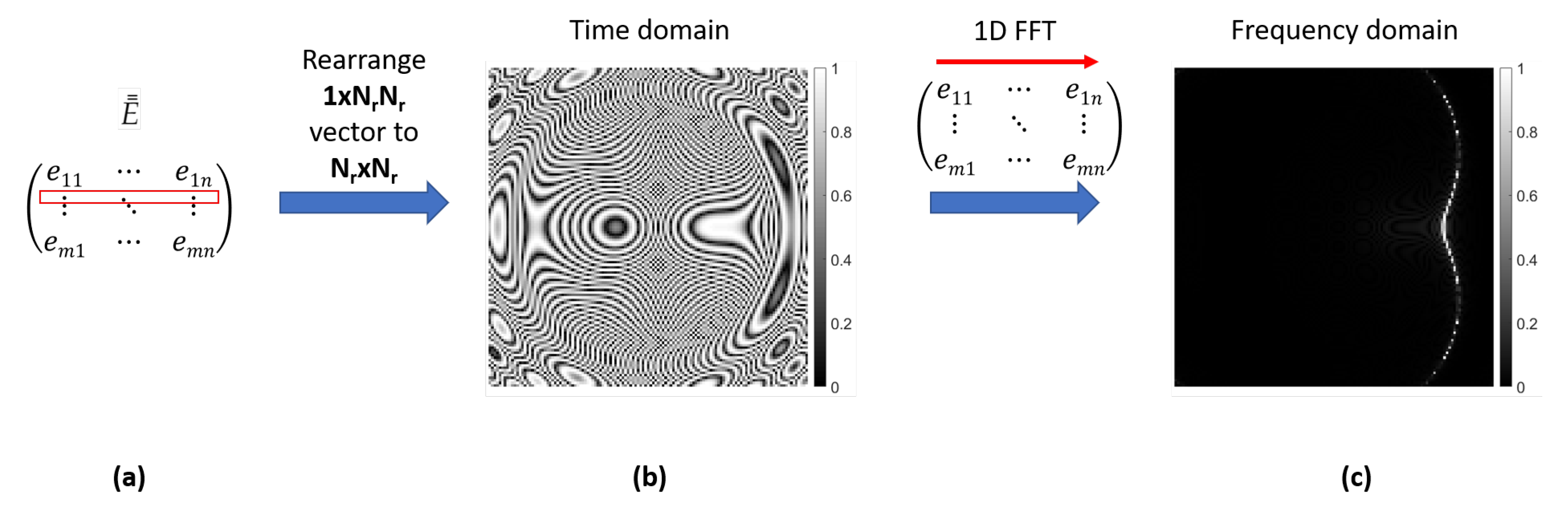
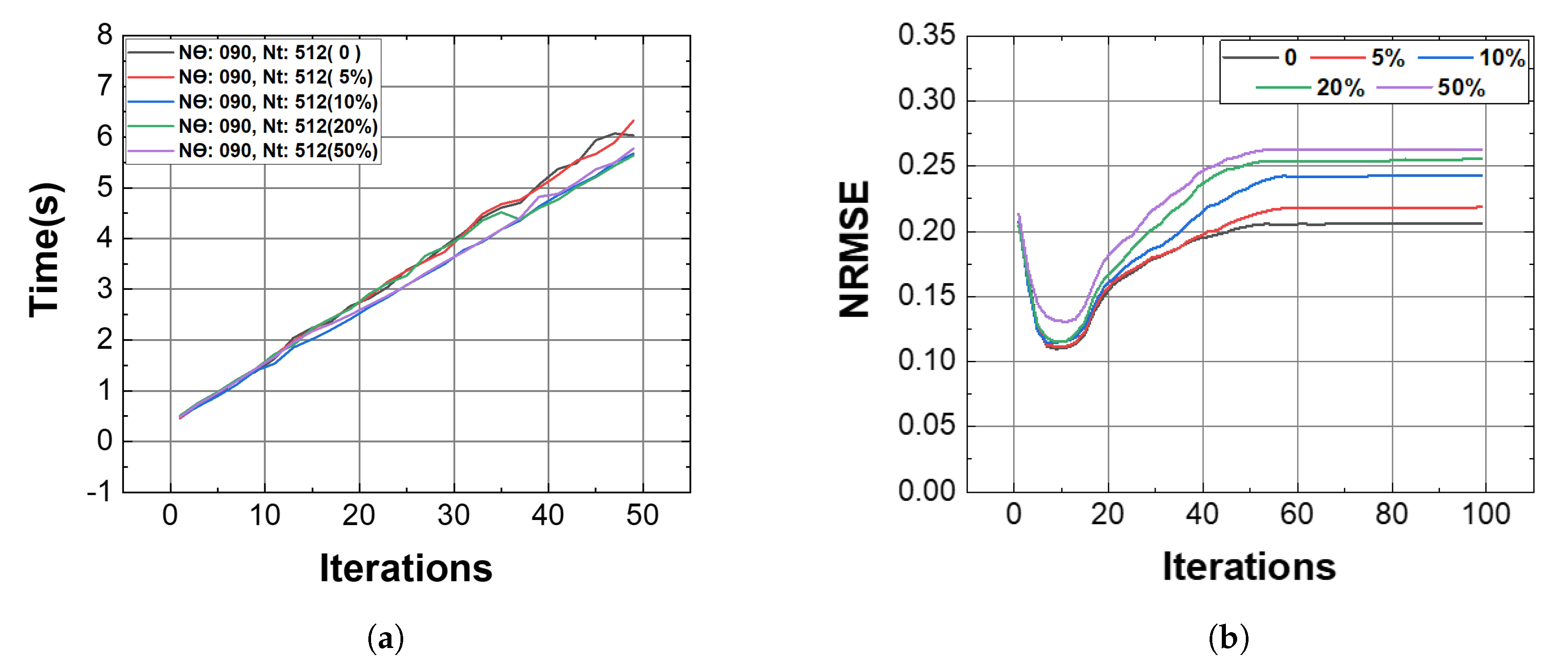
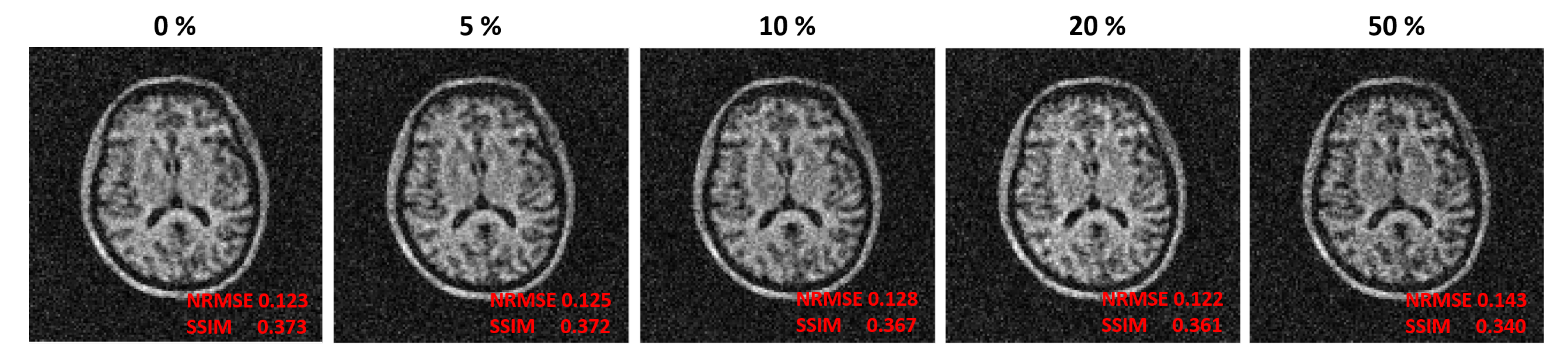
4. The Memory-Saving Reconstruction

To make the encoding matrix sparse, it can be done by transforming the matrix from time domain to frequency domain by 1D fast Fourier transfer (FFT) [15,17]. Figure 7 shows an illustration of the transformation. As shown in Figure 7a, each element in each row in $\overline{\overline{E}}$ (time domain) contains the encoding information of each image pixel. By doing the FFT along the readout direction, as shown in Figure 7c, the distribution of the row in the resultant matrix in frequency domain concentrates in a much smaller area (Figure 7d) rather than widely spread out in time domain (Figure 7b), which makes the matrix in frequency domain much sparser than that in time domain. For the plots in time domain and in frequency domain as shown in Figure 7b,d, respectively, the data from the first row of the encoding matrices were used. The non-linear SEM in Figure 2b1 was used with a total rotation angle number ($N_{\theta }$) of 72, the maximum rotation angle (${\theta }_{\mathrm{Max}}$) of 2$\pi$, and a number of the total sampling points ($N_t$) of 256. As shown in Figure 7, in the time domain, most of the entries of the encoding matrix contribute to the signal point equally, whereas in the frequency domain, only the entries from a narrow area (the bright curve) have countable contributions to the signal point.

By doing FFT for the signal array and the encoding matrix, Equation (7) is rewritten as below,

$$DFT\left(\overline{s}\right)=DFT(\overline{\overline{E}})\overline{m}$$

(7)

where the 1D FFT of $\overline{\overline{E}}$ in Equation (3) is column-wise. Let $DFT(\overline{s})$ = $\overline{f}$, $DFT(\overline{\overline{E}})$ = ${\overline{\overline{E}}}_f$, Equation (7) can be re-written as following,

$$\overline{f}={\overline{\overline{E}}}_f\overline{m}$$

(8)

Solving Equation (8) gives the same reconstructed image as that by solving Equation (3) yet the encoding matrix in Equation (8) is much more sparse than that in Equation (3). The transformation results in a much sparser matrix for image reconstruction, which will lead to a reduction in the memory that is required.

Furthermore, to further reduce the memory consumption during the image reconstruct, for the sparse encoding matrix in the frequency domain in Equation (8), the entries that are relatively small are zeroed/truncated. A row-wise truncation of the encoding matrix is used where the truncation is conducted based on the maximum value of the entries of each row. The row-wise truncation further reduces the memory slightly compared to a global one [17] where the global truncation is used as a reference value for a truncation. Denote the row-wise threshold in percentage as $t{h}_{\mathrm{r}-\mathrm{w}}$, Equation (8) can be re-expressed as,

$$\overline{f}={\overline{\overline{E}}}_{f-t{h}_{\mathrm{r}-\mathrm{w}}}\overline{m}$$

(9)

where ${\overline{\overline{E}}}_{f-t{h}_{\mathrm{r}-\mathrm{w}}}$ is the encoding matrix after the row-wise truncation. In ${\overline{\overline{E}}}_{f-t{h}_{\mathrm{r}-\mathrm{w}}}$, the entries in each row are zeroed when they are less than $t{h}_{\mathrm{r}-\mathrm{w}}$ percent of the maximum values of the entries in that row.

Table 2. The memory occupation in image reconstruction ($N_{\theta }$ = 90, $N_t$ = 512).

Threshold	$\overline{\overline{\mathit{A}}}$ = ${\overline{\overline{\mathit{E}}}}^{†}\overline{\overline{\mathit{E}}}$	$\overline{\overline{\mathit{E}}}$	$\overline{\mathit{s}}$	Total
0	4096 MB	11,520 MB	0.7 MB	15,617 MB
5%	4096 MB	338.8 MB	0.7 MB	4436 MB
10%	4096 MB	170.7 MB	0.7 MB	4267 MB
20%	4096 MB	84.5 MB	0.7 MB	4181 MB
50%	4096 MB	45.1 MB	0.7 MB	4142 MB

shows the memory consumption of the system with $N_{\theta }$ = 90 and $N_t$ = 512 when the image reconstruction was conducted in the frequency domain. As shown in Table 2, when the threshold was set at 5%, the total memory for calculation was reduced from 15,617 MB to 4436 MB by 71.6%. When this threshold increases, the total memory drops further, i.e., a further reduction of 294 MB when the threshold increases from 5% to 50%. It is noticed that the decrease rate in memory slow down when the threshold is more than 5%. The reason is that although the memory consumed by the encoding matrix can be reduced significantly by the truncation, the matrix $\overline{\overline{A}}$, remains dense, which leads to a constant memory consumption for this matrix. Matrix $\overline{\overline{A}}$ dominates the memory consumption when the truncation percentage is high and its memory consumption saturates the total required memory.

Figure 8a,b respectively show the total memory consumption and the individual ones versus the truncation percentage for the three systems that has a matrix size of 46,080 × 16,384 when $N_{\theta }$ = 90 and $N_t$ = 512, $N_{\theta }$ = 180 and $N_t$ = 128, and $N_{\theta }$ = 180 and $N_t$ = 256. As shown in Figure 8a, the three cases show similar trends where the total memory consumption drops dramatically when the truncation threshold is 5%, at least 10,000 MB of memory is saved, and slows down when the truncation percentage further increases. This is for the same reason mentioned previously for the case with $N_{\theta }$ = 90 and $N_t$ = 512 that the memory consumption for the encoding matrix ($\overline{\overline{E}}$) decreases with an increase in the truncation percentage while that for matrix $\overline{\overline{A}}$ and the vector array $\overline{s}$ stay the same, as shown in Figure 8b, where the memory for matrix $\overline{\overline{A}}$ is relatively high and saturates the total memory consumption when the truncation percentage is high. For the decrease in the memory consumption of the encoding matrix, it is observed that the system that has a high $N_{\theta }$ requires more memory under the same threshold (>0) when the size of $\overline{\overline{E}}$ is the same. Considering the effects of the truncation on the calculation time, image quality, the memory consumption, 5% truncation has the best balance among the three performances.

In terms of the effect of the truncation on the computational time and image quality, Figure 9a,b show the calculation time and the NRMSE of the images versus the number of iterations for the systems when $N_{\theta }$ = 90 and $N_t$ = 512. The SNR was set at 20 dB. As shown in Figure 9a, the curves are close to one another, and the computational time of all the systems has a linear relation with the number of iterations, which indicates that the calculation time for each iteration is the same and the effect of the truncation is negligible. In terms of the number of iterations it takes to arrive at a NRMSE minimum, all the systems show an iteration number of about 10, which implies a similar amount of calculation time for the system to have the best image quality. Comparing the curves, it is noticed that the 50%-truncation case has the highest minimum NRMSE, which can be reflected in the reconstructed images. Figure 10 shows the reconstructed images of each case when their NRMSE is minimum. The corresponding NRMSEs and SSIMs are labelled in each image. As can be seen, as the truncation percentage increases, the features become blurry, the NRMSE increases, and the SSIM decreases.

5. Conclusions

This study investigates the approaches for image quality improvement in a PMA-based MRI system, and proposes an effective approach to obtain both a memory-saving reconstruction and a significant improvement in image quality simultaneously in such a system. An IO-ring PMA was used as an example to supply a non-linear SEM with non-linear gradients. Local k-spaces were used to identify the problem caused by non-linear gradients to the quality of reconstructed images which is the uneven population of signal points in the local k-spaces. To tackle this problem, increasing sampling points and increasing rotation angles are both investigated and their effectiveness was examined and demonstrated through numerical examples. The downside of this remedy was then clearly identified which is an significant increase in the memory consumption due to a resultant large and dense encoding matrix. To cut down the memory consumption after the size of the encoding matrix is increased through increasing the sampling points or rotation angles, the resultant large and dense matrix is transformed to the Fourier domain (frequency domain) where the matrix becomes sparse and the memory consumption is significantly reduced. The efficacy of the memory reduction was successfully shown. A truncation was proposed on the sparse encoding matrix in the frequency domain to further reduce the memory consumption. The effects of truncation with different percentage on the total memory consumption, the calculation speed, and the quality of reconstructed images were investigated where optimal truncation was identified with a good balance on the trade-offs.

According to the investigation, increasing the sampling points leads to a stronger tissue contrast while increasing the number of rotation angles leads to clearer tissue boundaries. An increase in the memory consumption caused by an increase in the sampling points and rotation angles is successfully and effectively lowered down by a transformation of the system to frequency domain. Consequently, a system with a large matrix for a pursue of an improved quality of the image construction can be handled by a laptop. The proposed study is one step forward for a PMA-based MRI system towards its targeted point-of-care application scenario.

References

1. Huang, S.Y.; Ren, Z.H.; Obruchkov, S.; Gong, J.; Dykstra, R.; Yu, W. Portable Low-cost MRI System based on Permanent Magnets/Magnet Arrays. Investig. Magn. Resonance Imaging (iMRI) 2019, 23, 179–201. [Google Scholar] [CrossRef]
2. Gong, J.; Huang, S.Y.; Ren, Z.H.; Yu, W. Effects of Encoding Fields of Permanent Magnet Arrays on Image Quality in Low-field Portable MRI Systems. IEEE Access 2019, 7, 80310–80327. [Google Scholar] [CrossRef]
3. Cooley, C.Z.; Stockmann, J.P.; Armstrong, B.D.; Sarracanie, M.; Lev, M.H.; Rosen, M.S.; Wald, L.L. Two-dimensional imaging in a lightweight portable MRI scanner without gradient coils. Magn. Resonance Med. 2015, 73, 872–883. [Google Scholar] [CrossRef] [Green Version]
4. Ren, Z.H.; Maréchal, L.; Luo, W.; Su, J.; Huang, S.Y. Magnet array for a portable magnetic resonance imaging system. In Proceedings of the 2015 IEEE MTT-S 2015 International Microwave Workshop Series on RF and Wireless Technologies for Biomedical and Healthcare Applications (IMWS-BIO), Taipei, Taiwan, 21–23 September 2015; pp. 92–95. [Google Scholar]
5. Ren, Z.H.; Mu, W.C.; Huang, S.Y. Design and optimization of a ring-pair permanent magnet array for head imaging in a low-field portable mri system. IEEE Trans. Magn. 2019, 55, 1–8. [Google Scholar] [CrossRef]
6. Ren, Z.H.; Gong, J.; Huang, S.Y. An Irregular-shaped Ring-Pair Magnet Array with a Monotonic Field Gradient for 2D Head Imaging in Low-field Portable MRI. IEEE Access 2019. [Google Scholar] [CrossRef]
7. Esparza-Coss, E.; Cole, D.M. A low cost MRI permanent magnet prototype. AIP Conf. Proc. 1998, 440, 119–129. [Google Scholar]
8. Rokitta, M.; Rommel, E.; Zimmermann, U.; Haase, A. Portable nuclear magnetic resonance imaging system. Rev. Sci. Instrum. 2000, 71, 4257–4262. [Google Scholar] [CrossRef]
9. Kimura, T.; Geya, Y.; Terada, Y.; Kose, K.; Haishi, T.; Gemma, H.; Sekozawa, Y. Development of a mobile magnetic resonance imaging system for outdoor tree measurements. Rev. Sci. Instrum. 2011, 82, 053704. [Google Scholar] [CrossRef] [PubMed] [Green Version]
10. Nakagomi, M.; Kajiwara, M.; Matsuzaki, J.; Tanabe, K.; Hoshiai, S.; Okamoto, Y.; Terada, Y. Development of a small car-mounted magnetic resonance imaging system for human elbows using a 0.2 T permanent magnet. J. Magn. Resonance 2019, 304, 1–6. [Google Scholar] [CrossRef] [PubMed]
11. Eidmann, G.; Savelsberg, R.; Blümler, P.; Blümich, B. The NMR MOUSE, a mobile universal surface explorer. J. Magn. Reson. 1996, 122, 104–109. [Google Scholar] [CrossRef]
12. Cooley, C.Z.; Haskell, M.W.; Cauley, S.F.; Sappo, C.; Lapierre, C.D.; Ha, C.G.; Stockmann, J.P.; Wald, L.L. Design of sparse Halbach magnet arrays for portable MRI using a genetic algorithm. IEEE Trans. Magn. 2017, 54, 1–12. [Google Scholar] [CrossRef] [PubMed]
13. Hennig, J.; Welz, A.M.; Schultz, G.; Korvink, J.; Liu, Z.; Speck, O.; Zaitsev, M. Parallel imaging in non-bijective, curvilinear magnetic field gradients: A concept study. Magn. Resonance Mater. Phys. Biol. Med. 2008, 21, 5. [Google Scholar] [CrossRef] [PubMed] [Green Version]
14. Gallichan, D.; Cocosco, C.A.; Dewdney, A.; Schultz, G.; Welz, A.; Hennig, J.; Zaitsev, M. Simultaneously driven linear and nonlinear spatial encoding fields in MRI. Magn. Resonance Med. 2011, 65, 702–714. [Google Scholar] [CrossRef] [PubMed]
15. Gallichan, D.; Cocosco, C.A.; Schultz, G.; Weber, H.; Welz, A.M.; Hennig, J.; Zaitsev, M. Practical considerations for in vivo MRI with higher dimensional spatial encoding. Magn. Resonance Mater. Phys. Biol. Med. 2012, 25, 419–431. [Google Scholar] [CrossRef] [PubMed] [Green Version]
16. Lin, F.H.; Witzel, T.; Schultz, G.; Gallichan, D.; Kuo, W.J.; Wang, F.N.; Hennig, J.; Zaitsev, M.; Belliveau, J.W. Reconstruction of MRI data encoded by multiple nonbijective curvilinear magnetic fields. Magn. Resonance Med. 2012, 68, 1145–1156. [Google Scholar] [CrossRef] [Green Version]
17. Schultz, G.; Gallichan, D.; Reisert, M.; Hennig, J.; Zaitsev, M. MR image reconstruction from generalized projections. Magn. Resonance Med. 2014, 72, 546–557. [Google Scholar] [CrossRef]
18. Stockmann, J.P.; Ciris, P.A.; Galiana, G.; Tam, L.; Constable, R.T. O-space imaging: Highly efficient parallel imaging using second-order nonlinear fields as encoding gradients with no phase encoding. Magn. Resonance Med. 2010, 64, 447–456. [Google Scholar] [CrossRef] [Green Version]
19. Schultz, G.; Ullmann, P.; Lehr, H.; Welz, A.M.; Hennig, J.; Zaitsev, M. Reconstruction of MRI data encoded with arbitrarily shaped, curvilinear, nonbijective magnetic fields. Magn. Resonance Med. 2010, 64, 1390–1403. [Google Scholar] [CrossRef]
20. Schultz, G.; Weber, H.; Gallichan, D.; Witschey, W.R.; Welz, A.M.; Cocosco, C.A.; Hennig, J.; Zaitsev, M. Radial imaging with multipolar magnetic encoding fields. IEEE Trans. Med Imaging 2011, 30, 2134–2145. [Google Scholar] [CrossRef]
21. Mu, W.C.; Gong, J.; Ren, Z.H.; Yu, W.; Huang, S.Y. Sparse Inward-outward (IO) Ring-Pair Permanent Magnet Array (PMA) with a Light Rotation Load for Low-field Head Portable MRI. Preprint 2019. [Google Scholar] [CrossRef]
22. De Leeuw den Bouter, M.L.; van Gijzen, M.B.; Remis, R.F. Conjugate gradient variants for p-regularized image reconstruction in low-field MRI. SN Appl. Sci. 2019, 1, 1736. [Google Scholar] [CrossRef] [Green Version]
Figure 1. An irregular inward-outward ring-pair aggregate proposed in [6] (a) 3D view, (b) front view, (c) Pulse Sequence.
Applsci 10 02177 g001
Figure 2. A 2D digital phantom and its global and local k-spaces when spatial encoding magnetic (SEM) with linear and non-linear gradients are used for signal encoding.
Applsci 10 02177 g002
Figure 3. The magnitudes and angles of gradients at the center of each sub-FoV when the magnet rotates from 0° to 360° for both the linear and the non-linear SEM in Figure 2b,b1, respectively.
Applsci 10 02177 g003
Figure 4. The reconstructed images of brain phantom (a grid size of 0.78125 mm, a discretization of 128 × 128, a FoV of 100 mm × 100 mm) in numerical simulation when the non-linear SEM in Figure 2b1 was used. The SNRs of the first and the second rows correspond to the encoding at 100 dB and 20 dB, respectively. Different columns corresponds to the encoding with different numbers of rotation angles and different numbers of sampling points which is labeled on the top of first row. The systems with same size of E ¯ ¯ are organized in the blue box. The original phantom is collected by a 3T conventional MRI system.
Applsci 10 02177 g004
Figure 5. The relationship between time and iterations in different systems.
Applsci 10 02177 g005
Figure 6. The relationship between image quality and iteration under conjugate gradient reconstruction (a) the number of sampling point changed in the system with 90 angles. (b) the number of angle changed in the system with 128 sampling points.
Applsci 10 02177 g006
Figure 7. The sequence of memory-saving method on the encoding matrix E ¯ ¯ in time domain. (a) the encoding matrix E ¯ ¯ in time domain; (b) a 2D plot of one 1 × N r N r row in E ¯ ¯ re-arranged into a N r × N r matrix in time domain; (c) a 2D plot of one 1 × N r N r row in E ¯ ¯ after it is converted to frequency domain using 1D FFT and re-arranged into a N r × N r matrix in frequency domain.
Applsci 10 02177 g007
Figure 8. The memory consumption versus the truncation percentage at different N θ and N t . (a) the total memory consumption (b) the memory consumption for each parameters.
Applsci 10 02177 g008
Figure 9. The system in Equation (9) with N θ = 90 and N t = 512 (a) the relationship between time and the number of iterations, (b) the relation between normalized root-mean-square error (NRMSE) and the number of iterations.
Applsci 10 02177 g009
Figure 10. The reconstructed images of a human head phantom (a grid size of 0.78125 mm, a discretization of 128 × 128, a FoV of 100 mm × 100 mm) when the non-linear SEM in Figure 2b1 was used. N θ = 90, N t = 512, and the SNRs was set to be 20 dB. The truncation percentages were set to be 0%, 5%, 10%, 20%, and 50%.
Applsci 10 02177 g010