A Deep Learning-Based Method to Detect Components from Scanned Structural Drawings for Reconstructing 3D Models

Abstract

Among various building information model (BIM) reconstruction methods for existing building, image-based method can identify building components from scanned as-built drawings and has won great attention due to its lower cost, less professional operators and better reconstruction performance. However, this kind of method will cost a great deal of time to design and extract features. Moreover, the manually extracted features have poor robustness and contain less non-geometric information. In order to solve this problem, this paper proposes a deep learning-based method to detect building components from scanned 2D drawings. Taking structural drawings as an example, in this article, 1500 images of structural drawings were firstly collected and preprocessed to guarantee the quality of data. After that, the neural network model—You Only Look Once (YOLO) was trained, verified and tested. In addition, a series of metrics were utilized to evaluate the performance of recognition. The results of test experiments show that the components in structural drawings (e.g., grid reference, column and beam) can be successfully detected, while the average detection accuracy of the whole image is over 80% and the average detection time for each image is 0.71 s. The experimental results demonstrate that the proposed method is robust and timesaving, which provides a good basis for the reconstruction of BIM from 2D drawings.

1. Introduction

In recent years, more and more practical cases [1,2,3] have verified the promotion of BIM technology in operation and maintenance (O&M) management of buildings. The application of BIM technology can guarantee the information passing from construction phase to O&M phase and help owners or managers to make better decisions on O&M activities, such as fault diagnosis, facilities management, space management, data monitoring, energy consumption analysis, and emergency evacuation, based on more accurate and comprehensive information [4]. However, most of the existing buildings are currently designed and built based on 2D drawings due to their long history [5], which results in the lack of building information models. Therefore, how to quickly, accurately and cost-effectively reconstruct 3D models of existing buildings has become the focus of research work in this field.

Numerous techniques and methods have been proposed to build effective and reliable building information models for existing buildings. For example, photogrammetry [6] can obtain building information (e.g., shape, size and position of building) and build 3D models by processing the building image, which is acquired by optical camera, but this type of model only contains geometric and physical information, while the precision for single building is lower compared to other methods. Laser scanning [7] can efficiently create 3D models of existing buildings through point clouds, however, it is invalid when dealing with the components hidden above ceilings or behind walls [8]. In addition, the cost of using laser scanning devices is relatively high [1]. Other methods like reconstructing 3D models based on 2D vector drawings [9] can extract not only geometrical information but also topological and semantic information of buildings. The downside of this method is that there are a number of drafting errors [10,11] in CAD drawings, which will definitely have a bad effect on the precision of reconstruction models. Moreover, a large proportion of existing buildings have been built for more than 20 years, so instead of CAD vector drawings, only paper-based drawings or hand-drawn blueprints may remain [12].

Different from the methods mentioned above, the method that scans CAD drawings or hand-drawn blueprints into digital formats and extracts information from those raster images using image processing technique [5] has received more attention from researchers due to its high efficiency, low cost and widespread applicability. As the first step of an image-based method, component recognition plays a significant role in reconstructing BIM for existing buildings. Traditionally, geometric primitives (lines, polylines, arcs, etc.) obtained by feature extraction are combined into building components based on predefined definitions about geometric constraints and topological relations [13]. However, components may be represented in different ways due to the diversity of drawing standards and drawing conventions in different countries [9]. As a result, the traditional component recognition approach, which predefines the rules, cannot satisfy all kinds of expressions. Therefore, a smarter method that can be widely applied to various conditions is needed to identify building components from raster images of CAD drawings [14].

In this paper, a novel method that automatically detects structural components from scanned CAD drawings was proposed based on a convolutional neural network called You Only Look Once (YOLO). The reasons for choosing structural components as research objects are listed as follows: (1) the continuous occurrence of decoration, refurbishment and reconstruction project during O&M phase may lead to a marked change of existing buildings, especially for the components in the architecture and mechanical system, and (2) structural framings (e.g., columns, beams and shear walls) are hardly changed since they are the most fundamental and significant part of the entire building. Hence, the actual condition of structural components will be consistent with those shown in structural CAD drawings.

2. Literature Review

2.1. Traditional Methods for Components Recognition

The general process to identify building components based on the raster image of the CAD drawing can be divided into two steps: primitive recognition and building element recognition [5].

The primitive recognition identifies basic geometric primitives (e.g., lines, arcs and circles) from the images of CAD drawings using image processing techniques and computer vision techniques. The essence of this step is feature extraction, which determines whether each pixel in the image belongs to a feature and extracts core information (e.g., shape, color, texture, spatial relations or text) based on these image features. Numerous feature extraction algorithms, like Hough Transform [15], scale invariant feature transform (SIFT) [16], maximally stable extremal regions (MSER) [17], and speeded-up robust features (SURF) [18], have been proposed in the past few decades for different tasks of object recognition. Among these algorithms, Hough Transform is one of the most common and significant methods to recognize geometric primitives from raster images of CAD drawing. More than 2500 papers focus on its improved algorithms and applications [19]. Some improved algorithms have been developed based on classical Hough Transform, such as Generalized Hough Transform [20], Progressive Probabilistic Hough Transform [21], Random Hough Transform [22], Digital Hough Transform [23], and Fuzzy Hough Transform [24].

After identifying geometric primitives, the next step, namely building element recognition, mainly defines several classification rules based on geometric constraints and topological relations, and categorizes these geometric primitives according to pre-established rules. Many researchers have been working on the recognition of building components in architectural floor plan for a long time [25]. Macé et al. [26] proposed a method to detect walls based on the distance and texture between the parallel lines. Ahmed et al. [27] distinguished walls from other components by dividing the lines into three levels: thick, medium, and thin. Riedinger et al. [28] took the binarization process for the floor plan first, then the main walls and the dividing walls were detected and located based on the thickness of dark sketches, which represent wall seams. Grimenez et al. [9] identified building components like walls, doors, windows, and rooms from floor plans using the method of pattern recognition. Meanwhile, others focus on the recognition of structural components in 2D drawings. Lu et al. [29] put forward a shape-based method to detect parallel pairs (PPs) of structural elements like shear walls and bearing beams. Moreover, Lu et al. [30] divided the whole image of structural drawing into several segments through detecting the symbol of grids, and then the location information of columns, beams and slabs were extracted with the help of Optical Character Recognition (OCR) technology. Instead of dealing with structural components, Cho et al. [8] payed more attention to the 2D mechanical drawings and developed an algorithm with a relatively high accuracy to extract the geometrical information of mechanical entities such as ducts, elbows, branches and pipes as well as their corresponding semantic information.

Although existing component recognition methods can be used to identify specific components from CAD drawings, a major disadvantage of these methods is that it spends a lot of time to manually design and extract features, and the robustness of the features extracted in these conventional methods is poor. In addition, since the components obtained from existing methods are composed of several geometric primitives or symbols defined by the fixed pre-established regulations, the generalization ability is weak when dealing with the same components represented in different standards or drawn with different design conventions. Therefore, it is necessary and valuable to propose a more intelligent method to identify structural components in different types of structural CAD drawings. Due to the higher accuracy, strong generalization ability, simple operation, and lower cost (unnecessary to buy expensive measuring instruments), the deep learning technology was performed to detect components in this paper. Moreover, deep learning-based object detection method has been successfully applied in other fields of civil engineering [31,32,33], but no researches using this method were found to identify components in CAD drawings, especially for structural components. The development of deep learning methods in object detection will be reviewed in following section.

2.2. Deep Learning Methods for Object Detection

In recent years, deep learning is one of the research hotspots in the field of artificial intelligence. The rationale of deep learning is to make a computer learn to simulate the way of thinking in the human brain as well as the transmission mode of signal in nervous systems. At present, deep learning has made breakthroughs in object detection such as gesture detection [34], iris detection [35], license plate detection [36], face detection [37], and human action detection [38]. According to the process of detection, deep learning algorithms can be divided into two categories: two-stage object detection algorithm and one-stage object detection algorithm.

The two-stage object detection algorithm converts the object detection problem into a classification problem. The overall process can be divided into two stages. First, the region proposal is generated, and then the classifier is utilized to classify and amend the region proposal. Ross Girshick et al. firstly proposed Region-Based Convolutional Neural Network (R-CNN) [39] by using a selective search [40]. However, this algorithm requires a large amount of time to calculate and detection speed is slow. To improve R-CNN, Girshick developed Fast Region-Based Convolutional Neural Network (Fast R-CNN) [41] based on the idea of Spatial Pyramid Pooling Layer (SPP) [42]. Fast R-CNN greatly improves the speed of detection since it only performs convolution calculation once for the whole image. However, the process of a selective search for generating a region proposal in Fast R-CNN run on the CPU, still spends so much time on convolution calculation. Based on Fast R-CNN, Ren et al. put forward a new algorithm, namely Faster Region-Based Convolutional Neural Network (Faster R-CNN) [43], to merge the generation of region proposal and the classification of CNN together and take all the computation with the help of GPU. As a result, there is a significant increase in speed as well as accuracy. He et al. [44] proposed Mask R-CNN based on Faster R-CNN for object detection and instance segmentation. A limitation of this algorithm is that the cost of labeling when segmenting the instance is too expensive. Moreover, its detection speed still cannot reach the real-time level.

The essence of one-stage object detection approach is to transform the object detection problem into a regression problem. Different from the process in the two-stage algorithm that generates the region proposal first, one-stage object detection algorithm can directly create the class probability and coordinate information of the target object through the CNN, which immensely improves the efficiency of objection detection and meets the requirements of real-time detection in computing speed. Redmon et al. [45] proposed an algorithm named YOLO through dividing an image into N×N grids and predicting the two bounding boxes and their corresponding category information for each grid. On the basis of YOLO, Liu et al. [46] came up with the SSD based on the anchor mechanism of Faster R-CNN, which guarantees the high accuracy as well as the fast speed of the detection. However, the effect for recognizing a small target is not particularly desirable. To address these problems, researchers proposed some improved algorithms based on YOLO. The YOLOv2 [47] was developed to improve the detection accuracy and speed by adding batch normalization, multi-scale training and anchor box after each convolutional layer. The YOLO9000 [47] combined the ImageNet dataset [48] and the COCO dataset [49] together and achieved the detection of 9418 kinds of objects using the method of WordTree hierarchical classification.

2.3. Selection for Structural Component Detection

As shown in Section 2.2, when the accuracy meets certain baselines, deep learning approaches are continuously developed for the speed of detection. Besides, in some application scenarios of object detection, it is noted that researchers prefer to use deep learning algorithms with a simple structure and faster detection speed. In particular, YOLO and improved algorithms based on YOLO are widely applied. YOLO is an end-to-end model that directly predicts the location of bounding boxes and the class probabilities of objects from the original image. Due to this concise and straightforward detection process, the detection speed of YOLO is extremely fast and the object in video can be detected in real-time. Meanwhile, comparing the two-stage object detection approaches like R-CNN, Fast R-CNN and Faster R-CNN, YOLO has less background errors since it trains on the whole image, which effectively helps to acquire contexture information about the target object. In addition, YOLO has characteristics of quick convergence and strong generalization ability.

Furthermore, structural components such as beams and columns in structural drawings have several characteristics like small size, high similarity and less features. When detecting these components using a deep learning-based method, a deep convolutional neural network is needed to form more abstract features to represent the location and category information. Moreover, a structural drawing always contains hundreds of components, and there are dozens of such drawings in a construction project. As a result, the detection method is needed to meet the precision for object detection as well as the speed nearly up to real-time level.

Therefore, according to the analysis mentioned above, YOLO is recommended to use for detecting structural components in scanned CAD drawings.

3. Methodology

Figure 1 illustrates the overall process of proposed YOLO-based component detection method. First of all, the images of 2D structural drawings are collected and classified into five classes: grid reference, column, horizontal beam, vertical beam, and sloped beam. Then a series of image processing operations are performed to decrease the noises and improve the quality of images for the following detection step. After image preprocessing, dataset management is carried out to label and augment image data. Next, images in an augmented dataset are utilized to train YOLO, and the test set is applied to evaluate the detection performance of structural components. Finally, the detection results are output to a file in TXT format, which includes information about the classification and localization of components. The following provides a detailed explanation for the main steps in the proposed method.

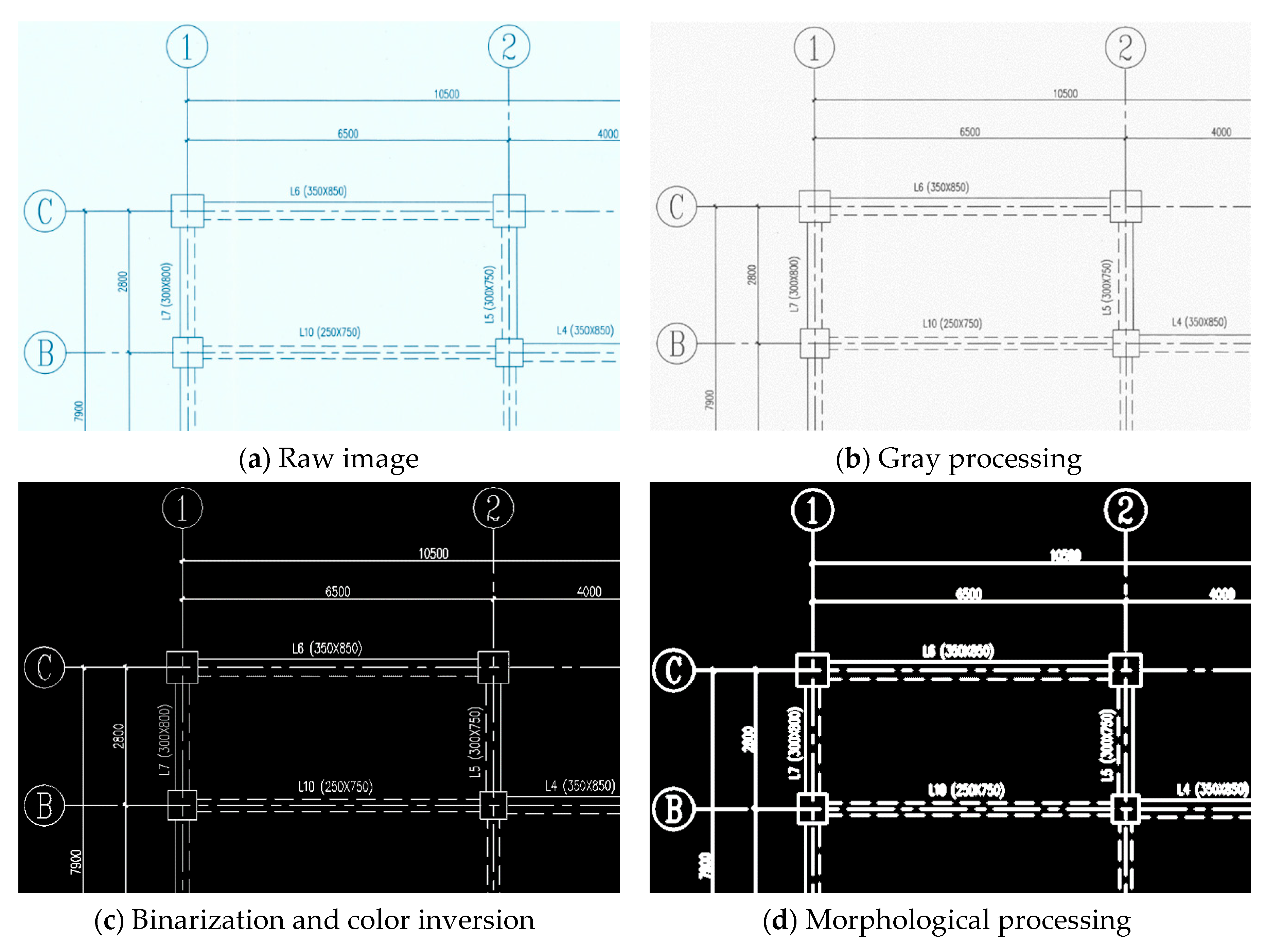
3.1. Image Preprocessing

It can be seen in Figure 2a that components in structural drawing images mainly have two characteristics: (1) a single component only occupies a small proportion of the entire image, and (2) these structural components, which are generally composed of lines or arcs, do not differ significantly from each other. As a result, most of structural components in 2D drawings lack strong and distinctive features. Besides, since the images utilized in this study are generated by scanning paper drawings, noises would be produced during this process, which may have a bad effect on the performance of detection. In addition, the images of scanned structural drawings normally contain three image channels of red, green and blue. Training YOLO through these raw images directly without any processing will result in a large amount of computational consumption. To overcome these problems, a series of image preprocessing steps are carried out to reduce the data amount and improve images quality used in subsequent detection steps. The main processes include: gray processing, binarization and color inversion, and morphological operation.

3.1.1. Gray Processing

Gray processing is used to convert color images into grayscale images. In RGB color mode, the color of each pixel is co-determined by the R, G, and B components and each component may take a value between 0 and 255. When R = G = B, the resulting color is a gray color, and the value of R = B = G is called grayscale value. At this time, only 1 byte is needed for each pixel to store the grayscale value. Same as the value range of the three components, the grayscale value of each pixel varies from 0 to 255 and represents the different intensity of light. In general, image gray processing includes three common-used methods [50]: average method, weighted average method and maximum method. In this paper, the weighted average method is utilized to calculate the grayscale value for each pixel according to Equation (1). The effect of gray processing for the structural drawing image is shown in Figure 2b.

F = 0.2989R + 0.5870G + 0.1140B,

(1)

3.1.2. Binarization and Color Inversion

Binarization is the process of setting the grayscale value of pixels to 0 or 255, so that the image only shows black or white color. The mathematical expression of this process is shown as follows:

$$G\left(x,\mathrm{y}\right)=\{\begin{array}{ll}255& f\left(x,y\right)\ge T\\ 0& f\left(x,y\right)<T\end{array},$$

(2)

where f (x, y) represents the original grayscale value of a pixel in structural drawing image, T is the threshold value, and G (x, y) denotes the grayscale value of a pixel after binarization. If the grayscale value f (x, y) is smaller than a given threshold T, the grayscale value of this pixel is set to 0; otherwise, the value changes to 255.

Furthermore, Color inversion is performed once the grayscale image has been converted into a binary image. If the original grayscale value of a pixel is 255, its grayscale value is reset to 0. Otherwise, the grayscale value is reset to 255.

The processes of image binarization and color inversion further reduce the amount of data in the image as well as the interference of background. Consequently, features of structural components will be highlighted. The effect of binarization and color inversion for a structural drawing image is shown in Figure 2c.

3.1.3. Morphological Operation

The aforementioned steps have reduced the data size and alleviate the influence of image background on final detection performance. However, features of components themselves are still weak since lines or arcs that normally make up a structural component in drawings are thin. This has become the main question in this step.

To address this issue, a morphological processing technology called dilation was applied to deal with the semi-finished images of structural drawings. Dilation expands the white part of the image so that the new image has larger bright regions. In other words, structural components in images will be thicker than before. It is assumed that A is an image of structural drawings to be processed, and B is the core used to dilate A. The dilation equation is defined as follows [51]:

$$A\oplus B=\cup \left\{A+b:b\in B\right\},$$

(3)

where $\oplus$ represents dilation operation.

The final image after dilation is shown in Figure 2d. Dilation makes it easier for YOLO to extract features from scanned structural drawings and thus improves the performance of component detection. Furthermore, semantic information corresponding to the structural components in the images is also dilated, which promotes the robustness of subsequent extraction of semantic information from 2D structural drawings by using Optical Character Recognition (OCR) technique.

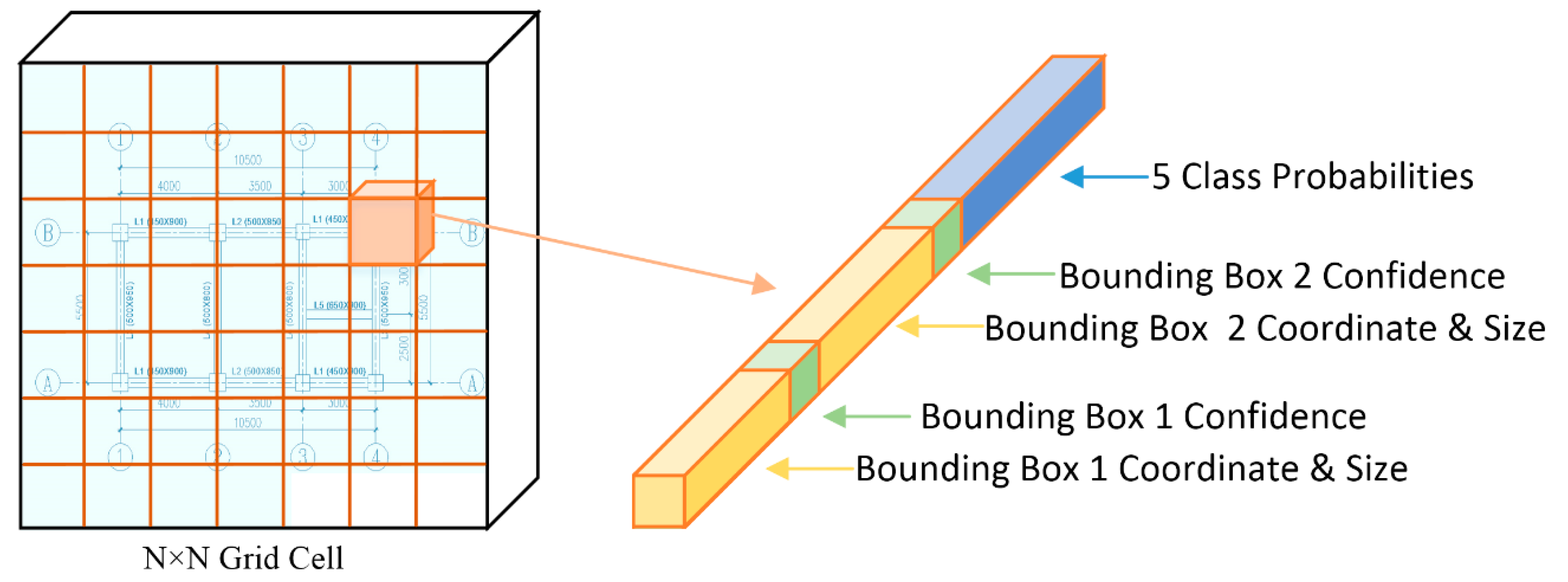
3.2. YOLO for Structural Components Detection

When YOLO is utilized to detect components in 2D structural drawings, images of these drawings are input and divided into N × N grids firstly, and then each grid cell is responsible for three types of predictions (as shown in Figure 3): (1) pixel coordinates and size of two bounding boxes, (2) confidence of two bounding boxes, and (3) the probabilities that a cell contained five classes of components. Finally, these predictions are output as a N × N × (5 × 2 + 5) tensor.

3.2.1. Architecture of YOLO

As shown in

Table 1. Architecture of YOLO.

Layer	Name	Filter	Kernel Size/ Stride	Layer	Name	Filter	Kernel Size/ Stride
0	Covn.1	64	7 × 7 / 2	15	Conv.13	256	1 × 1 / 1
1	Maxp.1	/	2 × 2 / 2	16	Covn.14	512	3 × 3 / 1
2	Covn.2	192	3 × 3 / 1	17	Covn.15	512	1 × 1 / 1
3	Maxp.2	/	2 × 2 / 2	18	Covn.16	1024	3 × 3 / 1
4	Covn.3	128	1 × 1 / 1	19	Maxp.4	/	2 × 2 / 2
5	Covn.4	256	3 × 3 / 1	20	Covn.17	512	1 × 1 / 1
6	Covn.5	256	1 × 1 / 1	21	Covn.18	1024	3 × 3 / 1
7	Covn.6	512	3 × 3 / 1	22	Covn.19	512	1 × 1 / 1
8	Maxp.3	/	2 × 2 / 2	23	Covn.20	1024	3 × 3 / 1
9	Covn.7	256	1 × 1 / 1	24	Covn.21	1024	3 × 3 / 1
10	Covn.8	512	3 × 3 / 1	25	Covn.22	1024	3 × 3 / 2
11	Covn.9	256	1 × 1 / 1	26	Covn.23	1024	3 × 3 / 1
12	Covn.10	512	3 × 3 / 1	27	Covn.24	1024	3 × 3 / 1
13	Covn.11	256	1 × 1 / 1	28	Conn.1	/	/
14	Covn.12	512	3 × 3 / 1	29	Conn.2	/	/

, the neural network of YOLO used in this paper has 24 convolution layers with different core sizes and two fully connected layers, and the max-pooling technique is applied to extract the main characteristics as well as to reduce the computational complexity [45].

Convolution layer: The purpose of convolutional layers is to extract features from structural drawing images by convolving the input data with convolutional cores of fixed size and to produce feature maps as an output. According to Table 1, the convolutional layers of YOLO in this paper include 3 × 3 and 1 × 1 convolutional cores. The 3 × 3 convolutional cores are used for convolution, while the 1 × 1 cores are used to reduce the number of input channels, decrease the parameters generated in the neural network, and lighten the computation burden when training YOLO.

Max-pooling layer: The max-pooling layer segments the feature map according to the spatial position of the feature matrix in the feature map. The maximum value obtained from each segment area is then used as a new eigenvalue. Table 1 reveals that the filter of max pooling in this paper is 2 × 2 with stride 2. It means that the maximum values, taken respectively in each segment area, with 2 strides, will be as the new eigenvalue, and the new feature map is generated based on these eigenvalues. After max-pooling operation, the new feature map is reduced by four times while the important information is remained in the former feature map. In addition, the image is abstracted to a higher level, which allows the following convolutional layers to extract features from it at multiple scales.

Fully connected layer: The fully connected layer mainly deals with the dimensionality reduction problem, which turns the input 2D feature matrices into feature vectors, to facilitate the prediction and classification of structural components in the output layer. In the neural network of YOLO, two fully connected layers are connected to the feature map, which has undergone the process of convolution and max pooling to generate an output tensor.

Moreover, in order to increase the nonlinearity of each layer of the neural network in YOLO, a linear activation function is applied for the final fully connected layer, while the leaky rectified linear activation function [45] is utilized for the rest of the layers and is shown as:

$$\varnothing \left(x\right)=\{\begin{array}{ll}x,& x>0\\ 0.1x& x\le 0\end{array},$$

(4)

3.2.2. Loss Function

In order to keep a balance among coordinate predictions, category predictions and confidence predictions when training YOLO, an improved sum-squared error (SSE) method [45] is applied in this study to optimize the loss function. The specific loss function is shown as follows:

$$\begin{array}{l}{\lambda }_{\mathrm{coord}}{\displaystyle {\displaystyle \sum }_{i=0}^{S^2}}{\displaystyle {\displaystyle \sum }_{j=0}^B}{1}_{ij}^{\mathrm{obj}}[{(x_i-{\widehat{x}}_i)}^2+\left(y_i-{\widehat{y}}_i{)}^2\right]\\ +{\lambda }_{\mathrm{coord}}{\displaystyle {\displaystyle \sum }_{i=0}^{S^2}}{\displaystyle {\displaystyle \sum }_{j=0}^B}{1}_{ij}^{\mathrm{obj}}[{(\sqrt{w_i}-\sqrt{{\widehat{w}}_i})}^2+(\sqrt{h_i}-\sqrt{{\widehat{h}}_i}{)}^2]\\ +{\displaystyle {\displaystyle \sum }_{i=0}^{S^2}}{\displaystyle {\displaystyle \sum }_{j=0}^B}{1}_{ij}^{\mathrm{obj}}{(C_i-{\widehat{C}}_i)}^2\\ +{\lambda }_{\mathrm{noobj}}{\displaystyle {\displaystyle \sum }_{i=0}^{S^2}}{\displaystyle {\displaystyle \sum }_{j=0}^B}{1}_{ij}^{\mathrm{noobj}}{(C_i-{\widehat{C}}_i)}^2\\ +{\displaystyle {\displaystyle \sum }_{i=0}^{S^2}}{1}_i^{\mathrm{obj}}{\displaystyle {\displaystyle \sum }_{c\in classes}}{(p_i\left(c\right)-{\widehat{p}}_i\left(c\right))}^2,\end{array}$$

(5)

where ${\lambda }_{\mathrm{coord}}$ denotes the weight of the localization error while ${\lambda }_{\mathrm{noobj}}$ is the weight of the classification error when the bounding box contain no objects. $(x,y,w,h)$ reveals pixel coordinate information and size information of the target’s bounding box appearing in grid i, and $(\widehat{x},\widehat{y},\widehat{w},\widehat{h})$ represents the same information for the actual object in grid i. $1_i^{\mathrm{obj}}$ indicates that there is an object in the j^th bounding box of the grid i, while $1_{ij}^{\mathrm{noobj}}$ means no object exists in the same bounding box. B denotes the number of bounding boxes predicted in each grid, and S² grid denotes the number of grids partitioned by the input image. $C_i$ is a component class predicted by grid i, and ${\widehat{C}}_i$ is the actual class of the component in the image.

There are five parts in Equation (5), the first two parts denote the localization error about the center coordinate and the width and height of the bounding box. The third part calculates the loss of confidence of the bounding box containing objects, while the fourth part obtains the loss without objects. The final part represents the conditional probability error for the class of objects.

3.3. Detection Result Export

According to Section 3.1, it can be seen that each grid cell predicts five probabilities and two candidate bounding boxes. To acquire the most possible class and its corresponding bounding box from the grid cell, non-maximal suppression (NMS) algorithm [52] is applied. NMS algorithm suppresses non-maximal elements and acts as a local maximum search. As a result, the bounding box with the highest class-specific confidence score will be extracted.

However, since the detection results obtained above are generated in the code, they cannot be utilized directly following researches of semantic information matching and BIM model reconstruction of existing buildings. Moreover, some of the data in detection results like the width and height of bounding box are useless in the subsequent study, applying these results without any change will result in an increase of output. Therefore, to optimize the output data, a file in txt format is exported in this study to record the detection results of structural components. As shown in Figure 4, four types of information are required to contain in this txt file: component ID, class of detection, pixel coordinate, and confidence of bounding box.

4. Experiment and Results

4.1. Data Preparation

To identify structural components from 2D drawings, a large number of images with class labels are necessary to train and test the YOLO model. However, there is no public and general-purpose image dataset of structural drawings with multiple labeled classes in the field of object detection so far. Therefore, this study collected and established a dataset consisting of 500 images of 2D structural drawing with a fixed resolution of 850 × 750. Two types of structural drawing images were included in this dataset: the column layout plan image (CLPI) and the framing plan image (FPI). Each image was obtained by scanning a paper-based structural drawing. The components to be recognized in the image were divided into five classes: grid reference, column, horizontal beam, vertical beam, and sloped beam. Here grid reference refers to the corresponding numbers of grids, and the reason for regarding the grid reference as one of the structural components is that the successful recognition of the grid reference will be beneficial to the establishment of component coordinate systems in the future, which plays a significant role in matching the topological and semantic information of structural components. Moreover, the names of three types of beams are used to represent the different placement directions of them on 2D structural drawings. For example, if a beam spans horizontally, it will be regarded as a horizontal beam. Otherwise it will be considered as a vertical beam or sloped beam.

4.1.1. Image Labeling

Once images in the dataset had been completed all the operations of image preprocessing mentioned above, the structural components in the images were labeled based on their classes. In this paper, LabelImg [53] was used to label the scanned 2D drawings. The components to be annotated were selected with a box respectively, and then tags were assigned to the corresponding boxes. Finally, the labeled images were output as XML format. To increase the features of structural components, which have a significant influence on the final results of detection, when boxing the components, the semantic information corresponding to the components was also selected. Taking beam as an example, correct and incorrect labeling on the image of the structural drawing are shown in Figure 5.

4.1.2. Data Augmentation

Based on Section 3.2.1, it can be inferred that the neural network of YOLO used in this study has a multi-layer structure that contains millions of parameters. To make these parameters work well, a great deal of data is needed to be trained. Otherwise, overfitting may occur during the training process and then there will be a poor performance of component detection on the new image. Therefore, to avoid the overfitting problem when training on a small dataset and improving the generalization ability of the YOLO model, image augmentation technique was implemented in this study to increase the size of the dataset by randomly cropping and translating images in the original dataset. A total of 1000 new images were generated in this phase, and all original and newly generated images were mixed together to form an augmented dataset. After that, this augmented dataset was used for training and testing to prevent classification bias in the process of structural component detection.

4.2. Experiment Design

4.2.1. Experiment Environment and Strategy

The experiment was carried out on a PC with a processor of Intel Core (TM) i7-6700, RAM of 32 GB and GPU of NVIDIA GeForce GTX 1080 Ti. In addition, Python 2.7.15 was utilized as programming language on the operating system of Ubuntu 16.04, and structural component detection was performed using the deep-learning framework of Tensorflow-gpu 1.1.0. Moreover, CUDA 8.0 was applied to make GPU acceleration, and OpenCV [54] was used for image pre-processing and image visualization during the process of training and testing.

When training YOLO in this article, a weight decay of 0.0005 was applied, and 0.9 for the momentum. Moreover, epoch and batch size were manually set to 160 and 32, respectively. The learning rate was initially set to 0.01 since a high initial learning rate made the neural network of YOLO converge faster. This learning rate maintained for 60 epochs and was adjusted to 0.001, and then 0.0001 after 90 epochs. The reason to decrease the learning rate with the process of training is that it is beneficial for fine-tuning of parameters in YOLO.

4.2.2. Dataset Division

In this paper, the augmented dataset was selected to train and test the YOLO model, and the detection results were analyzed (Section 4.3). Meanwhile, the same operations were performed on the original dataset as a comparison to study the effect of dataset size on the detection accuracy (Section 5.1). To prevent overfitting, the original and augmented datasets were divided into two parts, respectively. Eighty percent of each dataset were used to train the YOLO model while the remaining 20% was applied as a test set to evaluate the performance of the trained neural network of YOLO. The numbers of training and testing images in each dataset are shown in

Table 2. The number of training and testing images in original and augmented dataset.

Dataset	Total	Training	Testing
Original	500	400	100
Augmented	1500	1200	300

.

4.2.3. Metrics for Performance Evaluation

In order to quantify the detection results of structural components in scanned 2D drawings based on YOLO, several commonly used metrics in the field of object detection such as precision (Pre.), recall (Rec.), missing rate (MR), F1 score (FS), overall accuracy (OA), and actual accuracy (AA) were utilized in this article. For one class of structural components, Pre. represents the ratio of the number of correct predictions to the total number of predicted components belonging to this class, while Rec. reveals the proportion of the number of correct predictions to the actual number of detected components in this class no matter whether the classification is right or not. These two metrics represent the discrimination ability of YOLO to negative samples and identification ability to positive samples, respectively. Normally, the detection results are expected with high Pre. and Rec. However, in fact, the components in scanned structural drawings in this work are not classified equally. For instance, the number of columns in CLPI is much more than other components, and the same thing happens for beams in FPI. This inequality may lead to the situation where one of these two metrics is high and another is low based on their definitions. Hence, FS was also adopted to evaluate detection performance of structural components. FS can be regarded as a weighted average of Pre. and Rec. It simultaneously accounts for both metrics and ranges between 0 and 1. The higher the FS is, the better the detection performance of YOLO will be. OA is the number of correct predictions to all predictions for this certain class of components. In contrast, AA stands for the number of correct predictions to the actual number of components that belong to this class. The definitions of these metrics are as follows:

$$Precision \left(Pre.\right)=\frac{TP}{TP+FP} ,$$

(6)

$$Recall \left(Rec.\right)=\frac{TP}{TP+FN} ,$$

(7)

$$Missing Rate \left(MR\right)=\frac{FN}{TP+FN} ,$$

(8)

$$F1 Score \left(FS\right)=2\cdot \frac{Precision\times Recall}{Precision+Recall}=\frac{2TP}{2TP+FP+FN} ,$$

(9)

$$Overall Accuracy \left(OA\right)=\frac{TP}{TD}=\frac{TP}{TP+FP+FN} ,$$

(10)

$$Actural Accuracy \left(AA\right)=\frac{TP}{TA} ,$$

(11)

where TP, FP and FN represent the number of true-positive, false-positive and false-negative detections for each class of components, respectively. Taking columns in CLPI as an example, according to the definitions of TP, FN and FP (shown in

Table 3. Definitions of TP, FP and FN for component detection.

Type	Predicted Objects	Actual Objects
TP	√	√
FP	√	×
FN	×	√

), TP is the number of columns that identifies correctly, FN is the number of columns that misidentifies as other types of components, and FP is the number of non-column components that misidentifies as columns. The reason why TN is not defined in this article is that for the detection process of a certain class of structural component, all regions that do not contain this type of component were negative, so it is meaningless to measure TN. TD is the total number of detections for this kind of component, while TA represents the actual number of components belonging to this class.

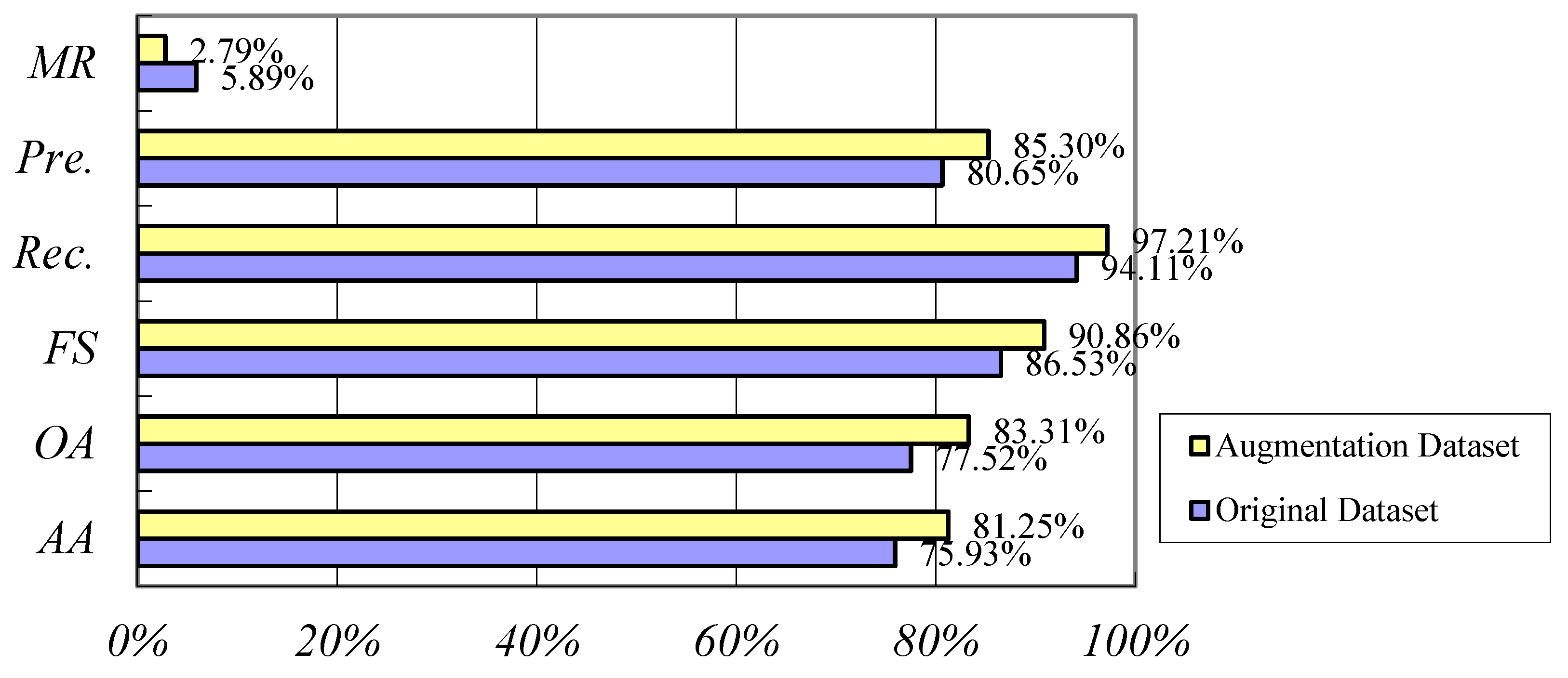
4.3. Experiment Results

The detection performance for each type of component is shown in

Table 4. Detection performance for different objects in test set.

	TP	FP	FN	Pre.	Rec.	MR	FS
Grid	2967	467	25	86.41%	99.16%	0.84%	92.35%
Column	833	158	17	84.03%	98.04%	1.96%	90.50%
Beam	517	108	50	82.67%	91.18%	8.82%	86.71%
Beam_v	500	100	42	83.33%	92.31%	7.69%	87.59%
Beam_s	125	17	8	88.24%	93.75%	6.25%	90.91%

Note: Grid, Column, Beam, Beam_v and Beam_s in the table denote grid references, columns, horizontal beams, vertical beams and sloped beams, respectively.

. It can be seen that grid references have the best results with Pre. of 86.41%, Rec. of 99.16% and FS of 92.35%. The reason for this situation is that grid references appear most frequently in both CLPIs and FPIs, and their features are more distinctive than other components. On the other hand, horizontal beams are identified with the lowest Pre. of 82.67%, Rec. of 91.18% and FS of 86.71% as well as the highest MR of 8.82%. It demonstrates that beams, especially referring to those placing horizontally on 2D drawings, cannot be accurately recognized by YOLO in some cases. For example, when the aspect ratio of the beam is too large, the horizontal beam is often neglected to detect. When the aspect ratio is small, this type of beam is easily identified as a vertical beam. A horizontal beam tends to be identified as a column if its aspect ratio is close to 1. In addition, it also can be observed from Table 4 that the Pre. of all components is lower than their Rec. According to the definitions of precision and recall (Section 4.2.3), this result can be attributed to the fact that FP is always greater than FN for each type of component. In other words, other components are frequently misidentified as this kind of component during the process of object detection.

In addition to the aforementioned metrics, OA, AA and speed of component detection by YOLO are also evaluated in this experiment. It can be seen from

Table 5. TD, TA, OA, AA, and speed for different objects in test set.

	TD	TA	OA	AA	Speed
Grid	3459	3125	85.78%	82.67%	-
Column	1008	925	82.64%	80.18%	-
Beam	675	583	76.54%	77.14%	-
Beam_v	642	583	77.92%	78.57%	-
Beam_s	150	142	83.33%	85.00%	-
Average	2338	2113	83.31%	81.25%	0.71 s

that grid references and vertical beams have the highest OA and AA, while horizontal beams perform the worst in these two metrics. Moreover, the total averages of OA and AA for the whole image rather than for one type of component are calculated as comprehensive performance indexes to measure the detection results of the image when using YOLO. Since large differences between the total amount of each class exist (for instance, the number of grid references is about 20 times than that of sloped beams), weighted average method instead of arithmetic average method is applied in this study to obtain these two image-level accuracies. The equation for calculating these two metrics is (x₁N₁ + x₂N₂ + … + x_kN_k)/k, where x_i (i = 1, 2… k) represents the OA or AA for each class of component, and N_j (i = 1, 2… k) denotes the actual total number component of each class. Referring to Table 5, the total average of OA reaches 83.31%, with 81.25% of the components in image being correctly recognized. Also, the average computing time for an image is 0.71 s. These results demonstrate that the proposed YOLO-based method has the ability to detect multiple structural components from structural 2D drawings with comparatively high accuracy and a short detection time.

5. Discussion

During the process of component detection with YOLO, many factors, such as the size of dataset and the number of components in images, may have a significant impact on final detection results. Therefore, several accuracy-influencing factors are discussed in this section. Moreover, the errors generated in this research are also analyzed.

5.1. Accuracy-Influencing Factors Analysis

5.1.1. The Size of Dataset

Generally, in the field of object detection, with the increase of the training dataset, the effect of detection will be improved. This is because the neural network will constantly adjust the weights in the hidden layer during the training process. The larger the dataset is, the smaller the error of the result will be as well as the risk of overfitting, and the closer the detection result will be to the truth. In this paper, the detection effect of structural components using YOLO is tested under the original dataset and the augmented dataset. Since each image in each different dataset contains a different number of structural components, for a better understanding, the weighted averages of several metrics (like Pre., Rec., MR, FS, OA and AA) are calculated to measure the detection performance of YOLO in a different dataset.

According to Figure 6, it is obviously observed that the YOLO-based method trained by the augmented dataset receives much better results with Pre. of 85.30%, Rec. of 97.21% and FS of 90.86%, and OA and AA are improved by 5.79% and 5.32%, respectively. Meanwhile, MR decreases from 5.89% to 2.79%. Therefore, the thorough improvements using the augmented dataset rather than the original dataset demonstrate that the size of the dataset does have a marked impact on the performance of object detection. When using more data for training YOLO, the better the result of structural object detection will be obtained.

5.1.2. The Number of Components in the Image

Another factor that affects the accuracy of the structural component detection is the number of components to be detected in the image of 2D drawings. With the fixed resolution of the input image, if more components are contained in an image, each component will occupy a smaller pixel size and have less features. Consequently, the probability of missing or false detection will increase when classifying the structural components based on YOLO. To verify the relationship expounded above, in this paper, 300 images of structural drawings used for testing are classified into CLPIs and FPIs, and the total number of components in each image is counted. After that, the average of OA and AA for each image are calculated based on FP, TP, FN, and total number of components. The relationships between the number of structural objects and the detection accuracy in CLPI and FPI are shown in Figure 7.

In Figure 7a, the total numbers of structural components of each CLPI in the test set range from 10 to 25. Meanwhile, the average OA and AA of CLPI decrease with the number of components increasing. The maximum average OA of 95.42% and AA of 93.67% are obtained in CLPI with 10 components, while the minimum average OA of 80.07% and AA of 77.81% are acquired in the image with 25 components. The same trend also happens with FPI, as shown in Figure 7b. Moreover, it is distinctly noticed that the value of average OA (95.01%) is nearly equal to the value of average AA (94.06%) when the number of structural objects in FPI is small. As the number of components increases, the declining trend of AA is bigger than that of OA. The main reason for this inconsistency, based on the definitions of OA and AA explained in Section 4.2.3, is that more missing errors are produced during the detection process rather than classification errors. Therefore, based on the aforementioned analysis, it can be concluded that the number of structural components does have a significant impact on the accuracy of structural component detection.

5.1.3. Other Factors

Other factors, such as the hyperparameter of YOLO and the size of image resolution, also have effects on the detection result of structural components. Hyperparameter refers to the parameter that is preset based on the experience before training rather than obtained through training. The selection of the hyperparameter has a significant influence on the detection results. For instance, the batch size, which is one of the most common hyperparameters, represents the number of samples sent into the model of the neural network in each training. Generally, the smaller batch size is prone to longer training time and non-convergence of the model, while the larger batch size makes the model converge faster, but easily results in the out-of-memory error or program crash. Therefore, choosing the appropriate batch size within a reasonable range can achieve the best balance between time and accuracy when training the YOLO model. Moreover, raising the size of the input image may also affect the accuracy of the structural component detection based on YOLO. This is because when the size of image resolution increases, the number of pixels occupied by a single component will also increase. In consequence, the image features of each component will be richer than before. A disadvantage of raising the image size is that it greatly increases the computing workload as well as the time for training.

5.2. Error Analysis

In order to further analyze the recognition results of the structural components, the errors resulted from the proposed YOLO-based method are divided into five categories based on their types: localization error, background error, similarity error, classification error, and missing error [55]. Localization error indicates that the classification result is correct but the location of the bounding box is biased and not rightly enclosing the structural component. On the contrary, classification error happens when the bounding box locates at the right place while the target object is detected in other categories. Background error means that a bounding box appears in background areas without any component. Similarity error occurs when two or more bounding box exist for one target object, and missing error refers to the situation where the structural components in the image of 2D drawings are not detected. The causes of different types of errors vary from each other, but most of them are closely linked to the selected neural network. For instance, in YOLO used in this paper, each grid predicts two bounding boxes to detect the structural components whose coordinates of central position fall within the grid area. This may lead to missing error if the centers of multiple components fall in the same grid.

Similar to the method mentioned in Section 4.3, the weighted average method was adopted to calculate the average proportion of all kinds of errors across five classes. As shown in

Table 6. Proportion of different types of errors across five classes of components.

	Correct	Localization	Background	Similarity	Classification	Missing
Average	69.54%	10.09%	8.03%	5.65%	2.26%	4.43%

, when using YOLO for structural component detection, 69.54% of the images are correctly recognized, while 30.46% of the detections have errors. It is also obviously noticed that localization error is the largest of all errors and is about five times the total amount of classification error, which indicates that YOLO has problems with locating the identified components correctly. In addition, 8.03% of detections have background error, and 5.65% and 4.43% of detections have the problems of multi-detection and omission of bounding boxes, respectively.

6. Conclusions

In recent years, BIM has been continuously regarded as a core tool to operate and manage the as-built and as-is buildings. However, the lack of BIM models in existing buildings limits BIM applications in O&M phase. Building 3D models based on 2D engineering drawings is regarded as a feasible way to reconstruct BIM models. As the first step of this kind of method, the accuracy of component detection from 2D drawings and the quality of extraction of corresponding geometric information have a significant impact on the final results of reconstruction. Therefore, in this paper, a novel component detection method based on YOLO was proposed to quickly and accurately identify structural components in scanned structural drawings. The experimental results show that Pre. and Rec. for all five classes are above 80% as well as the average of OA and AA for the entire image. Moreover, the average time for identifying an image is only 0.71 s. All these results strongly prove the feasibility and potential of the proposed YOLO-based method for recognizing components from 2D structural drawings.

The main contribution of this study is that it opens up a new way to detect structural components for reconstructing a BIM model of existing buildings from paper-based 2D drawings. Also, it is of important referential value for the application of the deep learning-based component detection method in other professions like architecture and mechanical systems. The second contribution is that it clearly certifies the advantages of the proposed method over traditional component recognition methods. Compared with the existing approaches mentioned in Section 2.1, YOLO-based method not only guarantees the accuracy of components detection, but also has more advantages in detection speed and cost. What is more, the method proposed in this paper has the trait of universality due to its powerful learning ability, which means it can detect components in scanned 2D drawings generated in different countries and design conventions if the training data is sufficient. The final contribution of this study is that several optimal experiment settings have been found for better performance of the proposed YOLO-based method, though there is still room for improvement. It offers some references for the following researchers to improve the work mentioned in this paper.

Additionally, the method proposed in this study can be further improved. The future research work is concluded as follows:

• The experiment of component detection in this paper is focused on limited structural components (e.g., beam and column). To further improve the proposed method, more structural elements (such as floor, shear wall and pile) need to be tested in future research.
• More advanced YOLOv2 with batch normalization, high resolution classifier, anchor box, and multi-scale training will be tried. In addition, more sensitivity analysis will be conducted to study the influence of various accuracy-influencing factors on the final recognition results.
• Last but not least, as the first step to reconstruct BIM models for existing buildings, this study only solves the problem of extracting geometric information of structural components. How to extract topological and semantic information and match with the corresponding components will be the key research direction in the future.

References

1. Volk, J.; Stengel, J.; Schultmann, F. Building information modeling (BIM) for existing buildings—Literature review and future needs. Autom. Constr. 2014, 38, 109–127. [Google Scholar] [CrossRef] [Green Version]
2. Becerik-Gerber, B.; Jazizadeh, F.; Li, N.; Calis, G. Application areas and data requirements for BIM-enabled facilities management. J. Constr. Eng. Manag. 2012, 138, 431–442. [Google Scholar] [CrossRef]
3. Akcamete, A.; Akinci, B.; Garrett, J.H. Potential utilization of building information models for planning maintenance activities. In Proceedings of the 13th International Conference on Computing in Civil and Building Engineering, Nottingham, UK, 30 June–2 July 2010; pp. 8–16. [Google Scholar]
4. Hu, Z.Z.; Peng, Y.; Tian, P.L. A review for researches and applications of BIM-based operation and maintenance management. J. Graph. 2015, 36, 802–810. [Google Scholar]
5. Gimenez, L.; Hippolyte, J.; Robert, S.; Suard, F.; Zreik, K. Review: Reconstruction of 3d building in-formation models from 2d scanned plans. J. Build. Eng. 2015, 2, 24–35. [Google Scholar] [CrossRef]
6. Li, J.; Huang, W.; Shao, L.; Allinson, N. Building recognition in urban environments: A survey of state-of-the-art and future challenges. Inf. Sci. 2014, 277, 406–420. [Google Scholar] [CrossRef]
7. Tang, P.B.; Huber, D.; Akinci, B.; Lipman, R.; Lytle, A. Automatic reconstruction of as-built building information models from laser-scanned point clouds: A review of related techniques. Autom. Constr. 2010, 19, 829–843. [Google Scholar] [CrossRef]
8. Cho, C.Y.; Liu, X. An automated reconstruction approach of mechanical systems in building infor-mation modeling (BIM) using 2d drawings. In Proceedings of the ASCE International Workshop on Computing in Civil Engineering 2017, Seattle, WA, USA, 25–27 June 2017; pp. 236–244. [Google Scholar]
9. Gimenez, L.; Robert, S.; Suard, F.; Zreik, K. Automatic reconstruction of 3d building models from scanned 2D floor plans. Autom. Constr. 2016, 63, 48–56. [Google Scholar] [CrossRef]
10. Huang, H.C.; Lo, S.M.; Zhi, G.S.; Yuen, R.K.K. Graph theory-based approach for automatic recognition of cad data. Eng. Appl. Artif. Intell. 2008, 21, 1073–1079. [Google Scholar] [CrossRef]
11. Yin, X.; Wonka, P.; Razdan, A. Generating 3d building models from architectural drawings: A survey. IEEE Comput. Graph. Appl. 2008, 29, 20–30. [Google Scholar] [CrossRef]
12. Klein, L.; Li, N.; Becerik-Gerber, B. Imaged-based verification of as-built documentation of operational buildings. Autom. Constr. 2012, 21, 161–171. [Google Scholar] [CrossRef]
13. Dominguez, B.; Garcia, A.L.; Feito, F.R. Semiautomatic detection of floor topology from CAD architectural drawings. Comput. Aided Des. 2012, 44, 367–378. [Google Scholar] [CrossRef]
14. Lu, Q.C.; Lee, S.; Chen, L. Image-driven fuzzy-based system to construct as-is IFC BIM objects. Autom. Constr. 2018, 92, 68–87. [Google Scholar] [CrossRef]
15. Hough, P.V.C. Method and Means for Recognizing Complex Patterns. U.S. Patent 3,069,654, 18 December 1962. [Google Scholar]
16. Lowe, D.G. Object recognition from local scale-Invariant features. In Proceedings of the Seventh I-EEE International Conference on Computer Vision, Kerkyra, Greece, 20–27 September 1999; pp. 1150–1157. [Google Scholar]
17. Matas, J.; Chum, O.; Urban, M.; Pajdla, T. Robust wide baseline stereo from maximally stable extremal regions. Image Vis. Comput. 2004, 22, 761–767. [Google Scholar] [CrossRef]
18. Bay, H.; Ess, A.; Tuytelaars, T.; Gool, L.V. Speeded-up robust features (SURF). Comput. Vis. Image Underst. 2008, 110, 346–359. [Google Scholar] [CrossRef]
19. Mukhopadhyay, P.; Chaudhuri, B.B. A survey of Hough Transform. Pattern Recognit. 2015, 48, 993–1010. [Google Scholar] [CrossRef]
20. Ballard, D.H. Generalizing the Hough Transform to detect arbitrary shapes. Pattern Recognit. 1981, 13, 111–122. [Google Scholar] [CrossRef]
21. Galambos, C.; Kittler, J.; Matas, J. Gradient based progressive probabilistic Hough Transform. IEE Proc. Vis. Image Signal Process. 2001, 148, 158. [Google Scholar] [CrossRef] [Green Version]
22. Xu, L.; Oja, E.; Kultanen, P. A new curve detection method: Randomized Hough transform (RHT). Pattern Recognit. Lett. 1990, 11, 331–338. [Google Scholar] [CrossRef]
23. Kiryati, N.; Lindenbaum, M.; Bruckstein, A.M. Digital or analog hough transform? Pattern Recognit. Lett. 1991, 12, 291–297. [Google Scholar] [CrossRef] [Green Version]
24. Izadinia, H.; Sadeghi, F.; Ebadzadeh, M.M. Fuzzy generalized hough transform invariant to rotation and scale in noisy environment. In Proceedings of the IEEE International Conference on Fuzzy Systems, Jeju Island, Korea, 20–24 August 2009; pp. 153–158. [Google Scholar]
25. Dosch, P.; Tombre, K.; Ah-Soon, C.; Masini, G. A complete system for the analysis of architectural drawings. Int. J. Doc. Anal. Recognit. 2000, 3, 102–116. [Google Scholar] [CrossRef]
26. Mace, S.; Locteau, H.; Valveny, E.; Tabbone, S. A system to detect rooms in architectural floor plan images. In Proceedings of the Ninth IAPR International Workshop on Document Analysis Systems, Boston, MA, USA, 9–11 June 2010; pp. 167–174. [Google Scholar]
27. Ahmed, S.; Liwicki, M.; Weber, M.; Dengel, A. Improved automatic analysis of architectural floor plans. In Proceedings of the 2011 International Conference on Document Analysis and Recognition, Beijing, China, 18–21 September 2011; pp. 864–869. [Google Scholar]
28. Riedinger, C.; Jordan, M.; Tabia, H. 3D models over the centuries: From old floor plans to 3D representation. In Proceedings of the 2014 International Conference on 3D Imaging, Liege, Belgium, 9–10 December 2014; pp. 1–8. [Google Scholar]
29. Lu, T.; Yang, H.F.; Yang, R.Y.; Cai, S.J. Automatic analysis and integration of architectural drawings. Int. J. Doc. Anal. Recognit. 2007, 9, 31–47. [Google Scholar] [CrossRef]
30. Lu, Q.C.; Lee, S. A semi-automatic approach to detect structural components from CAD drawings for constructing as-Is BIM objects. In Proceedings of the ASCE International Workshop on Computing in Civil Engineering 2017, Seattle, WA, USA, 25–27 June 2017; pp. 84–91. [Google Scholar]
31. Fang, Q.; Li, H.; Luo, X.C.; Ding, L.Y.; Luo, H.B.; Rose, T.M.; An, W.P. Detecting non-hardhat-use by a deep learning method from far-field surveillance videos. Autom. Constr. 2018, 85, 1–9. [Google Scholar] [CrossRef]
32. Fang, Q.; Li, H.; Luo, X.C.; Ding, L.Y.; Luo, H.B.; Li, C. Computer vision aided inspection on falling prevention measures for steeplejacks in an aerial environment. Autom. Constr. 2018, 93, 148–164. [Google Scholar] [CrossRef]
33. Zhang, A.; Wang, K.C.P.; Li, B.X.; Yang, E.; Dai, X.X.; Yi, P.; Fei, Y.; Liu, Y.; Li, J.Q.; Chen, C. Automated pixel-level pavement crack detection on 3d asphalt surfaces using a deep-learning network. Comput. Aided Civ. Infrastruct. Eng. 2017, 32, 805–819. [Google Scholar] [CrossRef]
34. Wu, D.; Pigou, L.; Kindermans, P.J.; Le, N.D.H.; Shao, L.; Dambre, J.; Odobez, J.M. Deep dynamic neural networks for multimodal gesture segmentation and recognition. IEEE Trans. Pattern Anal. Mach. Intell. 2016, 38, 1583–1597. [Google Scholar] [CrossRef] [PubMed] [Green Version]
35. Gangwar, A.; Joshi, A. DeepIrisNet: Deep iris representation with applications in iris recognition and cross-sensor iris recognition. In Proceedings of the IEEE International Conference on Image Processing, Phoenix, AZ, USA, 25–28 September 2016. [Google Scholar]
36. Hu, C.; Bai, X.; Qi, L.; Chen, P.; Xue, G.; Mei, L. Vehicle color recognition with spatial pyramid deep learning. IEEE Trans. Intell. Transp. Syst. 2015, 16, 2925–2934. [Google Scholar] [CrossRef]
37. Saxena, S.; Verbeek, J. Heterogeneous face recognition with CNNs. In Proceedings of the 14th European Conference on Computer Vision, Amsterdam, The Netherlands, 11–14 October 2016; pp. 483–491. [Google Scholar]
38. Kong, Y.; Ding, Z.; Li, J.; Fu, Y. Deeply learned view-invariant features for cross-view action recognition. IEEE Trans. Image Process. 2017, 26, 3028–3037. [Google Scholar] [CrossRef] [PubMed]
39. Girshick, R.; Donahue, J.; Darrell, T.; Malik, J. Rich feature hierarchies for accurate object detection and semantic segmentation. In Proceedings of the 2014 IEEE Conference on Computer Vision and Pattern Recognition, Columbus, OH, USA, 23–28 June 2014; pp. 580–587. [Google Scholar]
40. Uijlings, J.R.R.; Sande, K.E.A.; Gevers, T. Selective search for object recognition. Int. J. Comput. Vis. 2013, 104, 154–171. [Google Scholar] [CrossRef] [Green Version]
41. Girshick, R. Fast R-CNN. In Proceedings of the 2015 IEEE International Conference on Computer Vision, Santiago, Chile, 7–13 December 2015; pp. 1440–1448. [Google Scholar]
42. He, K.M.; Zhang, X.Y.; Ren, S.Q.; Sun, J. Spatial pyramid pooling in deep convolutional networks for visual recognition. In Proceedings of the 13th European Conference on Computer Vision, Zurich, Switzerland, 6–12 September 2014; pp. 1904–1916. [Google Scholar]
43. Ren, S.Q.; He, K.M.; Girshick, R.; Sun, J. Faster R-CNN: Towards real-time object detection with re-gion proposal networks. IEEE Trans. Pattern Anal. Mach. Intell. 2017, 39, 1137–1149. [Google Scholar] [CrossRef] [Green Version]
44. He, K.M.; Gkioxari, G.; Dollár, P.; Girshick, R. Mask R-CNN. In Proceedings of the 2017 IEEE International Conference on Computer Vision, Venice, Italy, 22–29 October 2017. [Google Scholar]
45. Redmon, J.; Divvala, S.; Girshick, R.; Farhadi, A. You only look once: Unified, real-time object detection. In Proceedings of the 2016 IEEE Conference on Computer Vision and Pattern Recognition, Las Vegas, NV, USA, 27–30 June 2016; pp. 779–788. [Google Scholar]
46. Liu, W.; Anguelov, D.; Erhan, D.; Szegedy, C.; Reed, S.; Fu, C.Y.; Berg, A.C. SSD: Single shot multibox detector. In Proceedings of the 14th European Conference on Computer Vision, Amsterdam, The Netherlands, 11–14 October 2016; pp. 21–37. [Google Scholar]
47. Redmon, J.; Farhadi, A. YOLO9000: Better, faster, stronger. In Proceedings of the IEEE Conference on Computer Vision and Pattern Recognition, Honolulu, HI, USA, 21–26 July 2017. [Google Scholar]
48. Russakovsky, O.; Deng, J.; Su, H.; Krause, J.; Satheesh, S.; Ma, S.; Huang, Z.; Karpathy, A.; Khosla, A.; Bernstein, M.; et al. ImageNet large scale visual recognition challenge. Int. J. Comput. Vis. 2014, 115, 211–252. [Google Scholar] [CrossRef] [Green Version]
49. Lin, T.Y.; Maire, M.; Belongie, S.; Hays, J.; Perona, P.; Ramanan, D.; Dollár, P.; Zitnick, C.L. Microsoft COCO: Common objects in context. In Proceedings of the 13th European Conference on Computer Vision, Zurich, Switzerland, 6–12 September 2014; pp. 740–755. [Google Scholar]
50. Yang, H.; Zhou, X. Deep learning-based ID card recognition method. China Comput. Commun. 2016, 21, 83–85. [Google Scholar]
51. Gonzalez, R.C.; Woods, R.E. Digital Image Processing, 3rd ed.; Pearson Prentice Hall: Upper Saddle River, NJ, USA, 2008. [Google Scholar]
52. Neubeck, A.; Gool, L.V. Efficient non-maximum suppression. In Proceedings of the 18th International Conference on Pattern Recognition, Hong Kong, China, 20–24 August 2006; pp. 850–855. [Google Scholar]
53. LabelImg. Available online: https://github.com/tzutalin/labelImg (accessed on 15 October 2019).
54. Opencv. Available online: https://opencv.org (accessed on 20 December 2019).
55. Hoiem, D.; Chodpathumwan, Y.; Dai, Q. Diagnosing error in object detectors. In Proceedings of the 12th European Conference on Computer Vision, Florence, Italy, 7–13 October 2012. [Google Scholar]
Figure 1. Overall process of YOLO-based component detection method.
Applsci 10 02066 g001
Figure 2. Image preprocessing results in different phases.
Applsci 10 02066 g002
Figure 3. The prediction information contained in each grid cell.
Applsci 10 02066 g003
Figure 4. Example of output for component detection result.
Applsci 10 02066 g004
Figure 5. Labeling components in the image of structural drawings.
Applsci 10 02066 g005
Figure 6. Comparison of the performance in different sizes of datasets via YOLO.
Applsci 10 02066 g006
Figure 7. The relation between the number of structural components and the detection accuracy: (a) In the column layout plan image; (b) In the framing plan image.
Applsci 10 02066 g007