Article

Asymptotic Performance Analysis of the MUSIC Algorithm for Direction-of-Arrival Estimation

1
Smart Mobility Research Section, Electronics and Telecommunications Research Institute Daegu-Gyeongbuk Research Center, Daegu 42994, Korea
2
MFG HQ Qutomation TFT, Amkor Technology Korea, Inc., Incheon 21991, Korea
3
Department of Information and Communication Engineering, Sejong University, Seoul 05006, Korea
*
Author to whom correspondence should be addressed.
Appl. Sci. 2020, 10(6), 2063; https://doi.org/10.3390/app10062063
Submission received: 29 January 2020 / Revised: 5 March 2020 / Accepted: 12 March 2020 / Published: 18 March 2020
(This article belongs to the Special Issue Recent Advances in Electronic Warfare Networks and Scenarios)

Abstract

:
We consider the performance analysis of the multiple signal classification (MUSIC) algorithm for multiple incident signals when the uniform linear array (ULA) is adopted for estimation of the azimuth of each incident signal. We derive closed-form expression of the estimation error for each incident signal. After some approximations, we derive closed-form expression of the mean square error (MSE) for each incident signal. In the MUSIC algorithm, the eigenvectors of covariance matrix are used for calculation of the MUSIC spectrum. Our derivation is based on how the eigenvectors of the sample covariance matrix are related to those of the true covariance matrix. The main contribution of this paper is the reduction in computational complexity for the performance analysis of the MUSIC algorithm in comparison with the traditional Monte–Carlo simulation-based performance analysis. The validity of the derived expressions is shown using the numerical results. Future work includes an extension to performance analysis of the MUSIC algorithm for simultaneous estimation of the azimuth and the elevation.

1. Introduction

The multiple signal classification (MUSIC) algorithm [1] has been one of the most widely used direction-of-arrival (DOA) algorithms [2,3]. It exploits the orthogonality between the noise eigenvectors of the covariance matrix and the array vectors associated with the true angles of the incident signals. Since the noise subspace is orthogonal to the signal subspace, the array vectors corresponding to the true incident angles should belong to the signal subspace of the covariance matrix.
In practice, the covariance matrix itself, which is defined from the ensemble average, is not usually available, and the sample covariance matrix is obtained from time average. In the assumption of the ergodicity, the covariance matrix can be replaced with the sample covariance matrix when the number of snapshots is very large. When the number of snapshots is finite, the time-average-based sample covariance is not equal to the ensemble-average-based true covariance matrix.
Since the true covariance matrix is not available, we use the eigenvectors of the sample covariance matrix, not the eigenvectors of the true covariance matrix. When the number of the snapshots is finite, the eigenvectors of the sample covariance matrix are not identical to those of the covariance matrix due to the difference between the true covariance matrix and the sample covariance matrix.
Although the array vectors corresponding to the true incident angles belong to the signal subspace of the true covariance matrix, the array vector corresponding to the true incident angles do not belong to the signal subspace of the sample covariance matrix. Note that, in the MUSIC algorithm, angles spanning the signal subspace of the sample covariance matrix, not the true covariance matrix, are used as estimates of incident signals since true covariance matrix is not available. The mathematical and statistical theories used for derivation of the results are as follows:
Statistical description of perturbations
How various perturbations can be statistically described in terms of probability density function, moments to get a closed-form expression of the MSE of the estimate.
Taylor series
How Taylor series can be adopted to obtain explicit expression of the MSE of the estimate
Eigenvector perturbation and eigenvalue perturbation
How the eigenvectors and the eigenvalues of a matrix are perturbed due to the perturbations in the entries of the matrix.
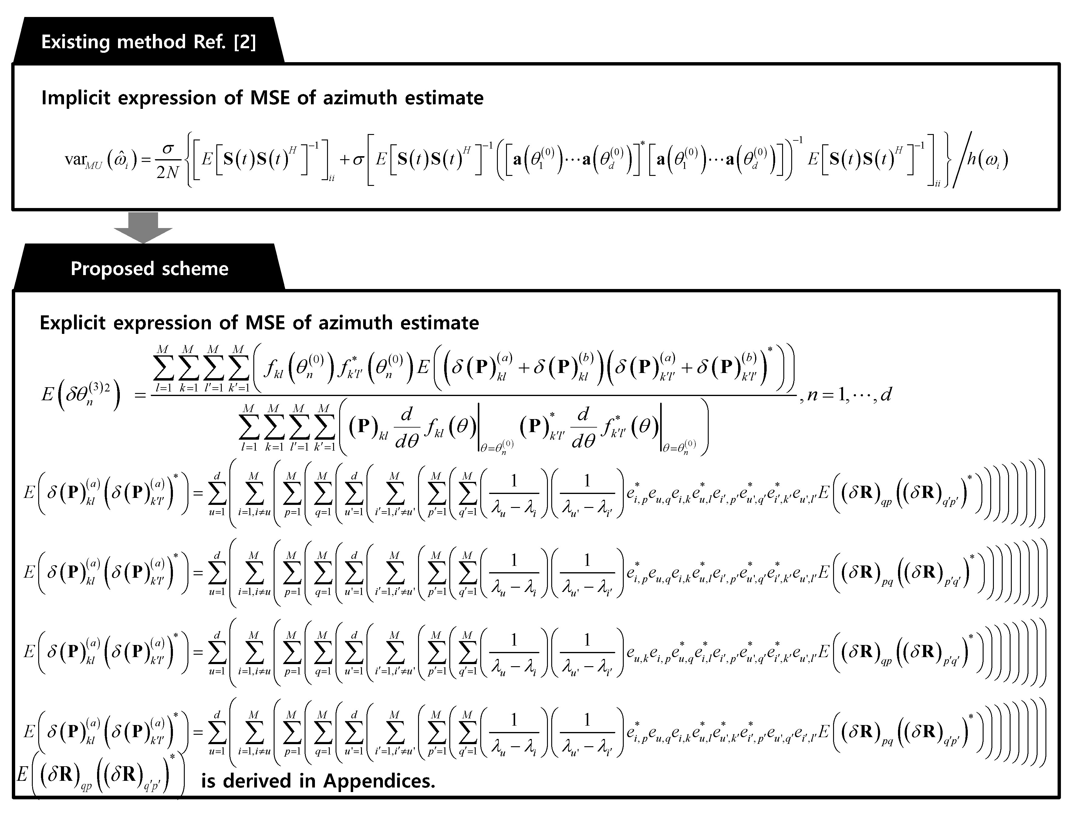
In [2], the authors carried out a performance analysis of the MUSIC algorithm and derived an implicit expression of the estimate. On the other hand, in this paper, explicit expressions of the estimate itself and the MSE of the estimate have been derived. In Figure 1, the performance analysis proposed in this paper is summarized. Figure 2 clearly indicates how the proposed scheme in this paper is different from the existing performance analysis of the MUSIC algorithm in [2]. In this paper, we obtain the explicit expressions of θ n ( 1 ) , θ n ( 2 ) and θ n ( 3 ) . The estimate with superscript (1) denotes the estimate of the original MUSIC algorithm. Note that no approximation is used in getting the estimate with superscript (1). The estimate with superscript (2) denotes the estimate based on the first approximation, and that with superscript (3) represents the estimate based on the first approximation and the second approximation.
The difference between θ n ( 1 ) and θ n ( 2 ) quantifies the error due to the first approximation since the first approximation is applied in getting θ n ( 2 ) . Note that no approximation is applied in getting θ n ( 1 ) . Similarly, the difference between θ n ( 2 ) and θ n ( 3 ) quantifies the error due to the second approximation since the first approximation and the second approximations are applied in getting θ n ( 3 ) . Based on this intuition, by comparing θ n ( 1 ) , θ n ( 2 ) and θ n ( 3 ) , we can easily determine which approximation results in the dominant approximation error. This inspection cannot be obtained from the scheme presented in the previous study [2].
As far as the authors know, no previous study on the performance analysis of the MUSIC algorithm presented explicit expressions of each estimate in successive approximations [4,5,6,7,8,9,10]. Depending on how many approximations out of all the approximations are applied, the estimates for all the intermediate stages are rigorously derived in this paper.
In this paper, we consider the case in which multiple signals are incident on the uniform linear array (ULA). To quantify the difference between the signal subspace of the true covariance matrix and that of the sample covariance matrix, the Taylor series expansion is adopted to get an analytic expression of the MSE.
For getting θ n ( 1 ) , for n = 1 , , d , in the original MUSIC algorithm, the MUSIC spectrum has to be evaluated as the azimuth angle takes discrete search angles. Note that d denotes the number of incident signals. To estimate both azimuth and elevation, the MUSIC spectrum has to evaluated as two variables of azimuth and elevation take discrete search angles, which can be computationally intensive, especially for small increments of the azimuth and the elevation. Note that the estimate is obtained from the search angle which optimizes the MUSIC cost function. Therefore, in the original MUSIC algorithm, the final estimate depends on how the search range and the search step are chosen. Improperly chosen search angles in the MUSIC algorithm implementation result in an inaccurate estimate, which degrades the performance of the original MUSIC algorithm.
In short, there are two problems in getting θ n ( 1 ) : Firstly, it can be computationally intensive for simultaneous estimation of azimuth and elevation. Secondly, the estimate is highly dependent on the selection of the search range and the search step.
It is described how the first problem with θ n ( 1 ) can be overcome by adopting δ θ n ( 2 ) and δ θ n ( 3 ) proposed in this paper. δ θ n ( 2 ) is given by (38), and δ θ n ( 3 ) is given by (39). Since (38) and (39) are closed-form expressions, evaluation of δ θ n ( 2 ) and δ θ n ( 3 ) does not require computationally intensive exhaustive search over search angles. Therefore, getting δ θ n ( 2 ) and δ θ n ( 3 ) is much less computationally intensive than getting θ n ( 1 ) .
The second problem with θ n ( 1 ) can also be circumvented. Since δ θ n ( 2 ) and δ θ n ( 3 ) are analytically given by (38) and (39), they do not depend on the choice of search parameters such as the search step and the search range.
To get δ θ n ( 2 ) analytically from (38), the first approximation has to be applied to the cost function of the original MUSIC algorithm. On the other hand, in getting θ n ( 1 ) , no approximation is applied to the cost function of the original MUSIC algorithm. Therefore, δ θ n ( 2 ) can be regarded as an estimation error associated with the approximated cost function.
Similarly, to get δ θ n ( 3 ) analytically from (39), the first approximation and the second approximation should be applied to the cost function of the original MUSIC algorithm. Although θ n ( 1 ) is obtained from an exhaustive search of the cost function of the original MUSIC algorithm, no approximation is applied to get θ n ( 1 ) . δ θ n ( 3 ) can also be regarded as an estimation error associated with the approximated cost function.
Due to search-free characteristics of evaluating (38) and (39), single evaluation of (38) and (39) once is not computationally intensive at all. On the other hand, many evaluations of (38) and (39) can be computationally intensive, especially for large number of repetitions. Note that (38) and (39) should be evaluated many times to empirically quantify the accuracy of δ θ n ( 2 ) and δ θ n ( 3 ) and that the number of repetitions should be large enough to make the estimated accuracy more reliable.
To obviate this problem, it is shown in this paper that the MSE of δ θ n ( 3 ) can be analytically given by (40). Empirical MSE from many evaluations of (39) can be replaced with analytic MSE given by (40): single evaluation of (40) is much less computationally intensive than many evaluations of (39).
It should also be noted that, unlike δ θ n ( 3 ) , it is impossible to get an analytic expression of the MSE of δ θ n ( 2 ) . Therefore, the MSE of θ n ( 2 ) should be evaluated empirically from many evaluations of (38). Different realization of Gaussian-distributed noise should be used for each evaluation of (38). In summary, the performance of the MUSIC algorithm can be evaluated very efficiently via (40) in comparison with the Monte–Carlo simulation-based performance analysis.
The rest of this paper is structured as follows. In Section 2, we explain how the notation can be used to describe the proposed method. In Section 3, we address the conventional MUSIC algorithm. In Section 4, the explicit expression of the difference between the true covariance matrix and the sample covariance matrix has been derived. In Section 5, we have derived an expression of difference between the signal eigenvector of the true covariance matrix and that of the sample covariance matrix in terms of the difference between the true covariance matrix and the sample covariance matrix. In Section 6, a few closed-form expressions of an estimation error, depending on whether specific approximation is applied or not, are derived. In Section 7, for one of the many closed-form expressions of an estimation error, we have derived an explicit representation of the estimate accuracy in terms of the MSE. In Section 8, we address performance analysis of the MUSIC algorithm for multiple incident signals. The simulation results are shown to validate the closed-form estimation error of the proposed method in comparison with an estimation error of the conventional MUSIC method.
In [11], an explicit closed-form expression of the MSE of the direction-of-arrival (DOA) estimation algorithm based on maximum-likelihood (ML) criterion is presented. On the other hand, in this paper, the performance analysis of the MUSIC DOA estimation algorithm for the uniform linear array is proposed. In [11], the derivation is based on the Taylor series expansion of the sample covariance matrix itself since the cost function of the ML DOA estimation algorithm can be explicitly written in terms of the sample covariance matrix. In this paper, we adopt the Taylor series expansion of the eigenvectors of the sample covariance matrix, not the Taylor series expansion of the sample covariance matrix itself, since the cost function of the MUSIC algorithm can be written in terms of the eigenvectors of the sample covariance matrix, not in terms of the sample covariance matrix.
In [12], the authors have presented the statistical analysis of MUSIC algorithm for general sparse linear arrays in the presence of sensor location uncertainty. Both cases of deterministic sensor location error and stochastic sensor location error have been considered.
In [13], the authors have considered basis mismatch problem in DOA estimation. The authors have indicated why dense sampling grids cannot solve basis mismatch problem completely, and they proposed new scheme which is superior to the previous method for handling basis mismatch problem. The superiority of the proposed scheme has been validated in terms of computational complexity and estimation accuracy.
In [14], the authors have presented a new scheme, called sG-MUSIC, which is superior to the previous G-MUSIC algorithm in the viewpoint of a bias of the estimate. The authors have shown that the scheme is quite effective when the number of snapshots is small.
In [15], the authors have proposed how the dimension of DOA estimation can be reduced when only a few snapshots are available. The scheme can be applied to 2D-DOA estimation as well as 1-D DOA estimation.
In [16], the authors have presented the performance analysis of G-MUSIC algorithm. The authors have shown in what situation G-MUSIC is superior to the original MUSIC algorithm. The authors have also presented asymptotic variances of G-MUSIC.
There has been a great deal of research on the determination of emitter location. Localization algorithm consists of two parts: measuring localization parameters between nodes, and the use of these parameters to estimate location. The localization parameters can be angle-of-arrival (AOA), time-difference-of-arrival (TDOA), frequency-difference-of-arrival (FDOA), and received signal strength (RSS). In this paper, we consider performance analysis of the MUSIC algorithm, which is one of the DOA estimation algorithms. The DOA estimation is the main application of array signal processing. Radar and sonar are also good examples of the application of array signal processing.
The authors have presented performance analysis for use with amplitude comparison monopulse DOA algorithm under measurement uncertainty. The derived results can be used for determining how the performance of the amplitude comparison monopulse algorithm degrades due to an additive measurement noise without computationally intensive Monte–Carlo simulation. The difference between the scheme in [17] and the proposed scheme in this paper is as follows: the scheme in [17] deals with the performance analysis of monopulse algorithm, which is usually used in tracking radar in the sense that an initial estimate of the DOA should be given in advance. This paper deals with the performance analysis of the MUSIC algorithm, where an initial estimate is not required.
In monopulse algorithm, the tracking radar transmits a radar signal and uses a reflected signal from a radar target to update the DOA. On the other hand, in MUSIC algorithm, direction-finding (DF) station does not transmit a signal to estimate the DOA of an emitter: the DF station just receives a signal of an active emitter, and uses a received signal to estimate the DOA of the emitter. Therefore, the monopulse algorithm is an active DOA estimation algorithm, and the MUSIC algorithm is a passive DOA estimation algorithm.
In [18], the authors proposed how to suppress motion-induced phase in frequency modulated continuous wave (FMCW) radar for automotive application. The motion compensation method is not computationally intensive. Conventional beamforming algorithm is used for DOA estimation. Although the authors illustrate that the motion compensated algorithm results in smaller estimation error than the uncompensated algorithm, they do not derive the closed-form expression of the MSE of the azimuth estimate: the authors illustrate that the peak of the DOA spectrum for the motion-compensated conventional beamforming algorithm is closer to true incident angle than the peak of the DOA spectrum for the original conventional beamforming algorithm. On the other hand, in this paper, the closed-form expression of the MSE of the azimuth estimate for the MUSIC DOA algorithm is presented.
If the MUSIC algorithm, not the conventional beamforming algorithm, is employed for DOA estimation of FMCW radar, the approach leading to Equation (40) of this paper can be applied to get the closed-form expression MSEs of the azimuth estimate both for uncompensated MUSIC algorithm and for compensated MUSIC algorithm. Note that, to obtain the closed-form expression of the MSE of the motion-compensated MUSIC algorithm in [18], the derivation leading to (40) in this paper is modified so that the motion-compensation proposed in [18] can be taken into account in the MUSIC DOA estimation.
In [19], the authors proposed how to improve performance of the minimum variance distortionless response (MVDR) beamforming algorithm by exploiting signal self-cancellation phenomenon in DOA estimation of underwater acoustic sources. The proposed algorithm is called self-signal cancellation MVDR (SCC-MVDR).
In Figures 4 and 5 of [19], they illustrated the root mean square errors (RMSEs) of the MVDR, the MUSIC, the root-MUSIC, TLS-ESPRIT, the propagator method and the SCC-MVDR. The RMSEs are obtained from Equation (17) of [19]: the RMSEs are obtained empirically, not analytically, from the Monte Carlo simulation with the number repetitions of 100. That is, 100 repetitions of the MUSIC algorithm should be performed to get the RMSEs for the MUSIC algorithm. On the other hand, the RMSEs for the MUSIC algorithm can be obtained analytically, without time-consuming repetitive execution of the MUSIC algorithm, by taking the square root of the MSE value in (40) of this paper. In Figure 4 of [19], the RMSEs with respect to SNRs for fixed number of snapshots, 100, are given. In Figure 5 of [19], the RMSEs with respect to the number of snapshots for fixed SNR are presented. Note that, in this paper, the number of snapshots and the SNRs are explicitly taken into account in deriving the MSE in (40), implying that the empirical RMSEs for the MUSIC algorithm in Figures 4 and 5 of [19] can be analytically by taking the square root of the MSE value given by (40). Note that analytical approach is much less computationally intensive than Monte–Carlo simulation-based empirical approach.
In [20], a new DOA estimation algorithm for use with direction estimation of sound source. The preprocessing of the scheme is based on the intuition that isolation of a target speaker can be achieved by selecting dominant time-frequency bin of the time-frequency distribution. Furthermore, neural network approach is employed to finally estimate the DOA of sound source. The performance of the proposed DOA estimation algorithm is given by the mean absolute error (MAE), not the MSE. The MAE is empirically estimated from the Monte–Carlo simulation with the number of repetitions of 200. In summary, they proposed a new DOA estimation algorithm, and the performance of the proposed algorithm is given by the empirically obtained MAE. If the MUSIC algorithm is used for the DOA estimation in the sound source experiment described in [20], the expression in Equation (40) of this paper can be employed to yield the performance of the MUSIC algorithm in terms of the MSE analytically, not empirically.
In [21], the authors are concerned with how to enhance target sound sound when multiple sound sources are present. Preprocessing for the proposed enhancement scheme is to estimate the DOA of the target sound source. That is, the DOA of the sound source should be available for implementation of the proposed target enhancement scheme. In experiment 3 using simulated data and in experiment 5 using recorded data in an anechoic chamber, the authors show how performance of the source enhancement depends on the DOA mismatch, which is the difference between the true DOA and the estimated DOA. If the MUSIC algorithm is employed for preprocessing DOA estimation, the expression in (38) and (39) can be used for calculation of the DOA mismatch.
In the presence of sensor measurement noise, DOA estimate is a random variable. Therefore, it is better to use the MSE of the DOA than to use the DOA mismatch as a measure of DOA estimation accuracy. In that case, the expression in (40) is used to quantify how accurate the DOA estimate for use with the sound source enhancement in [21] is.
In [22], a survey on RSS and AOA-based localization scheme is presented. For the localization scheme to be successful, accurate estimation of RSS and AOA is very important. Performance of localization algorithm is dependent on the estimation accuracy of the RSS and AOA. The scheme presented in this paper can be used for determining the accuracy of the estimates in the MUSIC DOA algorithm, which is one of the most popular DOA algorithms.
In [23], to improve ultrasonic image, Rician beamforming is applied. Sparse sampling in spatial domain is adopted. Basically, beamforming algorithm can be considered as spatial filtering. Beamforming and DOA estimation including the MUSIC algorithm are parts of array signal processing research. Rician beamforming-based array design can be formulated as a convex optimization problem. In this paper, the estimate is obtained from the property that the partial derivative of MUSIC cost function with respect to the azimuth angle at the estimate should be zero: therefore, the estimate of the convex optimization problem can be obtained from the observation that the partial derivative of the cost function with respect to each variable should be zero at an optimal point. Given the estimation error, the MSE can be obtained by exploiting the statistical description of noise or interference.
In [24], a novel beamforming scheme is proposed to improve the previously used beamforming algorithm. Since beamforming technique is a spatial filtering, it can be employed in interference suppression. More specifically, TDMA-beamforming is proposed, and it is shown that the proposed scheme improves the signal to interference plus noise ratio (SINR) by approximately 18 dB.
In [25], a hybrid beamforming employing variable phase shifters (VPSs) and constant phase shifters is proposed. To optimally combine VPSs and CPSs, greedy algorithm is adopted to get a near-optimal solution, since getting exact solution is intractable.
In [26], for improvement of audio enhancement, a new improved distributed minimum variance distortionless response (MVDR) beamforming algorithm is proposed. The algorithm can be applied to wireless acoustic sensor networks. The proposed scheme outperforms two classical methods in the view point of the segmental signal to noise ratio, mean square error, and perceptual evaluation of speech quality.
In Table 1, algorithms, applications, main ideas and contributions of the recently published works are tabulated. In Table 2, it is tabulated how the schemes presented in [17,18,19,20,21,22,23,24,25,26] are validated. In Table 2, it is also described how the explicit expressions of the azimuth estimate and the MSE of the azimuth estimation error derived in this paper can be applied to the problems in [17,18,19,20,21,22,23,24,25,26].

2. Notation

LThe number of snapshots
MThe number of antennas
nThe index of incident signal ( n = 1 , , d )
· T Transpose of a matrix
· H Hermitian of a matrix
· 1 Inverse matrix
E · Statistical expectation
θ n 0 The n-th true azimuth of d incident signals ( n = 1 , , d )
θ ^ n 1 The n-th azimuth estimate in (47)
δ θ n 1 The difference between θ ^ n 1 and θ n 0
θ ^ n 2 The n-th azimuth estimate in (38)
δ θ n 2 The difference between θ ^ n 2 and θ n 0
θ ^ n 3 The n-th azimuth estimate in (39)
δ θ n 3 The difference between θ ^ n 3 and θ n 0
n t i zero-mean Gaussian random vector representing the noise on the antenna
Λ The wavelength of a incident signal
k The unit vector indicating the DOA of the incident signal
z m The coordinate of the m-th antenna
Δ The distance between the adjacent antenna elements
rRadius of antenna array
R The true covariance matrix
R ^ The sample covariance matrix
δ R The difference between the sample covariance and the true covariance matrix
E S The signal eigenvector matrix of R matrix whose columns are the signal eigenvectors of R
E ^ S The signal eigenvector matrix of R ^ matrix whose columns are the signal eigenvectors of R
δ E ^ S The difference between E ^ S and E S
P The projection matrix onto the column space of E S
P ^ The projection matrix onto the column space of E ^ S
δ P The difference between P ^ and P
F θ MUSIC spectrum as a function of azimuth associated with covariance matrix R
F ^ θ MUSIC spectrum as a function of azimuth associated with covariance matrix R ^
F g θ Approximate MUSIC spectrum due to the g-th order approximation of the signal eigenvectors, Approximation of F θ
F g , h θ The h-th Taylor expansion-based approximation of F g ·

3. MUSIC Algorithm

Let θ 1 0 , , θ d 0 represent the true incident angles of d incident signals. The noisy array output vector is written as
x t i = x 1 t i x 2 t i x M t i = x 1 t i + n 1 t i x 2 t i + n 2 t i x M t i + n M t i = exp j ψ 1 θ 1 0 exp j ψ 1 θ d 0 exp j ψ 2 θ 1 0 exp j ψ 2 θ d 0 exp j ψ M θ 1 0 exp j ψ M θ d 0 s 1 t i s d t i + n 1 t i n 2 t i n M t i = a θ 1 0 a θ d 0 s 1 t i s d t i + n 1 t i n 2 t i n M t i = A θ 1 0 θ d 0 s 1 t i s d t i + n ( t i ) ,
where M denotes the number of antenna elements, and n t i denotes zero-mean Gaussian noise vector. Note that x ( t n ) and x ( t n ) denote the noisy array output vector and the noiseless array output vector, respectively. The Gaussian noise vector is a random vector in that entries of the vector are zero-mean Gaussian random variables. The variances of all the random variables are equal, and given by σ 2 . The real part and the imaginary part of each random variable are independent. The variance of the real part of each random variable is denoted by σ 2 2 , and the variance of the imaginary part of each random variable is also given by σ 2 2 .
Assume that the uniform linear array (ULA) is adopted to estimate azimuth angles of the incident angles. The phase at the m-th antenna, with phase reference at the origin ( x = 0 , y = 0 ), can be expressed as
ψ m θ n 0 = Δ sin θ n 0 2 π Λ m 1 , m = 1 , , M , n = 1 , , d
where Λ denotes the wavelength of the incident signal, and Δ is the distance between the adjacent antenna elements. Let the superscript H denote conjugate transpose of a matrix. In the signal subspace-based MUSIC algorithm, the DOAs are estimated from the angles which maximize the MUSIC spectrum:
F ^ ( θ ) = a H ( θ ) E ^ s E ^ s H a ( θ ) ,
where the steering vector can be written as
a θ = exp j ψ 1 θ exp j ψ 2 θ exp j ψ M θ T
where E ^ s is a matrix whose columns consist of the signal eigenvectors of the sample covariance matrix. Since the number of signal eigenvectors is equal to the number of the incident signals, there are d signal eigenvectors associated with d incident signals.

4. Difference between the True Covariance Matrix and the Sample Covariance Matrix: δ R

The true covariance matrix, obtained from the ensemble average, is expressed as
R = A θ 1 0 θ d 0 E s t s H t A θ 1 0 θ d 0 H + E n t n H t ,
where E · denotes statistical expectation, and
E s t s H t = E s 1 t s 1 * t E s 1 t s d * t E s d t s 1 * t E s d t s d * t
is the source covariance matrix. The superscript asterisk denotes a complex conjugate of a complex quantity. The noise covariance matrix in (5) is simplified to
E n t n H t = σ 2 I M
when the noises on antenna elements are spatially uncorrelated. Note that I M denotes M-by-M identity matrix.
(5) can be expressed in matrix form:
R = p = 1 d i = 1 d exp j ψ 1 θ i ψ 1 θ p E s i s p * p = 1 d i = 1 d exp j ψ 1 θ i ψ M θ p E s i s p * p = 1 d i = 1 d exp j ψ M θ i ψ 1 θ p E s i s p * p = 1 d i = 1 d exp j ψ M θ i ψ M θ p E s i s p * + σ 2 I M .
The sample covariance matrix, which is an ML estimate of the true covariance matrix, is obtained from time-average:
R ^ = 1 L i = 1 L x t i x t i H = 1 L i = 1 L ( x t i + n t i ) ( x t i + n t i ) H = 1 L i = 1 L x 1 t i x 1 * t i + x 1 t i n 1 * t i + n 1 t i x 1 * t i + n 1 t i n 1 * t i i = 1 L x M t i x 1 * t i + x M t i n 1 * t i + n M t i x 1 * t i + n M t i n 1 * t i i = 1 L x 1 t i x M * t i + x 1 t i n M * t i + n 1 t i x M * t i + n 1 t i n M * t i i = 1 L x M t i x M * t i + x M t i n M * t i + n M t i x M * t i + n M t i n M * t i .
The difference of the sample covariance matrix, R ^ , and the true covariance matrix, R , denoted by δ R , is given by
δ R = R ^ R .
From (8) and (9), the entries of δ R in (10) are explicitly written as
δ R k l = 1 L i = 1 L x k t i x l * t i + x k t i n l * t i + n k t i x l * t i + n k t i n l * t i p = 1 d i = 1 d exp j ψ k θ i 0 ψ l θ p 0 E s i s p * σ 2 β k l δ R k l R + δ R k l C
where δ R k l R and δ R k l C are explicitly written as
δ R k l R 1 L i = 1 L x k t i n l * t i + n k t i x l * t i + n k t i n l * t i
δ R k l C 1 L i = 1 L x k t i x l * t i p = 1 d i = 1 d exp j ψ k θ i 0 ψ l θ p 0 E s i t i s p * t i σ 2 δ k l .
δ k l in (13) is defined as
δ k l = 1 k = l 0 k l .

5. Eigenvector Perturbation

Let E S and E ^ S represent matrices whose columns consist of the signal eigenvectors of R and R ^ , respectively. The projection matrices onto the column space of E S and the column space of E ^ S are given by
P E S E S H
P ^ E ^ S E ^ S H .
Using (15) and (16), the MUSIC spectrum in (3) is rewritten as
F ( θ ) = a H ( θ ) P ^ a ( θ ) .
The symmetric positive semi-definite matrix R has the decomposition:
R = E V E H ,
with the unitary matrix E = e 1 e M and the diagonal matrix V = diag λ 1 , , λ M . Note that e 1 , , e M and λ 1 , , λ M are the eigenvectors and eigenvalues of R , respectively. The eigenvalues are in descending order. For d incident signals, E s is given by
E s = e 1 e d .
Let δ E s represent the difference between E ^ s and E s :
δ E s = E ^ s E s .
Using (20) in (16) yields
P ^ E S + δ E S E S + δ E S H = P + e 1 e d δ e 1 g = 1 δ e d g = 1 H + δ e 1 g = 1 δ e d g = 1 e 1 e d H + δ e 1 g = 1 δ e d g = 1 δ e 1 g = 1 δ e d g = 1 H P + δ P a + δ P b + δ P c = P + δ P .
The first order perturbation of the eigenvectors due to the perturbation in the entries of the covariance matrix can be expressed as [27]
δ e k g = 1 = i = 1 , i k M t i , k g = 1 e i
t a , b g = 1 e a H δ R e b λ b λ a = p = 1 M q = 1 M e a , p * δ R p q e b , q λ b λ a ,
where the superscript ( g = 1 ) denotes the first order perturbation, e a , p and e b , q denote the p-th entry of e a and q-th entry of e b , respectively.
The explicit expressions of δ P k l a , δ P k l b and δ P k l c are
δ P k l a = u = 1 d i = 1 , i u M e u , k p = 1 M q = 1 M e i , p δ R q p e u , q * λ u λ i e i , l *
δ P k l b = u = 1 d i = 1 , i u M p = 1 M q = 1 M e i , p * δ R p q e u , q λ u λ i e i , k e u , l *
δ P k l c = u = 1 d i = 1 , i u M p = 1 M q = 1 M i = 1 , i u M p = 1 M q = 1 M 1 λ u λ i λ u λ i e i , p * e u , q e i , l e i , p e u , q e i , k × δ R p q δ R p q .

6. Closed-Form Expression of Estimation Error

DOAs are estimated from the angle satisfying
d F θ d θ = 0 ,
which follows from the fact that the DOAs are obtained from the angles maximizing F θ . When we use the projection matrices onto the column space of E S , the MUSIC spectrum is written as
F θ = l = 1 M k = 1 M exp j 2 π Λ l k Δ sin θ P k l .
Since DOA estimation of the MUSIC algorithm using the true covariance matrix, not the sample covariance matrix, should result in an accurate estimate, F ( θ ) must have maximum value at θ = θ 1 0 ,⋯, θ = θ d 0 . Differentiation of F ( θ ) at θ = θ 1 0 ,⋯, θ = θ d 0 should be identically equal to zero:
d F θ d θ θ = θ n 0 = l = 1 M k = 1 M d exp j 2 π Λ l k Δ sin θ d θ θ = θ n 0 P k l = l = 1 M k = 1 M f k l θ θ = θ n 0 P k l = 0 n = 1 , , d .
Substituting (4) in (17) yields
F ^ θ = l = 1 M k = 1 M exp j ψ l θ ψ k θ P ^ k l .
Using (21), (30) can be approximated as
F ^ g = 1 θ = l = 1 M k = 1 M exp j ψ l θ ψ k θ P k l + δ P k l = l = 1 M k = 1 M exp j 2 π Λ l k Δ sin θ P k l + δ P k l ,
where the superscript g = 1 implies that the first order approximation of the eigenvector is adopted.
Angles, at which F ^ g = 1 θ is maximized with respect to θ , are given by
d F ^ g = 1 θ d θ θ = θ n 0 + δ θ n = l = 1 M k = 1 M exp j 2 π Λ l k Δ sin θ j 2 π Λ l k Δ cos θ P k l + δ P k l θ = θ n 0 + δ θ n = l = 1 M k = 1 M f k l θ n 0 + δ θ n P k l + δ P k l = 0 n = 1 , , d ,
where from (32), f k l θ is defined as
f k l θ = exp j 2 π Λ l k Δ sin θ j 2 π Λ l k Δ cos θ .
Let F ^ g = 1 , h = 1 θ denote the first order Taylor expansion-based approximation of F ^ g = 1 θ , where h = 1 implies that the first order Taylor expansion is used. The angles, θ = θ 1 0 + δ θ 1 ,⋯, θ = θ d 0 + δ θ d , maximizing F ^ g = 1 , h = 1 θ , are given by [28]
d F ^ g = 1 , h = 1 θ d θ θ = θ n 0 + δ θ n = l = 1 M k = 1 M P k l f k l θ n 0 + P k l δ θ n d d θ f k l θ θ = θ n 0 + δ P k l f k l θ n 0 + δ P k l δ θ n d d θ f k l θ θ = θ n 0 = 0 n = 1 , , d .
From (29), (34) is simplified to
l = 1 M k = 1 M P k l δ θ n d d θ f k l θ θ = θ n 0 + l = 1 M k = 1 M δ P k l f k l θ n 0 + l = 1 M k = 1 M δ P k l δ θ n d d θ f k l θ θ = θ n 0 = 0 .
Since l = 1 M k = 1 M δ P k l δ θ n d d θ f k l θ θ = θ n 0 is much smaller than l = 1 M k = 1 M P k l δ θ n d d θ f k l θ θ = θ n 0 and l = 1 M k = 1 M δ P k l f k l θ n 0 , (35) can be approximated as
l = 1 M k = 1 M P k l δ θ d d θ f k l θ θ = θ n 0 + δ P k l f k l θ n 0 = 0 n = 1 , , d .
From (33), d f k l θ d θ is explicitly written as
d f k l θ d θ = exp j 2 π Λ l k Δ sin θ j 2 π Λ l k Δ cos θ 2 exp j 2 π Λ l k Δ sin θ j 2 π Λ l k Δ sin θ .

7. Closed-Form Expression of Mean Square Error

Let δ θ n in (36) with δ P k l = δ P k l a + δ P k l b + δ P k l c be denoted by δ θ n 2 :
δ θ n 2 = l = 1 M k = 1 M δ P k l a + δ P k l b + δ P k l c f k l θ n 0 l = 1 M k = 1 M P k l d d θ f k l θ θ = θ n 0 , n = 1 , , d
where δ P k l a , δ P k l b and δ P k l c are given by (24), (25) and (26) respectively.
Similarly, δ θ n 3 represents δ θ n in (36) with δ P k l = δ P k l a + δ P k l b :
δ θ n 3 = l = 1 M k = 1 M δ P k l a + δ P k l b f k l θ n 0 l = 1 M k = 1 M P k l d d θ f k l θ θ = θ n 0 , n = 1 , , d
where δ P k l a and δ P k l b are defined in (24) and (25), respectively.
The analytic expression of MSE of δ θ n 3 in (39) is expressed as
E δ θ n 3 2 = l = 1 M k = 1 M l = 1 M k = 1 M f k l θ n 0 f k l * θ n 0 E δ P k l a + δ P k l b δ P k l a + δ P k l b * l = 1 M k = 1 M l = 1 M k = 1 M P k l d d θ f k l θ θ = θ n 0 P k l * d d θ f k l * θ θ = θ n 0 , n = 1 , , d
where E δ P k l a + δ P k l b δ P k l a + δ P k l b * is defined as, from (39),
E δ P k l a + δ P k l b δ P k l a + δ P k l b * = E δ P k l a δ P k l a * + E δ P k l b δ P k l b * + E δ P k l a δ P k l b * + E δ P k l b δ P k l a * .
From (24)–(26), E δ P k l a δ P k l a * , E δ P k l b δ P k l b * , E δ P k l a δ P k l b * and E δ P k l b δ P k l a * in (41) are explicitly written as
E δ P k l b δ P k l b * = u = 1 d i = 1 , i u M p = 1 M q = 1 M u = 1 d i = 1 , i u M p = 1 M q = 1 M 1 λ u λ i 1 λ u λ i e i , p * e u , q e i , k e u , l * e i , p e u , q * e i , k * e u , l E δ R q p δ R q p *
E δ P k l b δ P k l b * = u = 1 d i = 1 , i u M p = 1 M q = 1 M u = 1 d i = 1 , i u M p = 1 M q = 1 M 1 λ u λ i 1 λ u λ i e i , p * e u , q e i , k e u , l * e i , p e u , q * e i , k * e u , l E δ R p q δ R p q *
E δ P k l b δ P k l b * = u = 1 d i = 1 , i u M p = 1 M q = 1 M u = 1 d i = 1 , i u M p = 1 M q = 1 M 1 λ u λ i 1 λ u λ i e u , k e i , p e u , q * e i , l * e i , p e u , q * e i , k * e u , l E δ R q p δ R p q *
E δ P k l b δ P k l b * = u = 1 d i = 1 , i u M p = 1 M q = 1 M u = 1 d i = 1 , i u M p = 1 M q = 1 M 1 λ u λ i 1 λ u λ i e i , p * e u , q e i , k e u , l * e u , k * e i , p * e u , q e i , l E δ R p q δ R q p *
where E δ R k l δ R k l * is defined as, from (12) and (13), as
E δ R k l δ R k l * = E δ R k l R δ R k l R * + E δ R k l R δ R k l C * + E δ R k l C δ R k l R * + E δ R k l C δ R k l C * .
E δ R k l R δ R k l R * , E δ R k l R δ R k l C * , E δ R k l C δ R k l R * and E δ R k l C δ R k l C * are derived in [11], Appendix A, Appendix B and Appendix C, respectively.

8. Numerical Results

δ θ n 1 is defined as
δ θ n 1 = θ ^ n 1 θ n 0 ,
where θ ^ n 1 is defined as estimates of the MUSIC algorithm and θ n 0 is the true value of the n-th incident angle.
Empirical MSEs of θ ^ n 1 , θ ^ n 2 and θ ^ n 3 are defined as
MSE δ θ n 1 = E δ θ n 1 2 = 1 T t = 1 T δ θ n t 1 2
MSE δ θ n 2 = E δ θ n 2 2 = 1 T t = 1 T δ θ n t 2 2
MSE δ θ n 3 = E δ θ n 3 2 = 1 T t = 1 T δ θ n t 3 2 ,
where δ θ n 1 , δ θ n 2 and δ θ n 3 are defined in (47), (38) and (39), respectively. The subscript (t) denotes the t-th estimate out of T repetitions = 10,000.
The results for d = 2 are presented in the numerical results. The number of antennas, M, is equal to five, and the distance between the antenna element is equal to Δ = 0.3 Λ , where Λ is wavelength of the incident signal. The true incident angles are 40 and 20 .
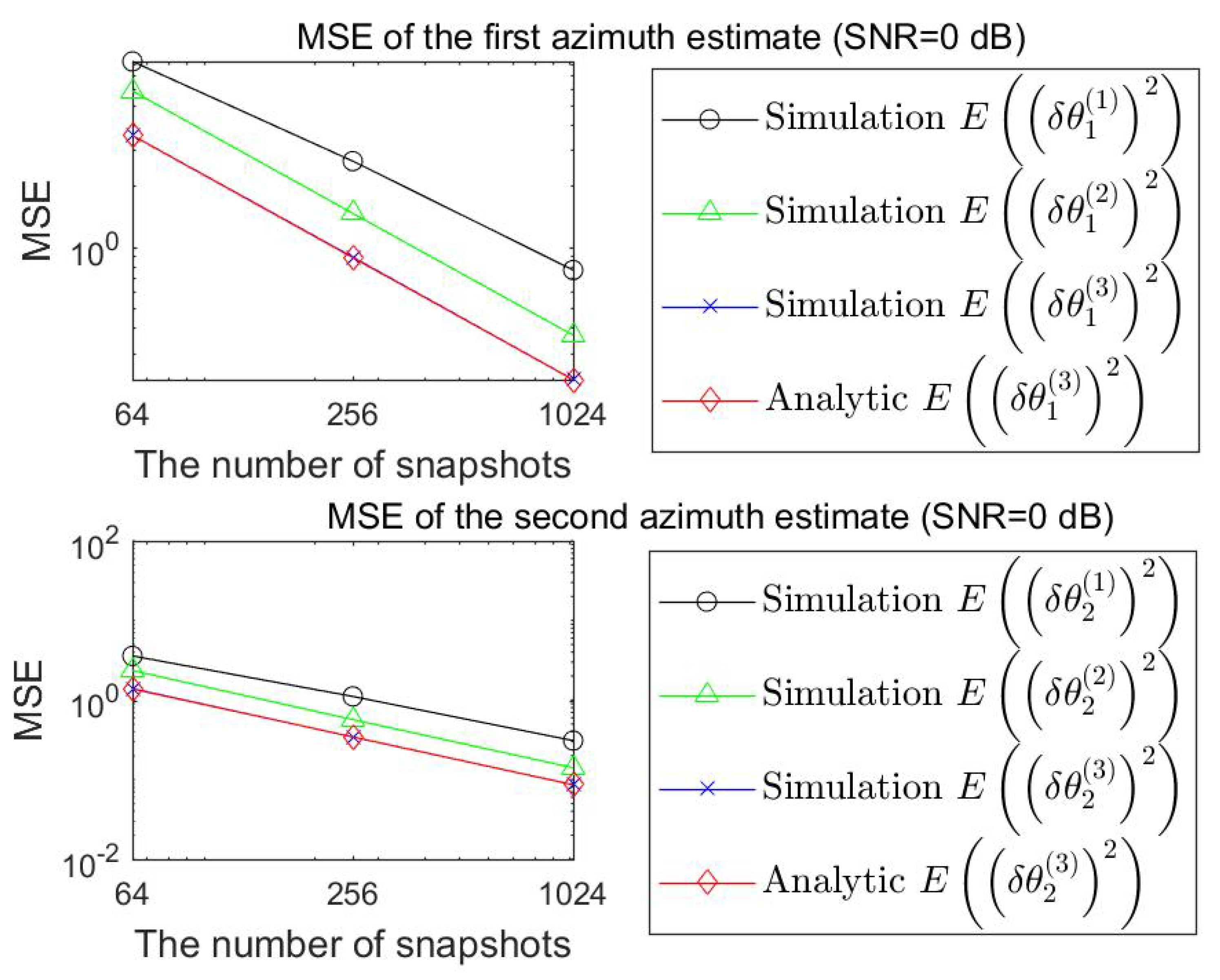
Figure 3, Figure 4 and Figure 5 illustrate how MSEs are dependent on the number of snapshots for the fixed number of repetitions of 10,000. It is clearly shown that MSEs for all the estimates improve as the number of snapshots increases. It is illustrated that the empirical MSEs with respect to the number of snapshots of δ θ 1 2 and δ θ 1 3 are close to that of δ θ 1 1 . In the upper plot of Figure 3, it is clear that the agreement between empirical MSE of δ θ 1 ( 3 ) , and analytic MSE of δ θ 1 ( 3 ) improves as the number of snapshots increases, which is quite reasonable. The same is true for the upper plots of the Figure 4 and Figure 5. The above observations for the MSEs are illustrated in the lower plots of Figure 3, Figure 4 and Figure 5, where the MSEs of the second incident signal are shown.
In Figure 3, Figure 4 and Figure 5, we illustrate how small the MSEs of δ θ n ( 1 ) , δ θ n ( 2 ) and δ θ n ( 3 ) are. The results with “Simulation E δ θ n ( 1 ) 2 ”, “Simulation E δ θ n ( 2 ) 2 ”, and “Simulation E δ θ n ( 3 ) 2 ” are obtained from (48), (49), and (50), respectively.
In Figure 3, Figure 4 and Figure 5, the agreement between the simulation results with superscript (3) and the analytic results improves as the number of snapshots increases, since the analytic results are essentially based on ensemble-average, and the simulation results are based on time-average. Therefore, the agreement between the simulation results and the analytic results should be checked for large number of snapshots.
In Figure 3, Figure 4 and Figure 5, the agreement between the simulation results with superscript (1) and the analytic results is not as good as that between the simulation results with superscript (3) and the analytic results, since the analytic results are associated with the simulation results with superscript (3). Similarly, the agreement between the simulation results with superscript (2) and the analytic results is not as good as that between the simulation results with superscript (3) and the analytic results.
Figure 6, Figure 7 and Figure 8 illustrate how the MSEs are dependent on the number of repetitions for the fixed number of snapshots of 1024. It is clearly shown that the MSEs for all the estimates improve as the number of repetitions increases. It is shown in Figure 6, Figure 7 and Figure 8 that the agreements between analytic results and simulation results with superscript (3) are quite good for the number of repetitions of 10,000. Note that the number of repetitions in the Monte–Carlo simulation should be large enough for the simulation-based MSEs to be reliable.

9. Applications of Derived Analytic Expression of MSE of the MUSIC Algorithm

9.1. Evaluation of cOvariance Matrix of AOA-Based Localization in Underwater Acoustics

Once the sound source is detected, localization can be applied to pinpoint the location of an emitter. AOA-based localization can be adopted in this stage. Sensor locations and line-of-bearings (LOBs) from DOA estimation algorithm should be available to implement AOA-based localization algorithm. Any DOA estimation algorithm, including the MUSIC, the maximum-likelihood (ML), the conventional beamforming, the Capon beamforming, can be employed to get the LOBs used for localization. Note that the mean-square-error (MSE) of the location estimation algorithm is highly dependent on the MSE of the DOA estimation algorithm, which implies that, for accurate localization of an emitter location, the MSE of the DOA estimation algorithm should be small. The accuracy of the localization algorithm is quantified in terms of the covariance matrix of the position error δ r [29]:
E δ r δ r T = H # Λ H # T
where H and Λ are defined from
Λ = σ 1 2 d 1 2 0 0 σ N 2 d N 2
H = sin θ 1 0 cos θ 1 0 sin θ N 0 cos θ N 0 .
The superscript # in (51) denotes a pseudo inverse operator. Note that σ i , d i in (52) and θ i 0 in (53) are standard deviation of the DOA estimate at the i-th sensor location, the distance from the i–th sensor location to an emitter, and true DOA at i-th sensor location, respectively. For an unbiased DOA estimator, θ i 0 can be obtained from the square root of the MSE of DOA estimate.
If the MUSIC algorithm is employed to get DOA estimate, the MSE of the estimate in (40) can be used for calculation of σ i in (52).

9.2. Evaluating the Performance of Ultrasonic Imaging

In [30], the MUSIC algorithm for DOA estimation is considered. Basically, the MUSIC algorithm is super resolution algorithm in that it can resolve closely spaced signals, Super resolution in the ultrasonic imaging is very important: Whether two closely located objects can be resolved or not is highly dependent on the resolution of the adopted imaging algorithm. Therefore, the MUSIC algorithm can be a good candidate for ultrasonic imaging. In, the authors derived the expression of the resolution, which is a measure of resolving capability of two closely located objects. Although, in [30], the explicit expression of the resolution is derived, the explicit expression of the estimation accuracy is not presented, and the derived explicit expression of the MSE of the MUSIC algorithm can be used to evaluate the MSE of the MUSIC-based estimates. Therefore, the difference between [30] and this paper is that the resolution is evaluated in [30] and the MSE is evaluated in this paper. In imaging, usually, resolving two closely-spaced objects is important, which is why many studies on derivation of the expression of the resolution of the MUSIC algorithm have been conducted. Absolute peak location can also be important in some ultrasonic imaging when the estimation of the exact location of the object is important. In that case, the MSE should be obtained to quantify the accuracy of the peak location in the MUSIC-based imaging.
The peak location of the MUSIC algorithm-based imaging corresponds to the location of an object, and the MSE implies how close the estimated location is to the true location of the object.

9.3. Evaluation of Ranging Accuracy in the MUSIC-Based Laser Ranging Algorithm in Terms of the Mean Square Error

In [31], the authors proposed to apply the MUSIC algorithm in range estimation for use with frequency-modulated continuous wave (FMCW) laser. Traditionally, the fast Fourier transform (FFT) is for ranging. For improvement of ranging accuracy via the super resolution property of the MUSIC algorithm, the MUSIC algorithm can be employed for frequency estimation. The ranging accuracy in terms of the mean square error can be obtained from (40) of this paper if the laser measurement noise can be modelled as an additive Gaussian noise.

9.4. Localization Accuracy in the MUSIC Algorithm for Use With Super Resolution Fluorescence Microscopy

The authors in [32] propose a new algorithm called MUSICAL which is a modified version of the classical MUSIC algorithm. The MUSICAL is proposed to solve a few problems in the classical MUSIC algorithm. Although the authors show that the MUSICAL algorithm outperforms the conventional MUSIC algorithm, they do not derive an explicit expression of the MSE of the distance estimate for the MUSICAL algorithm. The derivation leading to (40) in this paper can be modified to derive the expression of the MSE of the MUSICAL algorithm. The modification should reflect the difference between the MUSICAL algorithm and the MUSIC algorithm.

9.5. Accuracy in the MUSIC-Based Scattering Center Estimation

One of popular remote sensing sensors is radar. In radar target recognition, range profile of a radar target is a good feature vector in that the peaks of a range profile correspond to scattering centers of the radar target. For a specific aspect angle, the distance between each peak location of range profile and true location of scattering center can be defined as estimation accuracy. Traditionally, the FFT is used to get the range profile. In [33], the authors employ the MUSIC algorithm to get range profile. Although the authors proposed a new MUSIC-based scheme to get range profile, which is superior to the conventional FFT-based scheme, they did not present an expression of the MSE associated with the estimate obtained from the peaks of the MUSIC-based range profile. By modifying the derivation leading to (40), the MSE of the estimate from MUSIC-based range profile can be obtained. The modification should reflect how the MUSIC algorithm for generation of the range profile is different from the original MUSIC algorithm for generation of DOA spectrum.

10. Conclusions

Based on some approximations and the Taylor series expansion, we have derived a few expressions of an approximation of estimate of the MUSIC algorithm. The estimates are obtained by approximating the signal eigenvector and the projection matrix onto the column space of the eigenvector matrix. Two closed-form expressions of the DOA estimate have been derived by applying two approximations. For one of two expressions, closed-form expression of the MSE of the estimate as well as the closed-form of the estimate itself have been derived. The closed-form expression of the MSE has been validated by comparing it with empirically obtained MSE. The derived expression of the MSE of the estimates can be used for the performance analysis of the MUSIC algorithm. From the viewpoint of the computational complexity, an analytic MSE of the estimate can be evaluated much more easily in comparison with an empirical MSE from the time-consuming Monte–Carlo simulation.
The proposed scheme can be used for the performance analysis in predicting how accurate the estimate of the MUSIC algorithm is without resorting computationally intensive Monte–Carlo simulation. The performance of the MUSIC algorithm is dependent on various parameters, such as the number snapshots, the number antenna elements in the array, inter-element spacing between adjacent antenna elements and the SNR. Therefore, making Monte–Carlo simulations for different values of the various parameters is computationally very intensive, and the analytic performance analysis proposed in this paper can be employed to predict how well the MUSIC algorithm works, given the specific values of the parameters.

Author Contributions

S.-H.J. mainly made a matlab implementation of the proposed algorithm. J.-H.L. formulated the proposed algorithm. J.-H.L. and S.-H.J. wrote an initial draft. B.-K.S. and S.-H.J. derived the results in the appendices. B.-K.S. helped S.-H.J. make a numerical implementation of the proposed algorithm. All authors have read and agreed to the published version of the manuscript.

Funding

The authors gratefully acknowledge the support from Electronic Warfare Research Center at Gwangju Institute of Science and Technology (GIST), originally funded by Defense Acquisition Program Administration (DAPA) and Agency for Defense Development (ADD). This work was partially supported by Electronics and Telecommunications Research Institute (ETRI) grant funded by the korean government [20ZD1110, Development of ICT Convergence Technology for Daegu-GyeongBuk Regional Industry].

Conflicts of Interest

The authors declare no conflict of interest.

Appendix A. Calculation of E δ R k l R δ R k l C *

From (12) and (13), E δ R k l R δ R k l C * can be rewritten as
E δ R k l R δ R k l C * = E δ R k l R δ R k l C * ,
since, from (13), δ R k l C is not stochastic when the noise is zero-mean Gaussian distributed, E δ R k l R is expressed as
E δ R k l R = 1 L i = 1 L σ 2 δ k l , δ k l = 1 k = l 0 k l .

Appendix B. Calculation of E δ R k l C δ R k l R *

From (12) and (13), E δ R k l C δ R k l R * can be rewritten as
E δ R k l C δ R k l R * = δ R k l C E δ R k l R * ,
since, from (13), δ R k l C * is deterministic. E δ R k l R * is expressed as
E δ R k l R * = 1 L i = 1 L σ 2 δ k l ,
where δ k l is defined as
δ k l = 1 k = l 0 k l .

Appendix C. Calculation of E δ R k l C δ R k l C *

Since δ R k l C is deterministic, not stochastic, E δ R k l C δ R k l C * is given by
E δ R k l C δ R k l C * = δ R k l C δ R k l C * .

References

  1. Schmidt, R. Multiple emitter location and signal parameter estimation. IEEE Trans. Antennas Propag. 1986, 34, 276–280. [Google Scholar] [CrossRef] [Green Version]
  2. Stoica, P.; Nehorai, A. MUSIC, maximum likelihood, and Cramer-Rao bound. IEEE Trans. Acoust. Speech Signal Process. 1989, 37, 720–741. [Google Scholar] [CrossRef]
  3. Krim, H.; Viberg, M. Two decades of array signal processing research: The parametric approach. IEEE Signal Process. Mag. 1996, 13, 67–94. [Google Scholar] [CrossRef]
  4. Kaveh, M.; Barabell, A. The statistical performance of the MUSIC and the minimum-norm algorithms in resolving plane waves in noise. IEEE Trans. Acoust. Speech Signal Process. 1986, 34, 331–341. [Google Scholar] [CrossRef]
  5. Jeffries, D.; Farrier, D. Asymptotic results for eigenvector methods. IEE Proc. F-Commun. Radar Signal Process. 1985, 132, 589–594. [Google Scholar] [CrossRef]
  6. Ferreol, A.; Larzabal, P.; Viberg, M. On the asymptotic performance analysis of subspace DOA estimation in the presence of modeling errors: Case of MUSIC. IEEE Trans. Signal Process. 2006, 54, 907–920. [Google Scholar] [CrossRef]
  7. Zhang, Q. Probability of resolution of the MUSIC algorithm. IEEE Trans. Signal Process. 1995, 43, 978–987. [Google Scholar] [CrossRef]
  8. Swindlehurst, A.L.; Kailath, T. A performance analysis of subspace-based methods in the presence of model errors, Part I: The MUSIC algorithm. IEEE Trans. Signal Process. 1992, 40, 1758–1774. [Google Scholar] [CrossRef]
  9. Stoica, P.; Nehorai, A. MUSIC, maximum likelihood, and Cramer-Rao bound: Further results and comparisons. IEEE Trans. Acoust. Speech Signal Process. 1990, 38, 2140–2150. [Google Scholar] [CrossRef]
  10. Pillai, S.U.; Kwon, B.H. Performance analysis of MUSIC-type high resolution estimators for direction finding in correlated and coherent scenes. IEEE Trans. Acoust. Speech Signal Process. 1989, 37, 1176–1189. [Google Scholar] [CrossRef]
  11. Cho, Y.S.; Seo, J.M.; Lee, J.H. Performance analysis of two-dimensional maximum likelihood direction-of-arrival estimation algorithm using the UCA. Int. J. Antennas Propag. 2017, 2017, 6926825. [Google Scholar] [CrossRef] [Green Version]
  12. Wang, M.; Zhang, Z.; Nehorai, A. Performance analysis of coarray-based MUSIC in the presence of sensor location errors. IEEE Trans. Signal Process. 2018, 66, 3074–3085. [Google Scholar] [CrossRef]
  13. Wang, B.; Gu, Y.; Wang, W. Off-grid direction-of-arrival estimation based on steering vector approximation. Circuits Syst. Signal Process. 2019, 38, 1287–1300. [Google Scholar] [CrossRef]
  14. Vincent, F.; Pascal, F.; Besson, O. A bias-compensated MUSIC for small number of samples. Signal Process. 2017, 138, 117–120. [Google Scholar] [CrossRef] [Green Version]
  15. Liu, B.; Gui, G.; Matsushita, S.; Xu, L. Dimension-reduced direction-of-arrival estimation based on 2,1-norm penalty. IEEE Access 2018, 6, 44433–44444. [Google Scholar] [CrossRef]
  16. Vallet, P.; Mestre, X.; Loubaton, P. Performance analysis of an improved MUSIC DoA estimator. IEEE Trans. Signal Process. 2015, 63, 6407–6422. [Google Scholar] [CrossRef] [Green Version]
  17. An, D.J.; Lee, J.H. Performance analysis of amplitude comparison monopulse direction-of-arrival estimation. Appl. Sci. 2020, 10, 1246. [Google Scholar] [CrossRef] [Green Version]
  18. Lin, Y.; Guo, T.; Guo, M.; Fu, Y. Motion compensation for SAA FMCW radar based on specific switching scheme. Appl. Sci. 2019, 9, 3441. [Google Scholar] [CrossRef] [Green Version]
  19. Wang, F.; Chen, Y.; Wan, J. In-depth exploration of signal self-cancellation phenomenon to achieve DOA estimation of underwater acoustic sources. Appl. Sci. 2019, 9, 570. [Google Scholar] [CrossRef] [Green Version]
  20. Wang, Z.; Li, J.; Yan, Y. Target speaker localization based on the complex watson mixture model and time-frequency selection neural network. Appl. Sci. 2018, 8, 2326. [Google Scholar] [CrossRef] [Green Version]
  21. Zou, Y.; Liu, Z.; Ritz, C.H. Enhancing target speech based on nonlinear soft masking using a single acoustic vector sensor. Appl. Sci. 2018, 8, 1436. [Google Scholar] [CrossRef] [Green Version]
  22. Tomic, S.; Beko, M.; Camarinha-Matos, L.M.; Oliveira, L.B. Distributed localization with complemented RSS and AOA measurements: Theory and Methods. Appl. Sci. 2020, 10, 272. [Google Scholar] [CrossRef] [Green Version]
  23. Yagüe-Jiménez, V.; Ibáñez Rodríguez, A.; Parrilla Romero, M.; Martínez-Graullera, O. Rician beamforming: Despeckle method via coarray projection stochastic analysis. Appl. Sci. 2020, 10, 847. [Google Scholar] [CrossRef] [Green Version]
  24. Mohamed, K.S.; Alias, M.Y.; Roslee, M. Interference avoidance using TDMA-beamforming in location aware small cell systems. Appl. Sci. 2019, 9, 4979. [Google Scholar] [CrossRef] [Green Version]
  25. Gadiel, G.M.; Lee, K. Energy-efficient hybrid beamforming with variable and constant phase shifters. Appl. Sci. 2019, 9, 4476. [Google Scholar] [CrossRef] [Green Version]
  26. Xie, J.; Li, X.; Xing, Z.; Zhang, B.; Bao, W.; Zhang, J. Improved distributed minimum variance distortionless response (MVDR) beamforming method based on a local average consensus algorithm for bird audio enhancement in wireless acoustic sensor networks. Appl. Sci. 2019, 9, 3153. [Google Scholar] [CrossRef] [Green Version]
  27. Golub, G.H.; Van Loan, C.F. Matrix Computations; Johns Hopkins University Press: Baltimore, MD, USA, 2012; Volume 3. [Google Scholar]
  28. Burden, R.L.; Faires, J.D. Numerical Analysis; Cengage Learning Press: Boston, MA, USA, 2010; Volume 9. [Google Scholar]
  29. Pages-Zamora, A.; Vidal, J.; Brooks, D.H. Closed-form solution for positioning based on angle of arrival measurements. In Proceedings of the 13th IEEE International Symposium on Personal, Indoor and Mobile Radio Communications, Pavilhao Altantico, Lisboa, Portugal, 18 September 2002; Volume 4, pp. 1522–1526. [Google Scholar]
  30. Fan, C.; Caleap, M.; Pan, M.; Drinkwater, B.W. A comparison between ultrasonic array beamforming and super resolution imaging algorithms for non-destructive evaluation. Ultrasonics 2014, 54, 1842–1850. [Google Scholar] [CrossRef] [Green Version]
  31. Pan, H.; Zhang, F.; Shi, C.; Qu, X. High-precision frequency estimation for frequency modulated continuous wave laser ranging using the multiple signal classification method. Appl. Opt. 2017, 56, 6956–6961. [Google Scholar] [CrossRef]
  32. Agarwal, K.; Macháň, R. Multiple signal classification algorithm for super-resolution fluorescence microscopy. Nat. Commun. 2016, 7, 1–9. [Google Scholar] [CrossRef] [Green Version]
  33. Kim, K.T.; Seo, D.K.; Kim, H.T. Efficient radar target recognition using the MUSIC algorithm and invariant features. IEEE Trans. Antennas Propag. 2002, 50, 325–337. [Google Scholar]
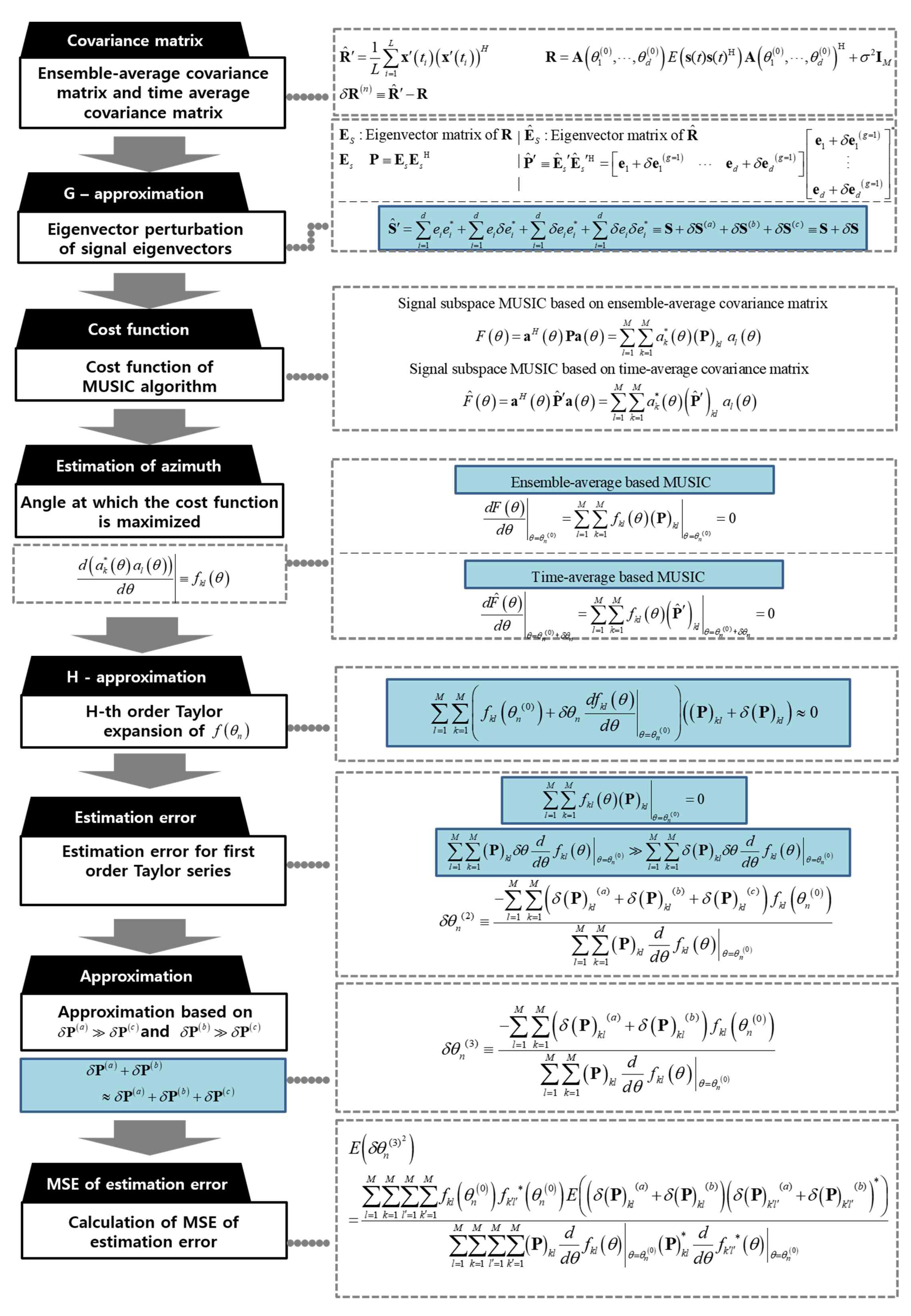
Figure 1. Summary of performance analysis of the multiple signal classification (MUSIC) algorithm.
Applsci 10 02063 g001
Figure 2. Difference between the existing method and the proposed scheme.
Applsci 10 02063 g002
Figure 3. Mean square error of δ θ with respect to the number of snapshots (SNR = −10 dB).
Applsci 10 02063 g003
Figure 4. Mean square error of δ θ with respect to the number of snapshots (SNR = 0 dB).
Applsci 10 02063 g004
Figure 5. Mean square error of δ θ with respect to the number of snapshots (SNR = 10 dB).
Applsci 10 02063 g005
Figure 6. Mean square error of δ θ with respect to the number of repetitions (SNR = −10 dB).
Applsci 10 02063 g006
Figure 7. Mean square error of δ θ with respect to the number of repetitions (SNR = 0 dB).
Applsci 10 02063 g007
Figure 8. Mean square error of δ θ with respect to the number of repetitions (SNR = 10 dB).
Applsci 10 02063 g008
Table 1. Algorithms, applications, main ideas and contributions of the recently published works on direction-of-arrival (DOA) estimation and beamforming.
Ref.AlgorithmApplicationMain IdeaContribution
[17]Amplitude comparison monopulse DOA estimationRadar trackingAnalytic performance analysisComputationally inexpensive performance analysis
[18]Conventional beamforming (Bartlett beamforming) algorithmFMCW automotive radarMotion compensated Bartlett beamformingEstimation error reduction by explicitly taking the motion induced phase into account
[19]MVDR beamforming-based DOA algorithmDOA of underwater acoustic sourcesSignal self-cancellation MVDRPerformance improvement of MVDR algorithm for underwater acoustic source localization
[20]New DOA estimation algorithm based on Complex Watson mixture model and time-frequency selectionAcoustic source localizationIsolation of target speaker by time-frequency selectionPerformance improvement of DOA estimation of target speaker
[21]DOA estimation with acoustic vector sensor (AVS): Preprocessing for target speech enhancementEnhancement of target speechEstimated DOA-based isolation of target speech in time-frequency distribution for enhancementSuperiority of AVS-SMASK over AVS-FMV
[22]Array signal processing-based DOA estimation algorithms using array antennas and DOA estimation using single directional antennaAOA-based localizationNot applicable [Review paper]Not applicable [Review paper]
[23]Rician beamforming for array design [Not beamforming-based DOA estimation algorithm]Ultrasonic imagingRician beamforming-based array design for ultrasonic imaging using convex optimizationImproved despeckle in ultrasonic imaging via beamforming-based array design
[24]TDMA-beamforming for array design [Not beamforming-based DOA estimation algorithm]Interference suppression in communication systemInterference suppression via spatial filteringImproved interference avoidance
[25]Hybrid beamforming for array design [Not beamforming-based DOA estimation algorithm]Massive MIMO systemOptimal combination of variable phase shifters and constant phase shiftersImprovement in beamforming performance
[26]MVDR beamforming for array design [Not beamforming-based DOA estimation algorithm]Bird audio enhancementBeamforming method based on a local average consensus algorithmEfficient implementation of acoustic wireless sensor network for surveillance
Table 2. How to validate the schemes presented in [17,18,19,20,21,22,23,24,25,26], and how to apply the derivations of this paper to the problems in [17,18,19,20,21,22,23,24,25,26].
Ref.How to Validate the Schemes Presented in [17,18,19,20,21,22,23,24,25,26]How to Apply the Derivations of This Paper to the Problems in [17,18,19,20,21,22,23,24,25,26]
[17]Agreement between analytic MSE and simulation-based MSE[17]: Performance analysis of amplitude comparison monopulse algorithm. This paper: Performance analysis of the MUSIC algorithm
[18]Reduction in estimation error of the motion compensated conventional beamforming algorithm in comparison with the estimation error of original conventional beamforming algorithm without motion compensation in the DOA spectrumThe analytic expression of the MSE of motion-compensated Bartlett beamforming algorithm can be obtained by modifying the derivation in this paper
[19]Superiority of performance of SCC-MVDR algorithm over MVDR algorithm in the view point of RMSEThe analytic expression of the MSE of SCC-MVDR algorithm can be obtained by modifying the derivation in this paper
[20]Superiority of the proposed scheme over the previously existing algorithms in terms of gross error rate (GER) and mean square error (MSE)Performance of the proposed algorithm in terms of the MSE can be analytically obtained by modifying the derivation in this paper
[21]Performance comparison in terms of signal-to-noise ratio, signal-to-interference ratio, signal-to-interference ratio, signal-to-interference plus noise ratio, log spectral density, and perceptual evaluation of speech qualityPerformance of preprocessing DOA estimation with AVS algorithm, given by estimation error, can be obtained by modifying the derivation leading to (38) and (39), since the derivation of the MUSIC estimate should be modified to the derivation of the AVS-based DOA estimate
[22]Not applicable [Review paper]Performance of AOA-based localization algorithm depends on performance of DOA estimation: The MSE of the MUSIC algorithm can be obtained from (40) of this paper. The MSE of other DOA estimation algorithm can be obtained by modifying the derivation leading to (40).
[23]Comparison of images in terms of quality and localized estimations on image noiseRician beamforming-based array design is formulated as a convex optimization problem, and the MSEs of the array design parameters can be analytically obtained by modifying the derivation leading to (40) since array design can be formulated as parameter estimation problem
[24]Superiority of the proposed scheme in terms of throughput, Jain’s fairness model, and SINR.The MSEs of the estimated array parameters in array design problem can be analytically derived by modifying the approach leading to (40).
[25]Superiority of the proposed algorithm in terms of average sum-rate and energy efficiencyThe MSEs of the estimates in hybrid beamforming based array design can be evaluated by modification of the derivation leading to (40).
[26]Improvement in MSE, SegSNR and PESQThe MSE of the estimated array design parameters can be evaluated by modification of the derivation leading to (40).