Performance Characteristics of an Orthopter-Type Vertical Axis Wind Turbine in Shear Flows

Abstract
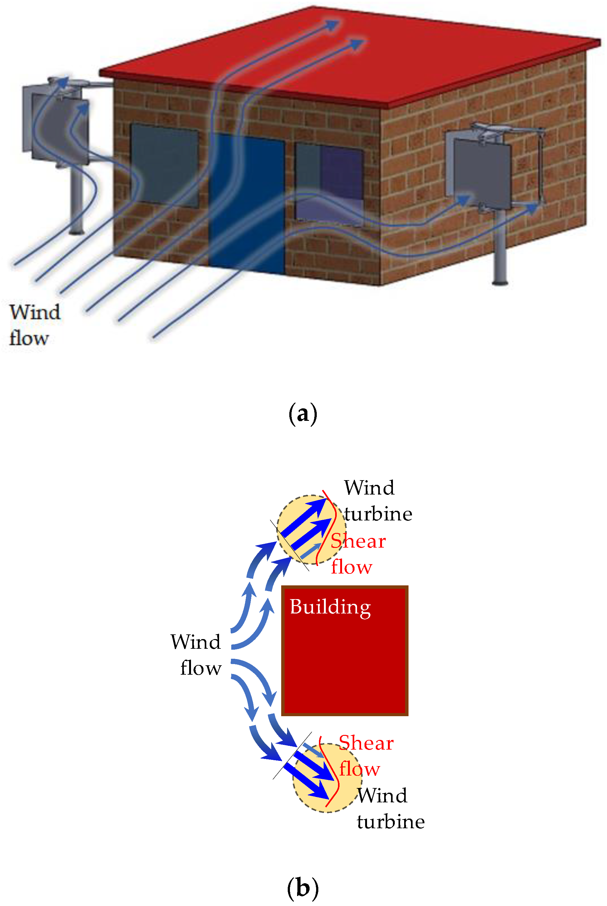
1. Introduction
2. Experimental Approach
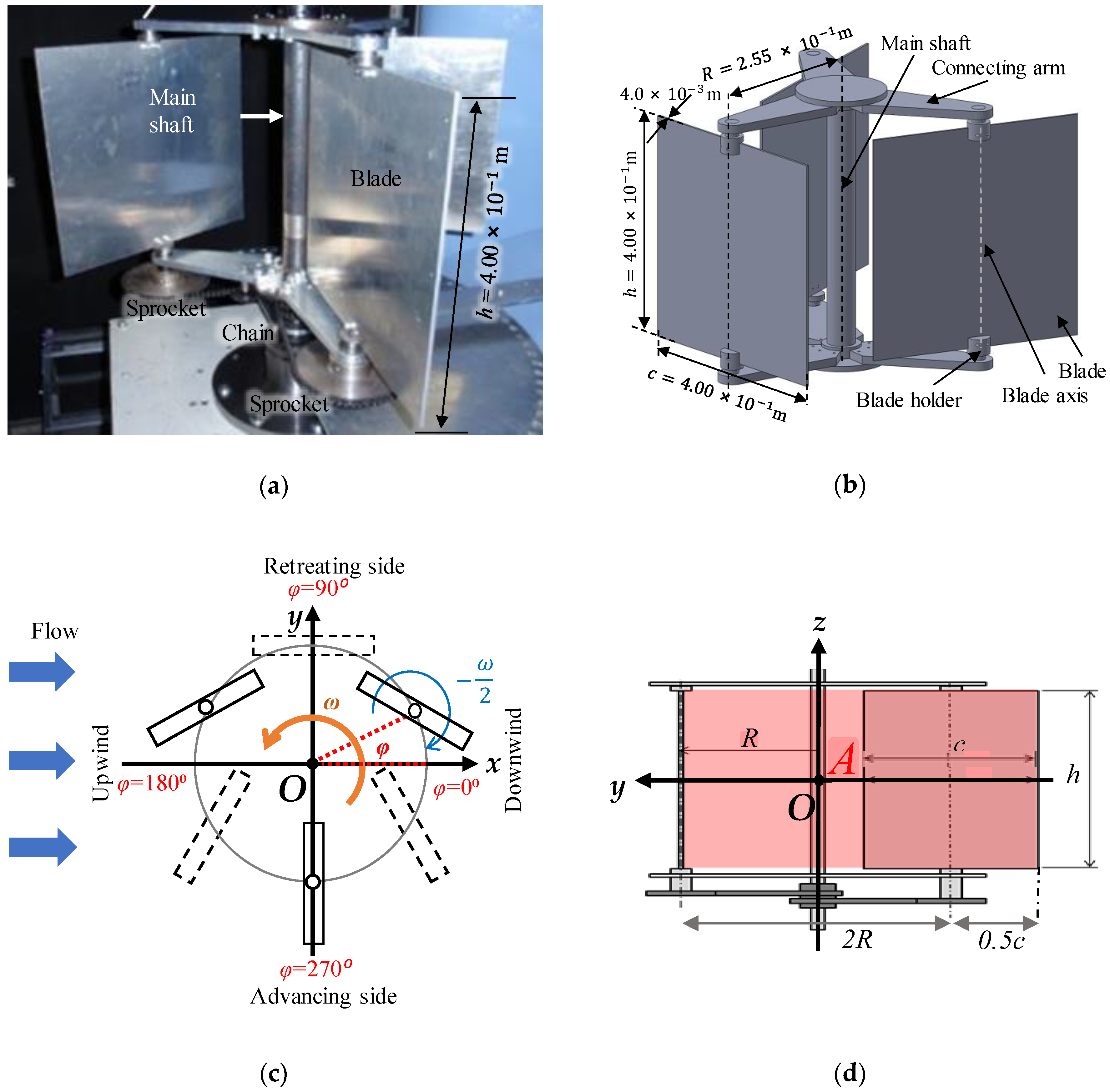
2.1. Wind Turbine Model
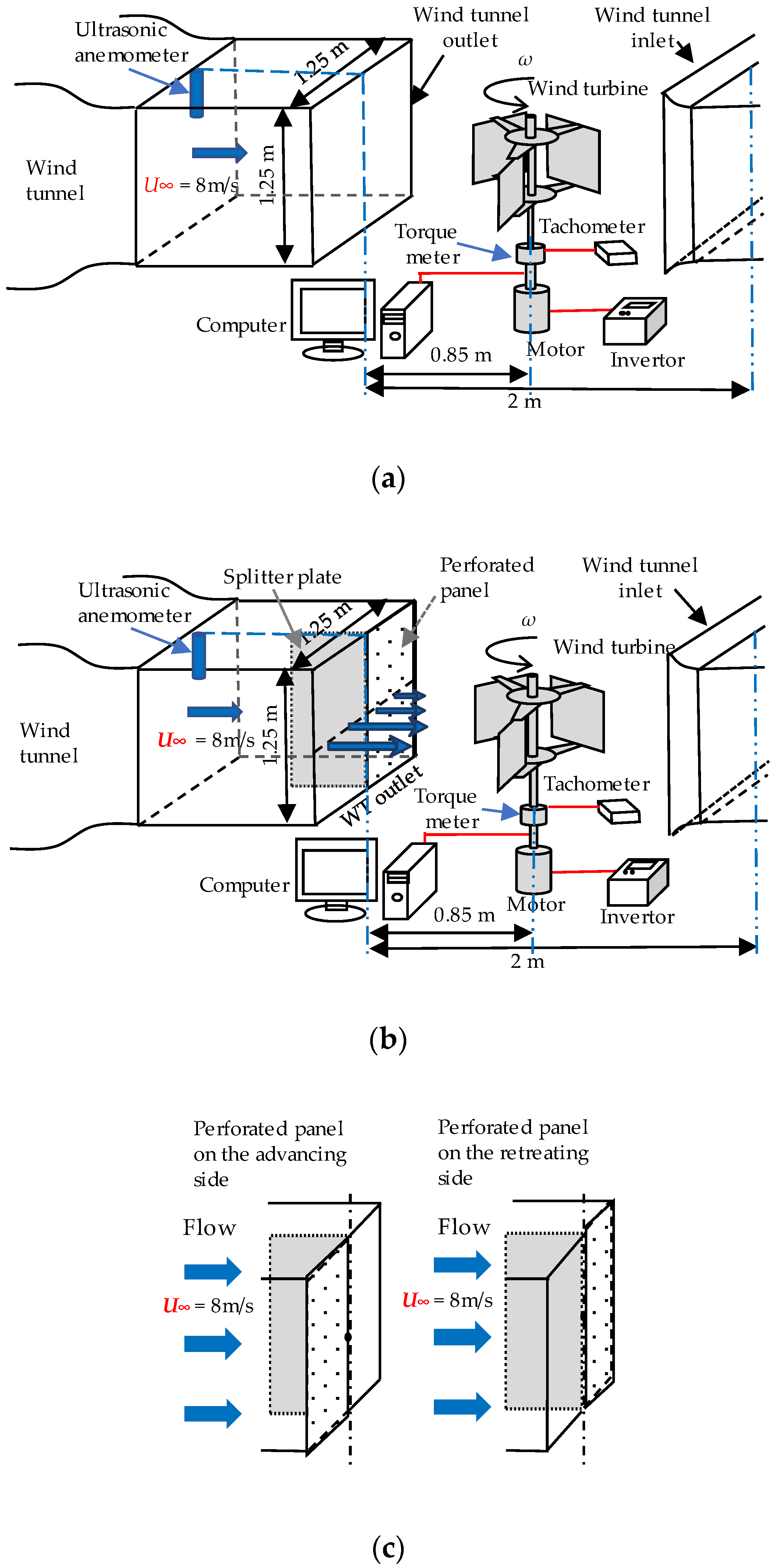
2.2. Experimental Setup for Uniform Flow Case
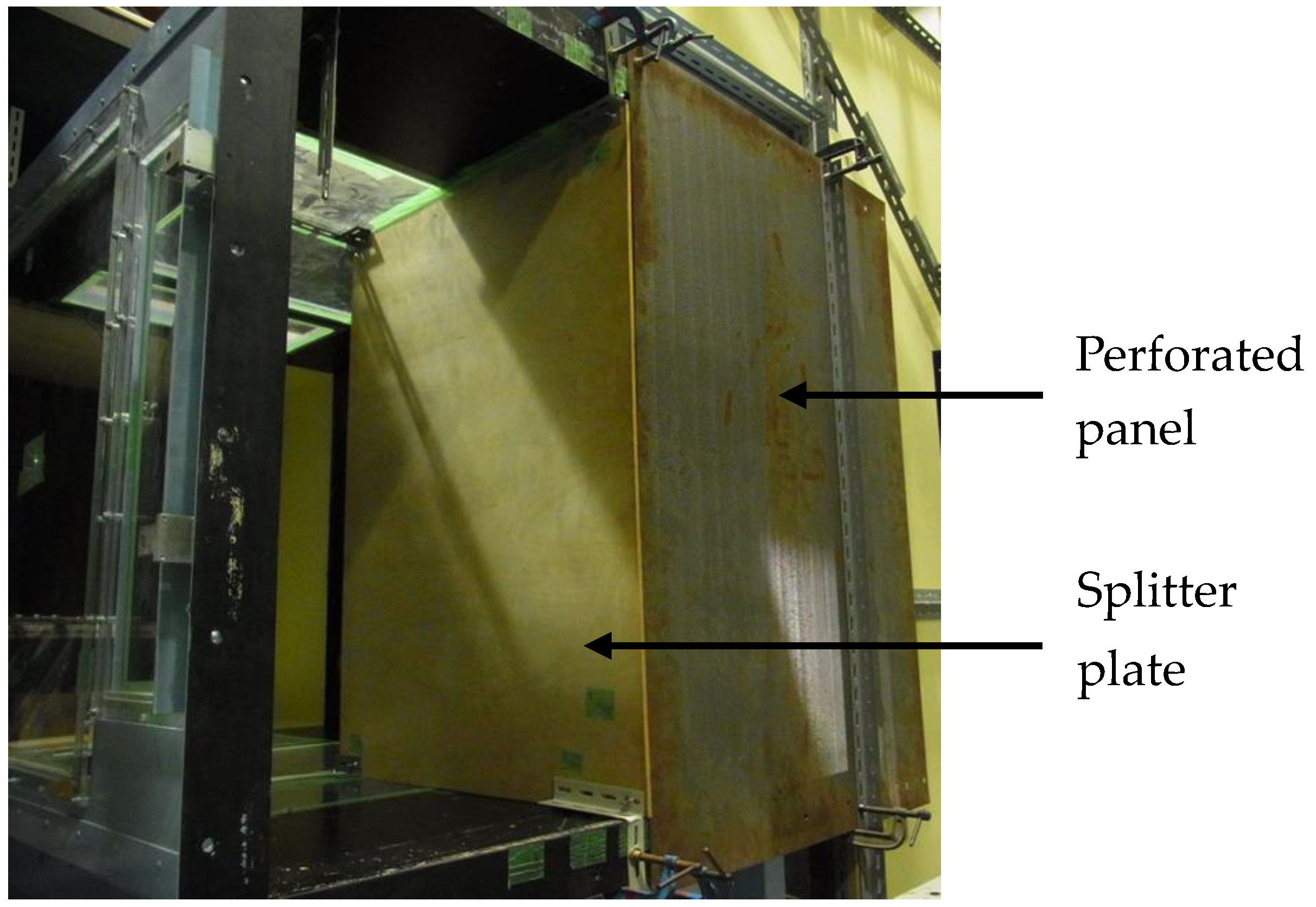
2.3. Experimental Setup for Shear Flow Cases
2.4. Torque and Power Coefficients
3. Numerical Approach
3.1. Governing Equations and Discretization Method
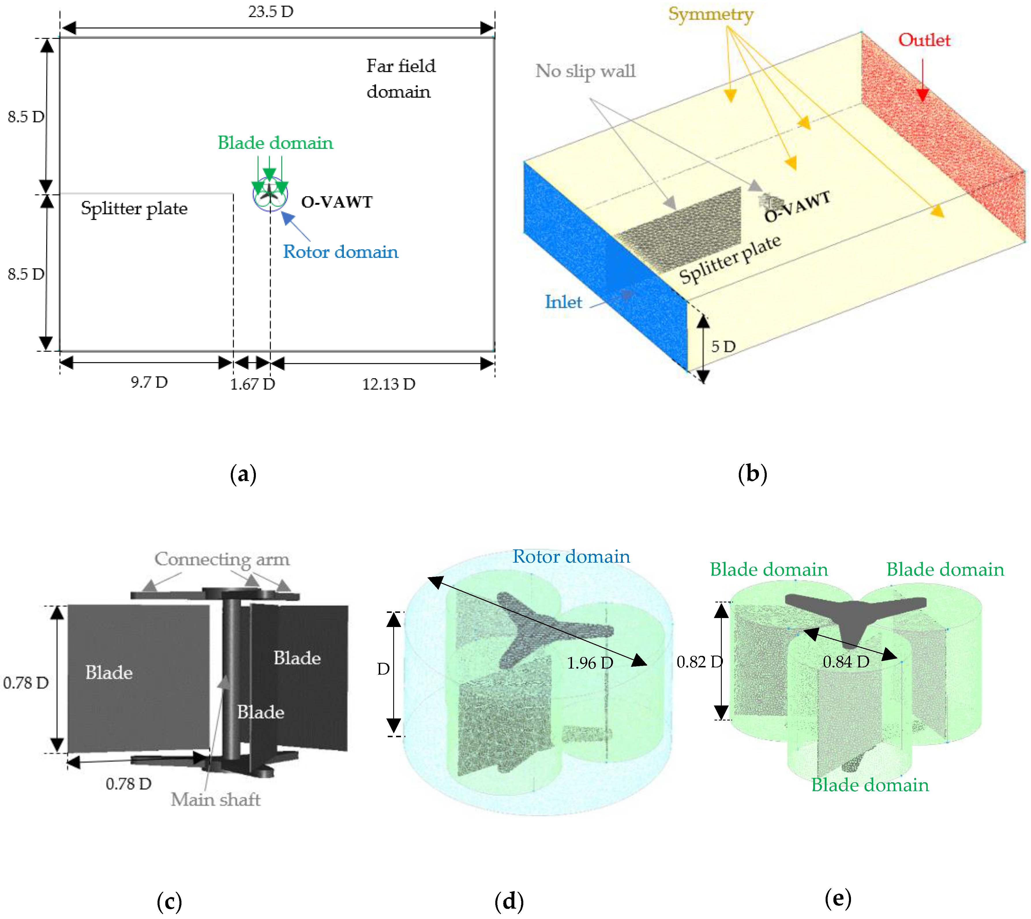
3.2. Numerical Setup
3.3. Torque and Power Coefficients
4. Results and Discussion
4.1. Performance in Uniform Flow
4.2. Performance in Shear Flows
4.3. Flow Characteristics
5. Conclusions
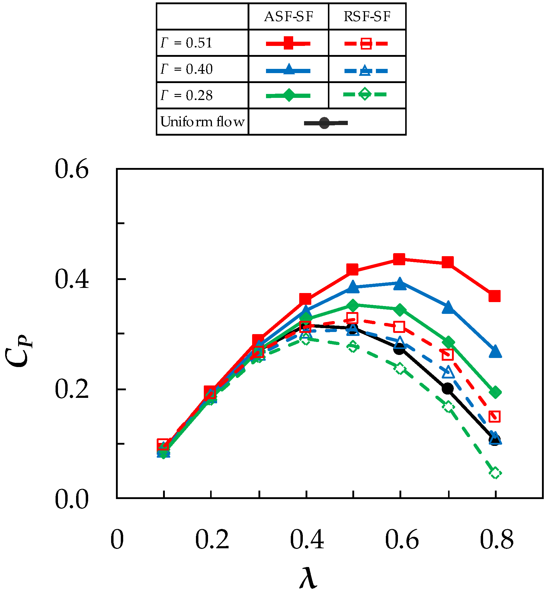
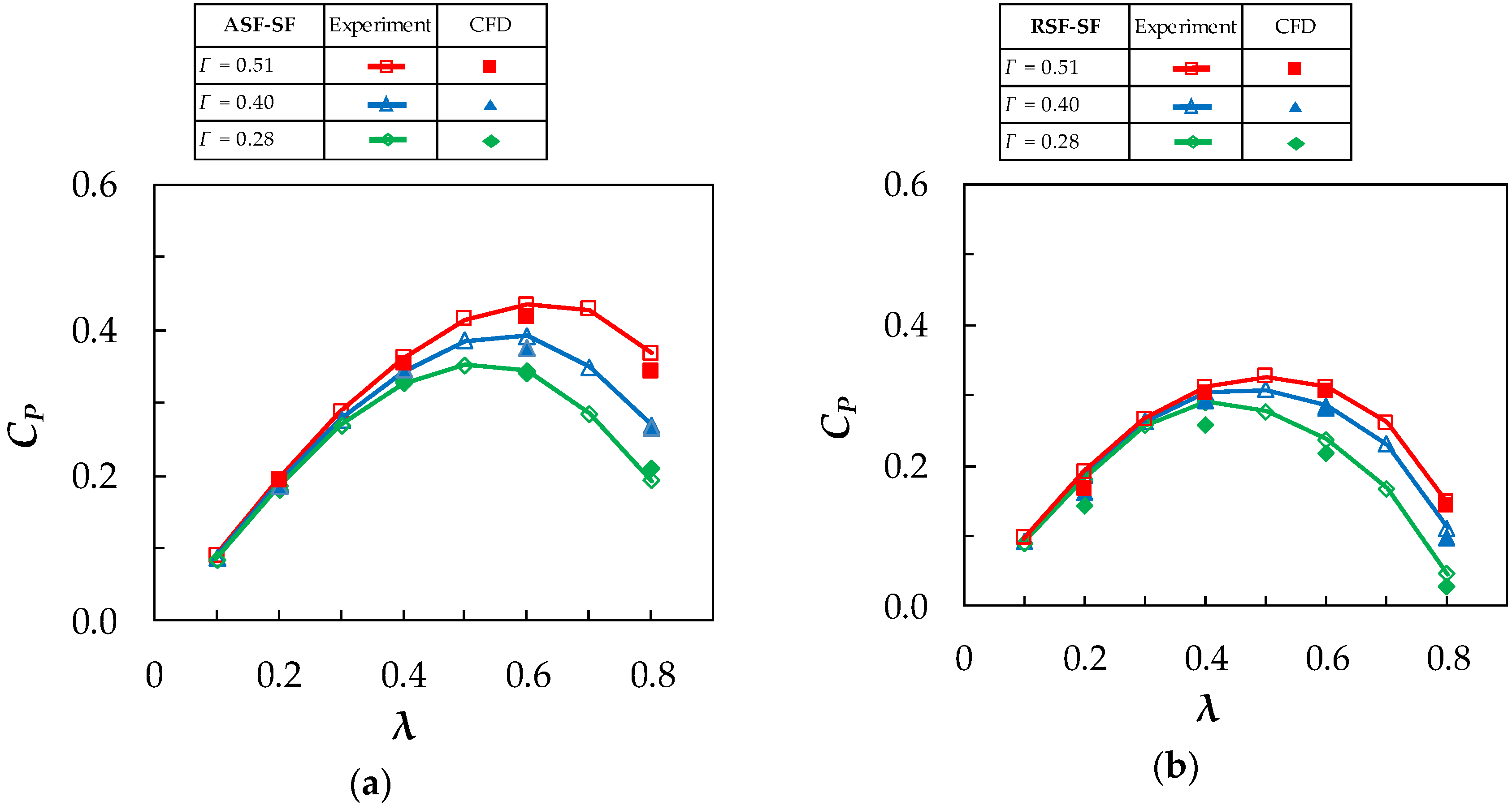
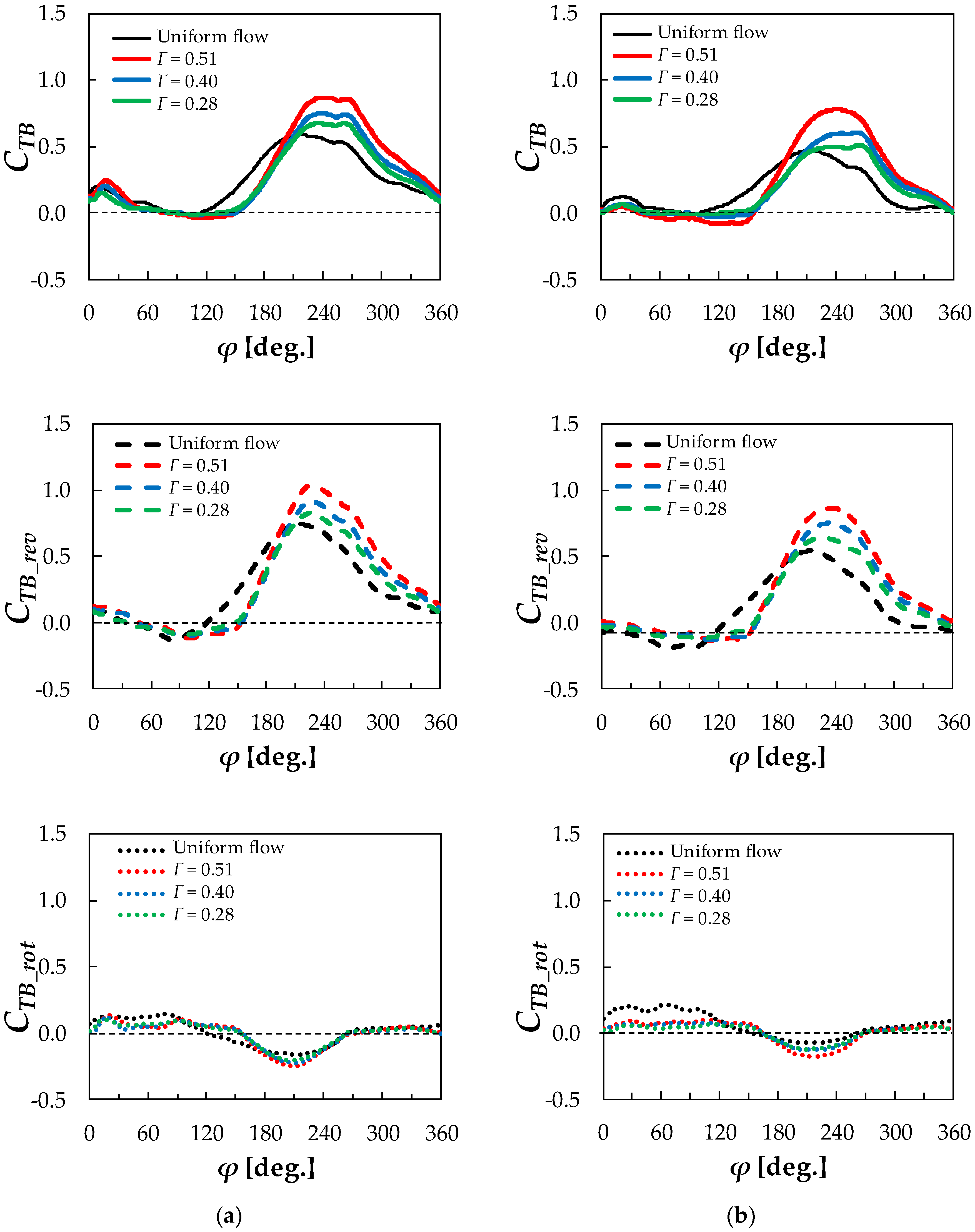
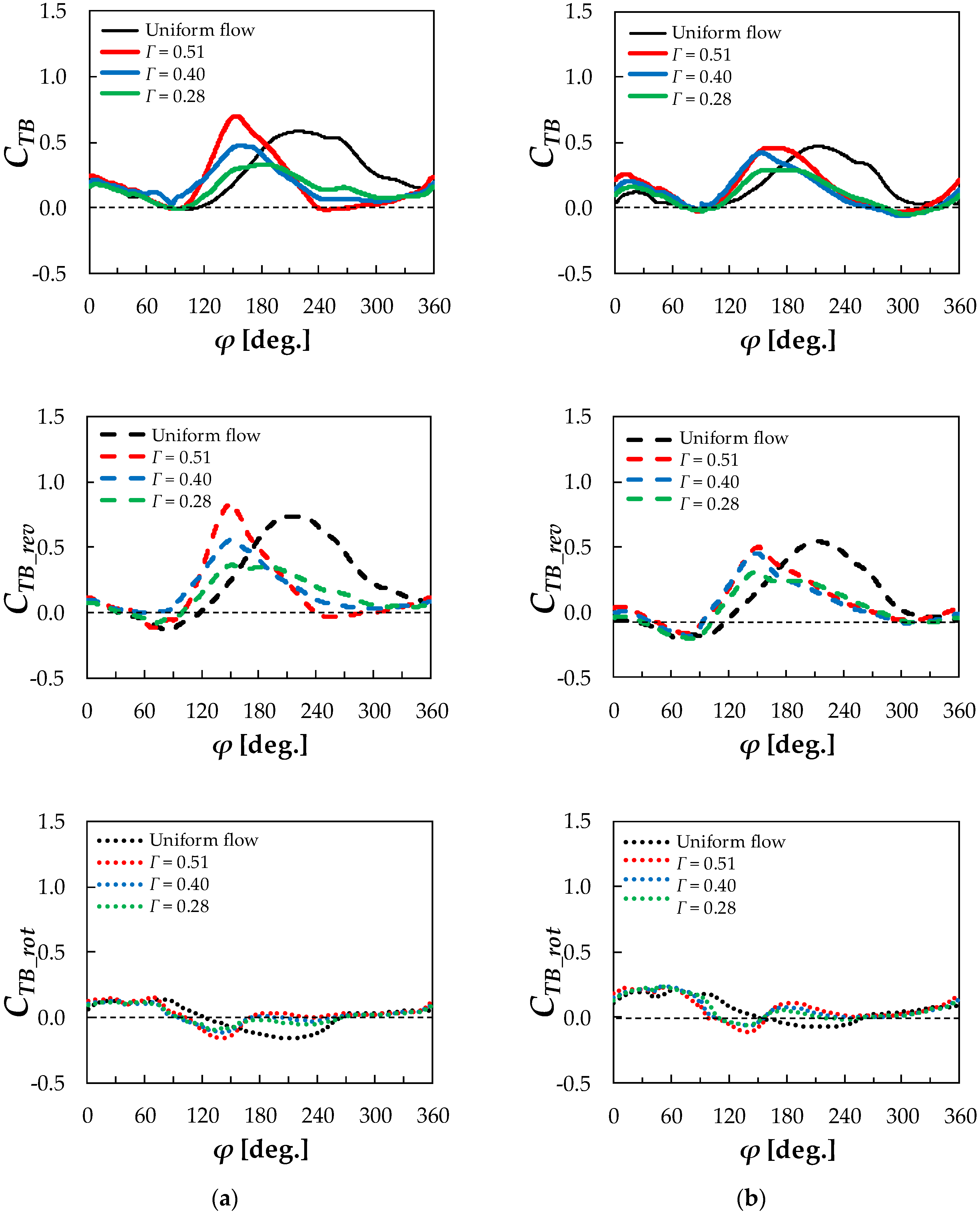
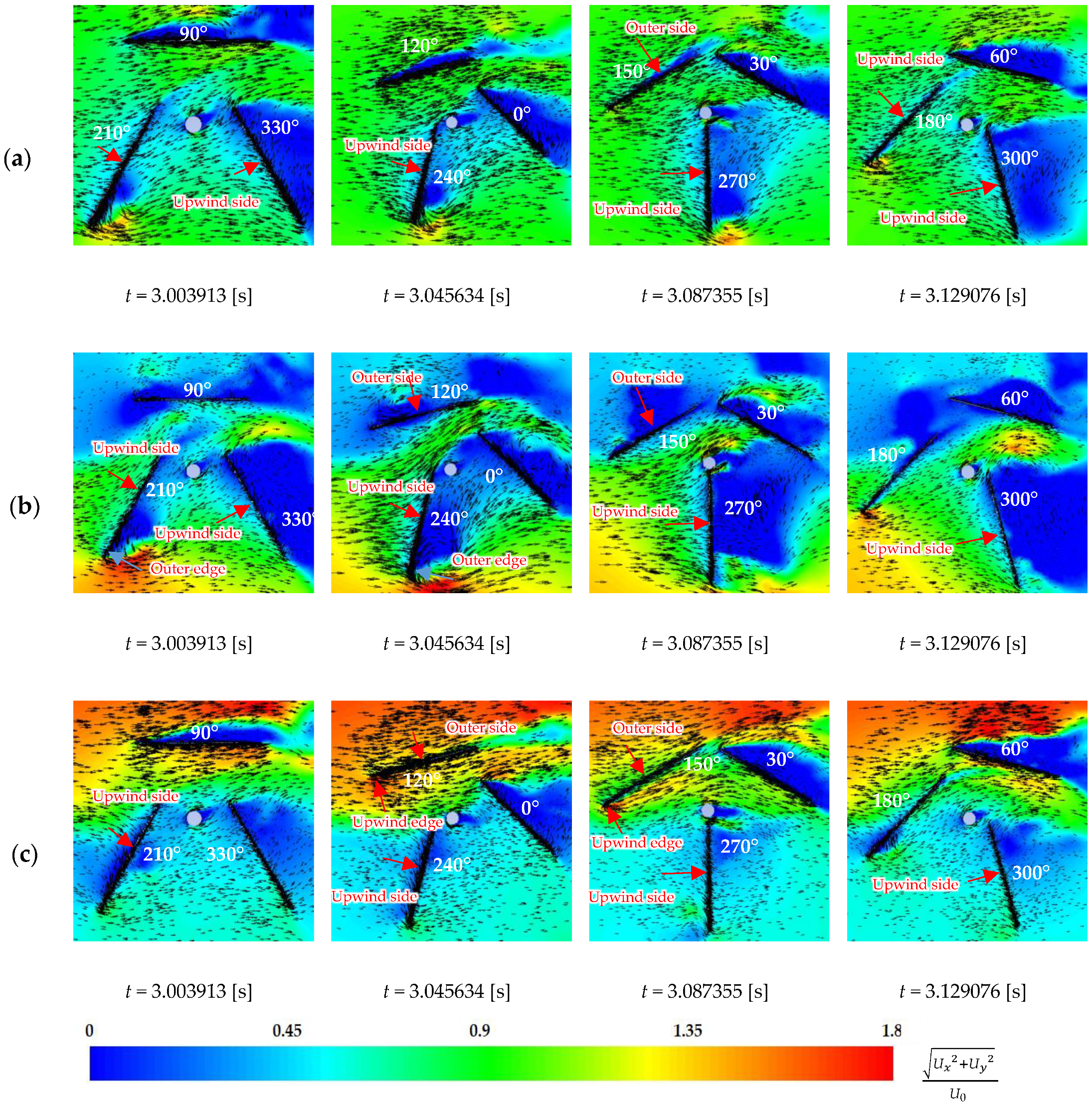
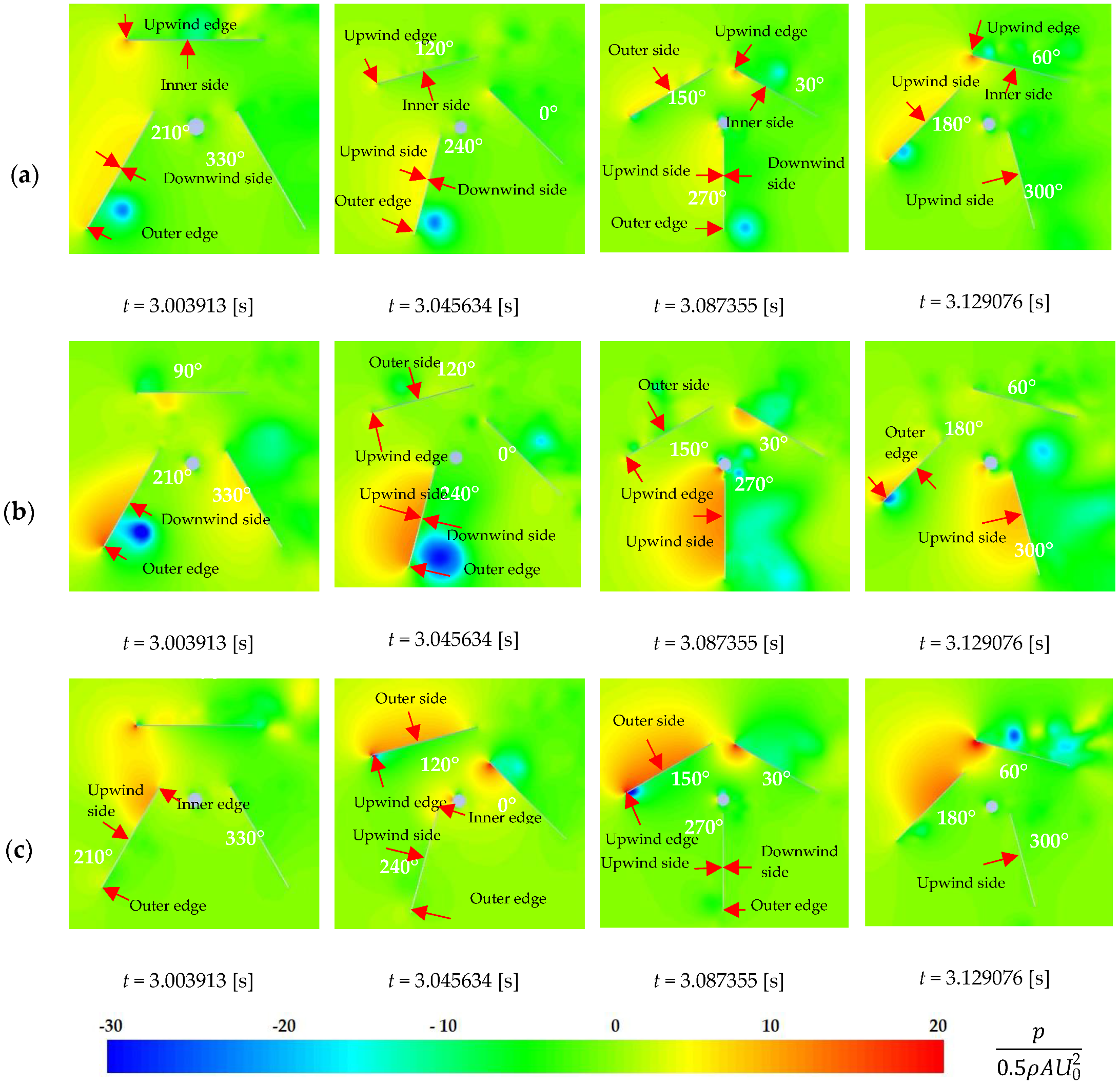
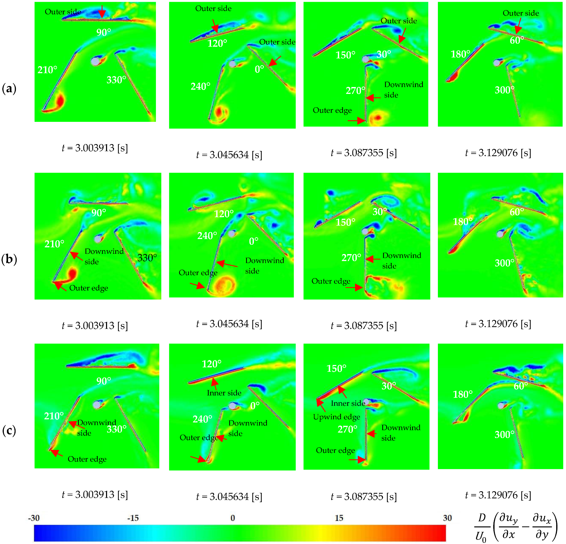
- In the ASF-SF cases, the power coefficients (CP) were significantly higher than the uniform flow case at all tip speed ratios (λ) and increased with Γ. The experimental results for the maximum CP of the ASF-SF case with Γ = 0.51 and the uniform flow case were 0.43 when λ = 0.6 and 0.32 when λ = 0.4, respectively. Around the optimal λ, the blade torque coefficient (CTB) on the advancing side of the rotor was, in general, significantly higher than the uniform flow case and increased with Γ, predominantly contributing to the increase in CP. The CFD results for the maximum discrepancies of CTB on the advancing side of the rotor between the ASF-SF case with Γ = 0.51 and the uniform flow case were 0.38 when λ = 0.4 and 0.44 when λ = 0.6. The high values of CTB of the ASF-SF cases on the advancing side of the rotor were mainly caused by the higher pressure on the upwind side of the blade due to the higher speed of the approaching flow and by the lower pressure near the outer edge of the downwind side of the blade due to the formation of a larger vortex.
- In the RSF-SF cases, CP increased with Γ. However, when Γ = 0.28, CP was lower than the uniform flow case at all λ. When Γ = 0.51, CP was higher than the uniform flow case except at low λ; however, it was lower than the ASF-SF case with Γ = 0.28. The experimental results for the maximum CP of the RSF-SF case with Γ = 0.28, the RSF-SF case with Γ = 0.51 and the ASF-SF case with Γ = 0.28 were 0.29 when λ = 0.4, 0.33 when λ = 0.5 and 0.35 when λ = 0.5, respectively. Around the optimal λ, the blade torque coefficient (CTB) on the retreating side of the rotor was, in general, higher than the uniform flow case and increased with Γ, predominantly contributing to the increase in CP. The CFD results for the maximum discrepancies of CTB on the retreating side of the rotor between the RSF-SF case with Γ = 0.51 and the uniform flow case were 0.60 when λ = 0.4 and 0.36 when λ = 0.6. The high values of CTB of the RSF-SF cases on the retreating side of the rotor were mainly caused by the higher pressure on the outer side of the blade on the upwind side of the rotor, due to the higher speed of the approaching flow. By contrast, CTB on the advancing side of the rotor was, in general, lower than the uniform flow case, due to the lower pressure on the upwind side of the blade.
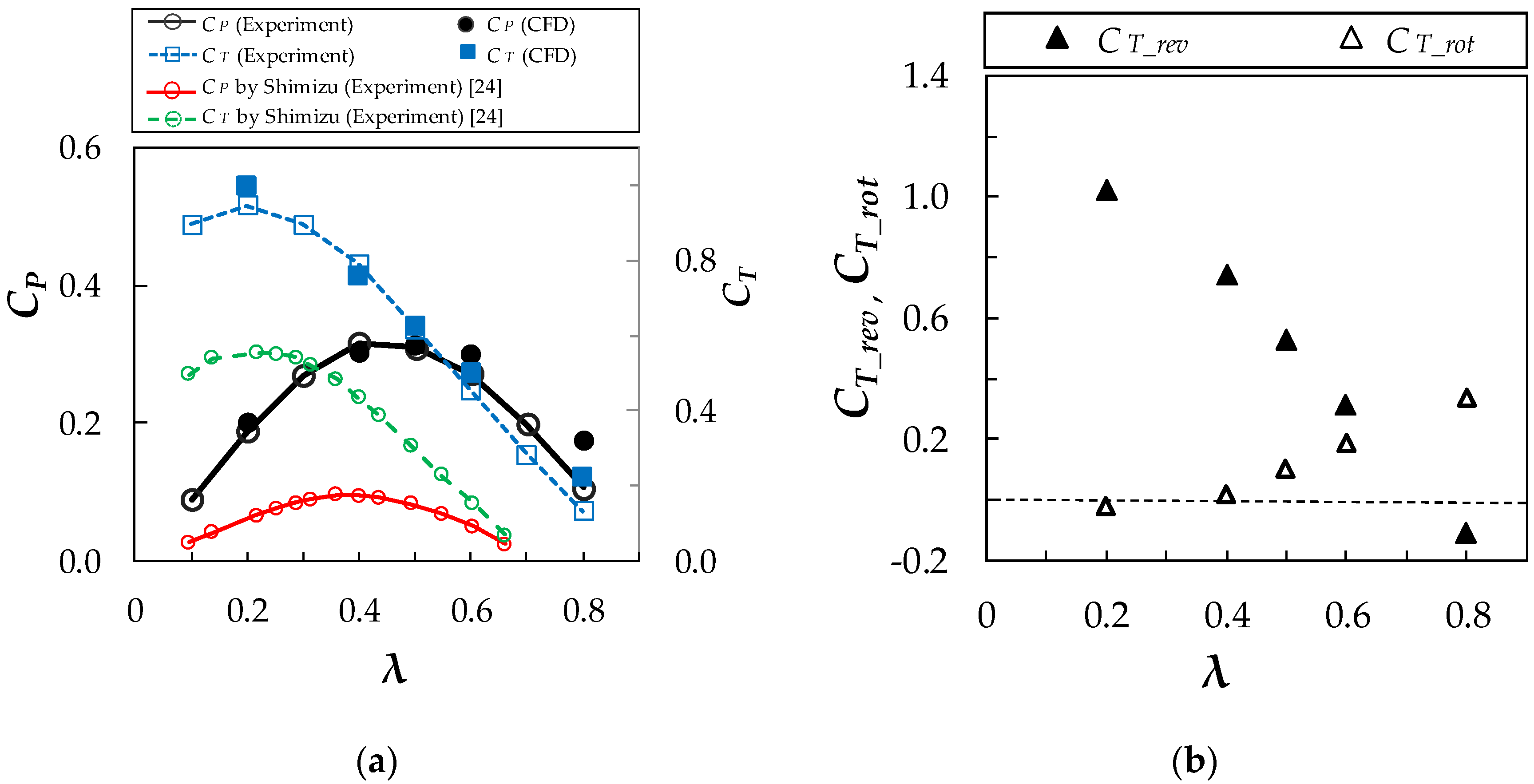
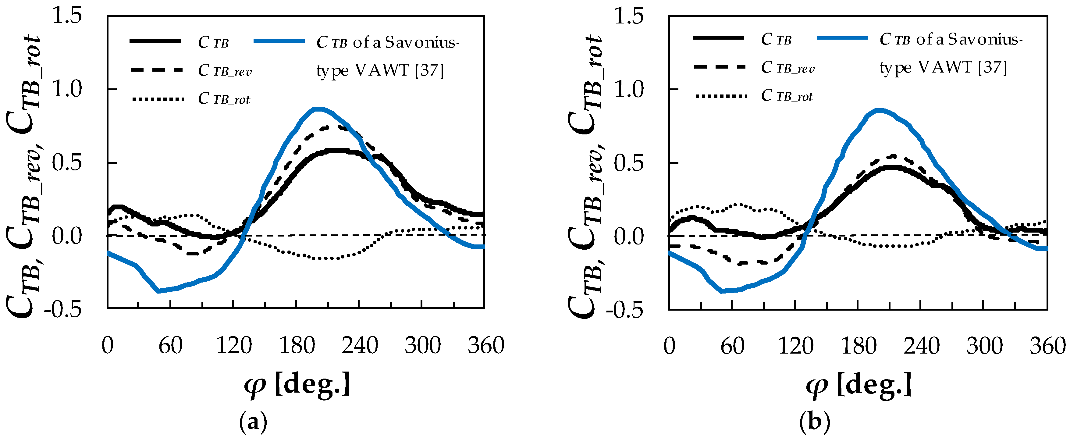
- CTB consists of the rotor-revolution component (CTB_rev) and the blade-rotation component (CTB_rot). In all the shear flow cases, as well as the uniform flow case, the contributions of CTB_rev to CTB were dominant. The dependencies of CTB_rev and CTB_rot on Γ had the opposite tendencies.
Author Contributions
Funding
Acknowledgments
Conflicts of Interest
References
- Bahaj, A.S.; Myers, L.; James, P.A.B. Urban energy generation: Influence of micro-wind turbine output on electricity consumption in buildings. Energy Build. 2007, 39, 154–165. [Google Scholar] [CrossRef]
- Toja-Silva, F.; Colmenar-Santos, A.; Castro-Gil, M. Urban wind energy exploitation systems: Behaviour under multidirectional flow conditions—Opportunities and challenges. Renew. Sustain. Energy Rev. 2013, 24, 364–378. [Google Scholar] [CrossRef]
- Ishugah, T.F.; Li, Y.; Wang, R.Z.; Kiplagat, J.K. Advances in wind energy resource exploitation in urban environment: A review. Renew. Sustain. Energy Rev. 2014, 37, 613–626. [Google Scholar] [CrossRef]
- Tummala, A.; Velamati, R.K.; Sinha, D.K.; Indraja, V.; Krishna, V.H. A review on small scale wind turbines. Renew. Sustain. Energy Rev. 2016, 56, 1351–1371. [Google Scholar] [CrossRef]
- Kumar, R.; Raahemifar, K.; Fung, A.S. A critical review of vertical axis wind turbines for urban applications. Renew. Sustain. Energy Rev. 2018, 89, 281–291. [Google Scholar] [CrossRef]
- Stathopoulos, T.; Alrawashdeh, H.; Al-Quraan, A.; Blocken, B.; Dilimulati, A.; Paraschivoiu, M.; Pilay, P. Urban wind energy: Some views on potential and challenges. J. Wind Eng. Ind. Aerodyn. 2018, 179, 146–157. [Google Scholar] [CrossRef]
- Toja-Silva, F.; Kono, T.; Peralta, C.; Lopez-Garcia, O.; Chen, J. A review of computational fluid dynamics (CFD) simulations of the wind flow around buildings for urban wind energy exploitation. J. Wind Eng. Ind. Aerodyn. 2018, 180, 66–87. [Google Scholar] [CrossRef]
- Anup, K.C.; Whale, J.; Urmee, T. Urban wind conditions and small wind turbines in the built environment: A review. Renew. Energy 2019, 131, 268–283. [Google Scholar]
- Carbó Molina, A.; De Troyer, T.; Massai, T.; Vergaerde, A.; Runacres, M.C.; Bartoli, G. Effect of turbulence on the performance of VAWTs: An experimental study in two different wind tunnels. J. Wind Eng. Ind. Aerodyn. 2019, 193, 103969. [Google Scholar] [CrossRef]
- Wood, D. Small Wind Turbines; Green Energy and Technology; Springer: London, UK, 2011; ISBN 978-1-84996-174-5. [Google Scholar]
- Manwell, J.F.; McGowan, J.G.; Rogers, A.L. Wind Energy Explained: Theory, Design and Application; John Wiley & Sons: Hoboken, NJ, USA, 2010; ISBN 9780470015001. [Google Scholar]
- Allen, S.R.; Hammond, G.P.; McManus, M.C. Prospects for and barriers to domestic micro-generation: A United Kingdom perspective. Appl. Energy 2008, 85, 528–544. [Google Scholar] [CrossRef]
- Islam, M.; Ting, D.S.K.; Fartaj, A. Aerodynamic models for Darrieus-type straight-bladed vertical axis wind turbines. Renew. Sustain. Energy Rev. 2008, 12, 1087–1109. [Google Scholar] [CrossRef]
- Jin, X.; Zhao, G.; Gao, K.; Ju, W. Darrieus vertical axis wind turbine: Basic research methods. Renew. Sustain. Energy Rev. 2015, 42, 212–225. [Google Scholar] [CrossRef]
- Ghasemian, M.; Ashrafi, Z.N.; Sedaghat, A. A review on computational fluid dynamic simulation techniques for Darrieus vertical axis wind turbines. Energy Convers. Manag. 2017, 149, 87–100. [Google Scholar] [CrossRef]
- Kumar, P.M.; Sivalingam, K.; Narasimalu, S.; Lim, T.-C.; Ramakrishna, S.; Wei, H. A review on the evolution of darrieus vertical axis wind turbine: Small wind turbines. J. Power Energy Eng. 2019, 7, 27–44. [Google Scholar] [CrossRef]
- Abraham, J.P.; Plourde, B.D.; Mowry, G.S.; Minkowycz, W.J.; Sparrow, E.M. Summary of Savonius wind turbine development and future applications for small-scale power generation. J. Renew. Sustain. Energy 2012, 4, 042703. [Google Scholar] [CrossRef]
- Akwa, J.V.; Vielmo, H.A.; Petry, A.P. A review on the performance of Savonius wind turbines. Renew. Sustain. Energy Rev. 2012, 16, 3054–3064. [Google Scholar] [CrossRef]
- Roy, S.; Saha, U.K. Review on the numerical investigations into the design and development of Savonius wind rotors. Renew. Sustain. Energy Rev. 2013, 24, 73–83. [Google Scholar] [CrossRef]
- Kang, C.; Liu, H.; Yang, X. Review of fluid dynamics aspects of Savonius-rotor-based vertical-axis wind rotors. Renew. Sustain. Energy Rev. 2014, 33, 499–508. [Google Scholar] [CrossRef]
- Alom, N.; Saha, U.K. Evolution and progress in the development of savonius wind turbine rotor blade profiles and shapes. J. Sol. Energy Eng. Trans. ASME 2019, 141, 1–15. [Google Scholar] [CrossRef]
- Elkhoury, M.; Kiwata, T.; Nagao, K.; Kono, T.; ElHajj, F. Wind tunnel experiments and Delayed Detached Eddy Simulation of a three-bladed micro vertical axis wind turbine. Renew. Energy 2018, 129, 63–74. [Google Scholar] [CrossRef]
- Kiwata, T. Vertical axis wind turbine with variable-pitch straight blades. In Proceedings of the International Conferemce on Jets, Wakes and Separated Flows, ICJWSF-2017, Cincinnati, OH, USA, 9–12 October 2017; pp. 1–6. [Google Scholar]
- Shimizu, Y.; Maeda, T.; Kamada, Y.; Takada, M.; Katayama, T. Development of micro wind turbine (Orthoptere Wind Turbine). In Proceedings of the International Conference on Fluid Engineering JSME Centennial Grand Congress, Tokyo, Japan, 13–16 July 1997; pp. 1551–1556. [Google Scholar]
- Bayeul-Laine, A.-C.; Simonet, S.; Dockter, A.; Bois, G. Numerical study of flow stream in a mini VAWT with relative rotating blades. In Proceedings of the 22nd International Symposium on Transport Phenomena Conference, Delft, The Netherlands, 8–11 November 2011; p. 13. [Google Scholar]
- Cooper, P.; Kennedy, O.C.; Cooper, P.; Kennedy, O. Development and analysis of a novel vertical axis wind turbine development and analysis of a novel vertical axis wind turbine. In Proceedings of the Solar 2004: Life, The Universe and Renewables, Perth, Australia, 30 November–3 December 2004; pp. 1–9. [Google Scholar]
- Kono, T.; Kogaki, T.; Kiwata, T. Numerical investigation ofwind conditions for roof-mounted wind turbines: Effects of wind direction and horizontal aspect ratio of a high-rise cuboid building. Energies 2016, 9, 907. [Google Scholar] [CrossRef]
- Balduzzi, F.; Bianchini, A.; Ferrari, L. Microeolic turbines in the built environment: Influence of the installation site on the potential energy yield. Renew. Energy 2012, 45, 163–174. [Google Scholar] [CrossRef]
- Ferreira, C.J.S.; Van Bussel, G.J.W.; Van Kuik, G.A.M. Wind tunnel hotwire measurements, flow visualization and thrust measurement of a VAWT in skew. J. Sol. Energy Eng. Trans. ASME 2006, 128, 487–497. [Google Scholar] [CrossRef]
- Burton, T.; Jenkins, N.; Sharpe, D.; Bossanyi, E. Wind Energy Handbook, 2nd ed.; John Wiley & Sons: Hoboken, NJ, USA, 2011; ISBN 9780470699751. [Google Scholar]
- ANSYS, Inc. ANSYS Fluent Theory Guide, Release 17.2; ANSYS, Inc.: Canonsburg, PA, USA, 2016. [Google Scholar]
- ANSYS, Inc. ANSYS Fluent User Guide, Release 17.2; ANSYS, Inc.: Canonsburg, PA, USA, 2016. [Google Scholar]
- ElCheikh, A.; Elkhoury, M.; Kiwata, T.; Kono, T. Performance analysis of a small-scale orthopter-type vertical axis wind turbine. J. Wind Eng. Ind. Aerodyn. 2018, 180, 19–33. [Google Scholar] [CrossRef]
- Spalart, P.R.; Jou, W.H.; Strelets, M.; Allmaras, S.R. Comments on the feasibility of LES for wings, and on a hybrid RANS/LES approach. In Proceedings of the First AFOSR International Conference on DNS/LES, Ruston, LA, USA, 4–8 August 1997; pp. 137–147. [Google Scholar]
- Tominaga, Y.; Mochida, A.; Yoshie, R.; Kataoka, H.; Nozu, T.; Yoshikawa, M.; Shirasawa, T. AIJ guidelines for practical applications of CFD to pedestrian wind environment around buildings. J. Wind Eng. Ind. Aerodyn. 2008, 96, 1749–1761. [Google Scholar] [CrossRef]
- Wu, H.; Stathopoulos, T. Wind-tunnel techniques for assessment of pedestrian-level winds. J. Eng. Mech. 1993, 119, 1920–1936. [Google Scholar] [CrossRef]
- Tian, W.; Mao, Z.; Zhang, B.; Li, Y. Shape optimization of a Savonius wind rotor with different convex and concave sides. Renew. Energy 2018, 117, 287–299. [Google Scholar] [CrossRef]


| Name | d [m] | L [m] | Φ [-] | Enlarged View |
|---|---|---|---|---|
| Perforated panel A | 3 × 10⁻³ | 4 × 10⁻³ | 0.49 |  |
| Perforated panel B | 3 × 10⁻³ | 4.5 × 10⁻³ | 0.60 |  |
| Perforated panel C | 3 × 10⁻³ | 5 × 10⁻³ | 0.67 |  |
| Domain | Mesh on This Research | Regular Mesh Used by ElCheikh [33] |
|---|---|---|
| Blade 1 | 2,300,530 | 1,610,660 |
| Blade 2 | 2,303,725 | 1,614,903 |
| Blade 3 | 2,304,607 | 1,588,363 |
| Blade 4 | - | 1,614,661 |
| Rotor | 1,756,635 | 2,127,497 |
| Far end | 1,770,583 | 441,196 |
| TOTAL | 10,436,080 | 8,997,280 |
| Flow Type | Γ | Φ | UH [m/s] | Range of UH Region [m] | Velocity Distribution in Transition Region | Range of Transition Region [m] | UL [m/s] | Range of UL Region [m] |
|---|---|---|---|---|---|---|---|---|
| Uniform | 0 | - | 8 | 8 | 8 | |||
| ASF-SF | 0.51 | 0.67 | 13.2 | y ≤ −0.24 | UH ∙(−y/0.24)0.3 | −0.24 ≤ y ≤ −0.01 | 4.3 | y ≥ −0.01 |
| ASF-SF | 0.40 | 0.60 | 12.1 | y ≤ −0.22 | UH ∙(−y/0.22)0.35 | −0.22 ≤ y ≤ 0.02 | 5.2 | y ≥ −0.02 |
| ASF-SF | 0.28 | 0.49 | 10.8 | y ≤ −0.18 | UH ∙(−y/0.18)0.2 | −0.18 ≤ y ≤ −0.01 | 6.1 | y ≥ −0.01 |
| RSF-SF | 0.51 | 0.67 | 13.2 | y ≥ 0.24 | UH ∙(y/0.24)0.3 | 0.01 ≤ y ≤ 0.24 | 4.3 | y ≤ 0.01 |
| RSF-SF | 0.40 | 0.60 | 12.1 | y ≥ 0.22 | UH ∙(y/0.24)0.35 | 0.02 ≤ y ≤ 0.22 | 5.2 | y ≤ 0.02 |
| RSF-SF | 0.28 | 0.49 | 10.8 | y ≥ 0.18 | UH ∙(y/0.24)0.2 | 0.01 ≤ y ≤ 0.18 | 6.1 | y ≤ 0.01 |
| Flow Type | Γ | U0 [m/s] | Re | ||
|---|---|---|---|---|---|
| Experiment | CFD | Experiment | CFD | ||
| Uniform | 0 | 8 | 8 | 2.79 × 10⁵ | 2.79 × 10⁵ |
| ASF-SF | 0.51 | 10.08 | 9.78 | 3.52 × 10⁵ | 3.41 × 10⁵ |
| ASF-SF | 0.40 | 9.38 | 9.22 | 3.28 × 10⁵ | 3.22 × 10⁵ |
| ASF-SF | 0.28 | 8.73 | 8.72 | 3.05 × 10⁵ | 3.05 × 10⁵ |
| RSF-SF | 0.51 | 7.76 | 7.48 | 2.71 × 10⁵ | 2.61 × 10⁵ |
| RSF-SF | 0.40 | 7.72 | 7.36 | 2.70 × 10⁵ | 2.57 × 10⁵ |
| RSF-SF | 0.28 | 7.52 | 7.33 | 2.62 × 10⁵ | 2.56 × 10⁵ |
© 2020 by the authors. Licensee MDPI, Basel, Switzerland. This article is an open access article distributed under the terms and conditions of the Creative Commons Attribution (CC BY) license (http://creativecommons.org/licenses/by/4.0/).
Share and Cite
Wijayanto, R.P.; Kono, T.; Kiwata, T. Performance Characteristics of an Orthopter-Type Vertical Axis Wind Turbine in Shear Flows. Appl. Sci. 2020, 10, 1778. https://doi.org/10.3390/app10051778
Wijayanto RP, Kono T, Kiwata T. Performance Characteristics of an Orthopter-Type Vertical Axis Wind Turbine in Shear Flows. Applied Sciences. 2020; 10(5):1778. https://doi.org/10.3390/app10051778
Chicago/Turabian StyleWijayanto, Rudi Purwo, Takaaki Kono, and Takahiro Kiwata. 2020. "Performance Characteristics of an Orthopter-Type Vertical Axis Wind Turbine in Shear Flows" Applied Sciences 10, no. 5: 1778. https://doi.org/10.3390/app10051778
APA StyleWijayanto, R. P., Kono, T., & Kiwata, T. (2020). Performance Characteristics of an Orthopter-Type Vertical Axis Wind Turbine in Shear Flows. Applied Sciences, 10(5), 1778. https://doi.org/10.3390/app10051778