Evaluation of Tip Loss Corrections to AD/NS Simulations of Wind Turbine Aerodynamic Performance

Abstract

The Actuator Disc/Navier-Stokes (AD/NS) method has played a significant role in wind farm simulations. It is based on the assumption that the flow is azimuthally uniform in the rotor plane, and thus, requires a tip loss correction to take into account the effect of a finite number of blades. All existing tip loss corrections were originally proposed for the Blade-Element Momentum Theory (BEMT), and their implementations have to be changed when transplanted into the AD/NS method. The special focus of the present study is to investigate the performance of tip loss corrections combined in the AD/NS method. The study is conducted by using an axisymmetric AD/NS solver to simulate the flow past the experimental NREL Phase Ⅵ wind turbine and the virtual NREL 5MW wind turbine. Three different implementations of the widely used Glauert tip loss function F are discussed and evaluated. In addition, a newly developed tip loss correction is applied and compared with the above implementations. For both the small and large rotors under investigation, the three different implementations show a certain degree of difference to each other, although the relative difference in blade loads is generally no more than 4%. Their performance is roughly consistent with the standard Glauert correction employed in the BEMT, but they all tend to make the blade tip loads over-predicted. As an alternative method, the new tip loss correction shows superior performance in various flow conditions. A further investigation into the flow around and behind the rotors indicates that tip loss correction has a significant influence on the velocity development in the wake.

1. Introduction

Wind energy is nowadays an important and increasing source of electric power. It has been the biggest contributor of renewable electricity except for hydropower, sharing about 5.5% of the global electricity production in 2018 [1]. As a primary subject of wind turbine technology, aerodynamics [2] largely determines the efficiency of wind energy extraction of an individual wind turbine or a wind farm. Along with the extensive development of high quality wind resources onshore, there are several trends in wind power industry: A large number of newly installed wind turbines have to be installed in areas with lower wind speeds and complex terrain; the layout optimization of wind turbine array becomes very important for wind farm design; offshore wind power development is accelerating, and the rotor size is continuously increasing. These trends need to be supported by more advanced and refined aerodynamic tools. More accurate aerodynamic load prediction is required for the design of a new generation of wind turbines with high efficiency and relatively low weight. Furthermore, a wind farm with dozens of wind turbines needs to be studied as a whole in order to take into account the complex interference between wind turbines.

Blade Element Momentum Theory (BEMT) [3,4] and Computational Fluid Dynamics (CFD) [5,6] are two essential methods of wind turbine aerodynamic computation. BEMT is no doubt the key method for rotor design [7], while CFD gives the most refined data of aerodynamic loads and flow parameters. A full CFD simulation with resolved rotor geometry is usually employed for an individual wind turbine [8,9]. However, full CFD is not suitable for a wind turbine array, due to the huge computational cost. The Actuator Disc/Navier-Stokes (AD/NS) method [10,11,12,13] was developed for this situation, in which the rotor geometry is not resolved, and thus, the number of mesh cells is greatly reduced. AD/NS is based on a combination of the blade-element theory and CFD. The flow field is still solved by CFD, while the rotor entity is replaced by a virtual actuator disc on which an external body force is acted. If the blade entities are represented by virtual actuator lines, it is called the Actuator Lines/Navier-Stokes (AL/NS) method [14,15,16,17]. As compared to AD/NS, the flow around the rotor solved by AL/NS is closer to the reality, since the rotor vortices are simulated. However, AL/NS requires more grid cells to describe the actuator lines, and thus, is seldom employed in wind farm simulations.

The AD/NS method has played a significant role in wind farm simulations involving wake interaction [18,19], complex terrain [20,21], atmospheric boundary layer [22,23], noise propagation [24,25], etc. Nevertheless, the AD model assumes that the number of blades is infinite, and thus, no tip loss is simulated, causing an over-prediction of the blade tip loads and power output. In order to take tip loss into account, a reliable engineering model has to be embedded into the numerical solver, which is usually called tip loss correction. However, all tip loss corrections were originally proposed for BEMT, and there is no tip loss correction specially developed for AD/NS. Most of the literature about AD/NS simulations either did not mention tip loss or declared that the Glauert tip loss correction [26] was employed. It is worth mentioning that AD/NS and BEMT solve the momentum of the flow past the rotor by using two completely different approaches. The former employs CFD, while the latter applies the momentum theory, though they share the actuator disc assumption and the blade-element theory. That leads to different implementations of tip loss correction for the two methods. In the BEMT, tip loss correction is realized by applying a correction factor F into the induced velocity through the rotor. In the AD/NS, the velocity is naturally found by the NS solver, and factor F can only be used to modify the external body force. The question is whether a tip loss correction has a good global performance when it is transplanted into AD/NS. Even for the BEMT itself, evaluations indicate that accurate tip loss correction is still not well achieved [27], and the development of new correction models is still going on [28,29,30,31,32,33]. In contrast with the massive study in the BEMT, tip loss corrections applied to AD/NS lack a comprehensive evaluation.

In the present work, the 2-Dimensional (2D) axisymmetric AD model is employed, and steady-state simulations are performed. The code solves the incompressible axisymmetric NS equations for the experimental NREL Phase Ⅵ wind turbine [34] and the virtual NREL 5MW [35] wind turbine under various axial inflow conditions. The main purpose of the numerical study is to evaluate the performance of the tip loss corrections applied to AD/NS. Three different implementations of the Glauert tip loss correction are discussed. In addition, a new tip loss correction recently proposed by Zhong et al. [33] is introduced and compared. The normal and tangential forces of blade cross-sections are chosen as the key parameters for the present evaluation. Because of the long arm of force, computational errors of the forces acted on the tip region are most likely to cause non-ignorable errors of the blade bending moment and the rotor torque (power generation). A BEMT study on the NREL Phase Ⅵ wind turbine by Branlard [27] showed that the power generation would be overestimated by 15% if no tip loss correction was made and a deviation of about 5% exists when various existing tip loss corrections were applied. That highlights the significance of the present study on tip loss correction.

The innovation of the present study lies in the following items. (a) Different implementations of the Glauert tip loss factor F are gathered, discussed and compared, and finally, one of them is recommended according to its best performance. Such kind of work has never been reported in the existing literature. (b) The Glauert correction is found to have a similar performance when it is transplanted from BEMT to AD/NS. (c) The new tip loss correction of Zhong et al. [33] is for the first time employed in AD/NS simulations. It is found to be generally superior to the Glauert-type corrections. That provides an alternative choice for a more accurate prediction of the blade tip loads. (d) Tip loss correction is found to have a significant influence on the velocity field, which highlights the importance of an accurate tip loss correction for not only the blade loads, but also the wake development.

The paper is organized as follows: In Section 2, the axisymmetric AD/NS method is introduced, including the governing equations of the NS approach and the formulae of the AD model; In Section 3, the Glauert and the new tip loss corrections are introduced; In Section 4, the implementations of the tip loss corrections used in AD/NS are described; In Section 5, the numerical setup, as well as the involved simulation cases, are introduced; In Section 6, all simulation results are presented and discussed; Final conclusions are made in the last section.

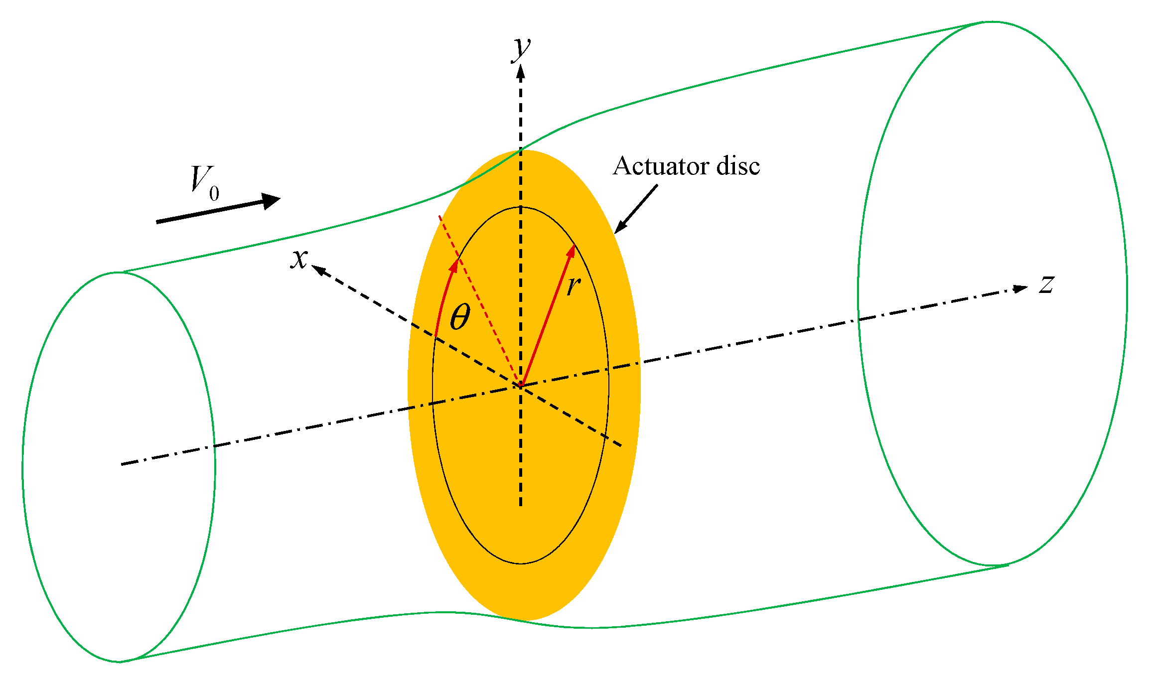
2. Axisymmetric AD/NS Method

2.1. Governing Equations

The governing equations of the present AD/NS simulation are the incompressible axisymmetric NS equations. In a cylindrical coordinate system as shown in Figure 1, the axial direction is defined along the z-axis, the radial direction is represented by r, and the tangential direction is represented by $\theta$, the continuity equation is written as

$$\nabla \cdot \overrightarrow{u}=\frac{\partial u_z}{\partial z}+\frac{\partial u_r}{\partial r}+\frac{u_r}{r}=0,$$

(1)

the axial and radial momentum equations read

$$\frac{\partial u_z}{\partial t}+\frac{1}{r}\frac{\partial }{\partial z}(r{u}_z^2)+\frac{1}{r}\frac{\partial }{\partial r}(r{u}_r{u}_z)=-\frac{1}{\rho }\frac{\partial p}{\partial z}+\frac{1}{r}\frac{\partial }{\partial z}\left[r\nu \left(2\frac{\partial u_z}{\partial z}-\frac{2}{3}\left(\nabla \cdot \overrightarrow{u}\right)\right)\right]+\frac{1}{r}\frac{\partial }{\partial r}\left[r\nu \left(\frac{\partial u_z}{\partial r}+\frac{\partial u_r}{\partial z}\right)\right]+f_z,$$

(2)

$$\begin{array}{l}\frac{\partial u_r}{\partial t}+\frac{1}{r}\frac{\partial }{\partial z}(r{u}_z{u}_r)+\frac{1}{r}\frac{\partial }{\partial r}(r{u}_r^2)=\\ -\frac{1}{\rho }\frac{\partial p}{\partial r}+\frac{1}{r}\frac{\partial }{\partial z}\left[r\nu \left(\frac{\partial u_r}{\partial z}+\frac{\partial u_z}{\partial r}\right)\right]+\frac{1}{r}\frac{\partial }{\partial r}\left[r\nu \left(2\frac{\partial u_r}{\partial r}-\frac{2}{3}\left(\nabla \cdot \overrightarrow{u}\right)\right)\right]-2\nu \frac{u_r}{r^2}+\frac{2}{3}\frac{\nu }{r}\left(\nabla \cdot \overrightarrow{u}\right)+\frac{u_{\theta }^2}{r}+f_r\end{array}$$

(3)

and the tangential momentum equation is

$$\frac{\partial u_{\theta }}{\partial t}+\frac{1}{r}\frac{\partial }{\partial z}(r{u}_z{u}_{\theta })+\frac{1}{r}\frac{\partial }{\partial r}(r{u}_r{u}_{\theta })=\frac{1}{r}\frac{\partial }{\partial z}\left(r\nu \frac{\partial u_{\theta }}{\partial z}\right)+\frac{1}{r^2}\frac{\partial }{\partial r}\left[r^3\nu \frac{\partial }{\partial r}\left(\frac{u_{\theta }}{r}\right)\right]-\frac{u_r{u}_{\theta }}{r}+f_{\theta }.$$

(4)

In the above equations, $u_z$/$u_r$/$u_{\theta }$ is the axial/radial/tangential velocity, $p$ is the static pressure, $\rho$ is the air density, $\nu$ is the kinematic viscosity coefficient of air, $f_z$, $f_r$, $f_{\theta }$ are the source term of the axial, radial, tangential external body forces, respectively.

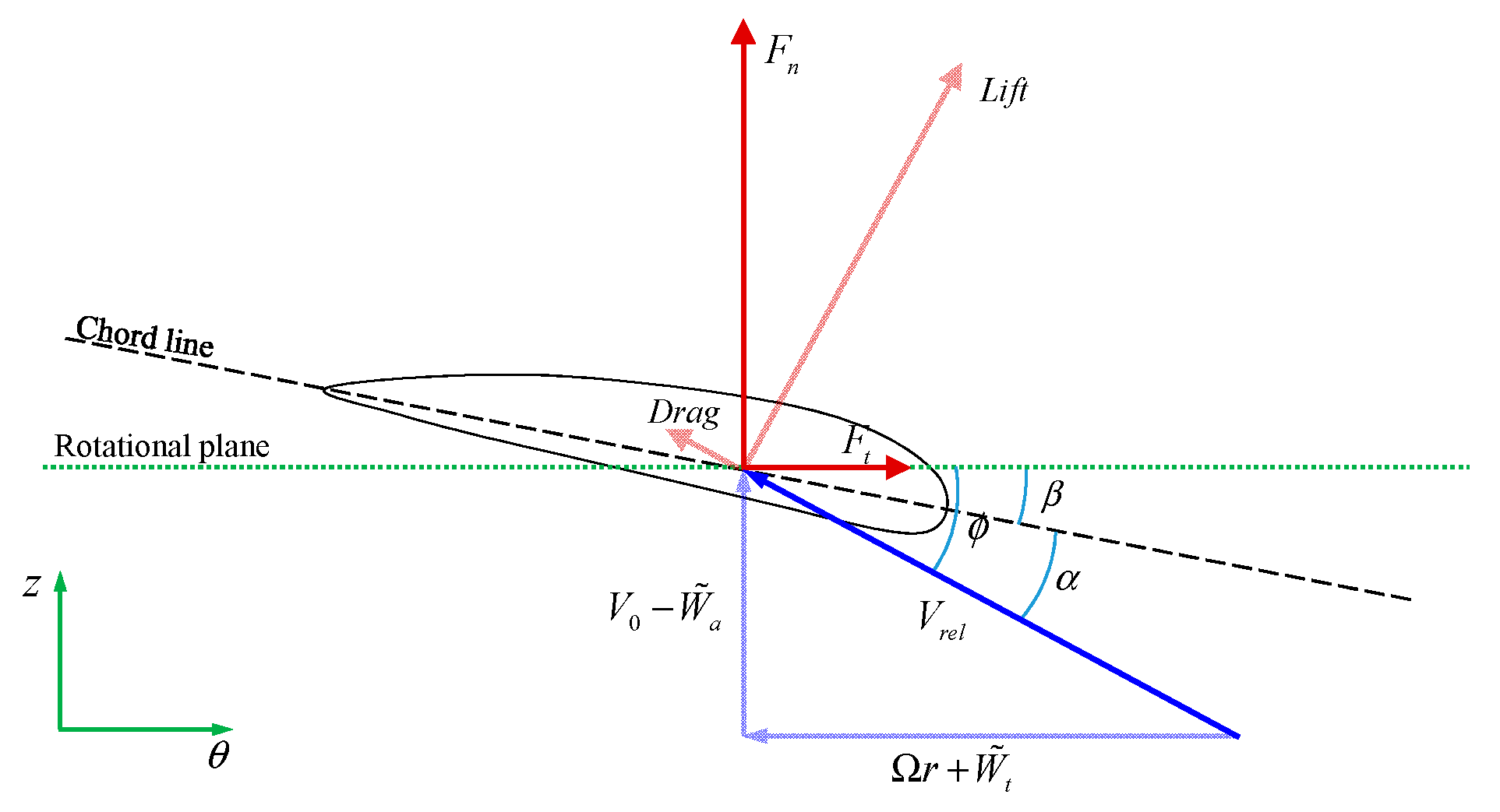
2.2. Force on Actuator Disc

The conceptual idea of the AD/NS method is to solve the aerodynamic force of rotor blades by using the blade-element theory and then applying its counterforce as an external body force into the momentum equations.

At each time step of solving the NS equations, the velocity passing through the actuator disc is detected and used to determine the axial induced velocity $W_a$ and the tangential induced velocity $W_t$,

$$W_a=V_0-u_z,$$

(5)

$$W_t=-u_{\theta }.$$

(6)

The axial interference factor $a$ and tangential interference factor $a^{\prime }$ are then determined by,

$$a=\frac{W_a}{V_0},$$

(7)

$$a^{\prime }=\frac{W_t}{\mathsf{\Omega }r},$$

(8)

where $V_0$ is the wind speed, and $\mathsf{\Omega }$ is the rotating speed of the wind turbine rotor.

The above interference factors are azimuthally unchanged according to the axisymmetric condition, which implies an infinite number of blades and zero tip loss. In order to estimate the tip loss of the realistic rotor with a finite number of blades, the interference factors need to be corrected as

$$\tilde{a}=f_{corr}(a),$$

(9)

$${\tilde{a}}^{\prime }={f^{\prime }}_{corr}(a^{\prime }),$$

(10)

where $\tilde{a}$ and ${\tilde{a}}^{\prime }$ denote the corrected axial and tangential interference factors, $f_{corr}$ and $f_{corr}^{\prime }$ represent correction functions.

The axial and tangential induced velocities after the correction are written as

$${\tilde{W}}_a=V_0\tilde{a},$$

(11)

$${\tilde{W}}_t=\mathsf{\Omega }r\widetilde{a^{\prime }}.$$

(12)

According to the velocity triangle shown in Figure 2, the flow angle $\varphi$, angle of attack $\alpha$, and relative velocity $V_{rel}$ are then determined by

$$\varphi ={\tan }^{-1}\left(\frac{V_0-{\tilde{W}}_a}{\mathsf{\Omega }r+{\tilde{W}}_t}\right),$$

(13)

$$\alpha =\varphi -\beta ,$$

(14)

$$V_{rel}^2={\left(V_0-{\tilde{W}}_a\right)}^2+{\left(\mathsf{\Omega }r+{\tilde{W}}_t\right)}^2,$$

(15)

where $\beta$ is the local pitch angle of a blade cross-section.

With the determined angle of attack and relative velocity, the lift coefficient $C_l$ and drag coefficient $C_d$ of each cross-section of the blade can be obtained from tabulated airfoil data. According to the relationship of force projection, the normal and tangential force coefficients are determined by

$$C_n=C_l\cos \varphi +C_d\sin \varphi ,$$

(16)

$$C_t=C_l\sin \varphi -C_d\cos \varphi ,$$

(17)

The axial force $F_z$ and tangential force $F_{\theta }$ per radial length of the rotor are then given by

$$F_z=\frac{1}{2}\rho V_{rel}^{2}cB{C}_n=\frac{1}{2}\rho V_{rel}^{2}cB\left(C_l\cos \varphi +C_d\sin \varphi \right),$$

(18)

$$F_{\theta }=\frac{1}{2}\rho V_{rel}^{2}cB{C}_t=\frac{1}{2}\rho V_{rel}^{2}cB\left(C_l\sin \varphi -C_d\cos \varphi \right),$$

(19)

where $c$ is the local chord length, and $B$ is the number of blades. Ignoring the effect of the radial flow, the vector form of the counterforce acting on the air is

$$\overrightarrow{F}=\left(-F_z,0,-F_{\theta }\right).$$

(20)

Rather than distributing the force only on the disc, the above force is regularized by the following Gaussian distribution along the axial direction in order to avoid a numerical singularity. The Gaussian distribution has been widely used and proven to be proper for AD/NS and AL/NS simulations [10,14,15,16,17].

$${\overrightarrow{F}}_{\epsilon }={\eta }_{\epsilon }\overrightarrow{F},{\eta }_{\epsilon }=\frac{1}{\epsilon \sqrt{\pi }}\exp \left[-{\left(\frac{z-z_0}{\epsilon }\right)}^2\right],$$

(21)

where $z_0$ is the axial position of the disc. The parameter $\epsilon$ serves to adjust the concentration of the regularized force, which is in the present study set to $\epsilon$ = 0.02R where R is the rotor radius.

The source terms of the external body force in the momentum Equations (2)–(4) need to be replaced with the above force per unit volume. In the axisymmetric coordinate system, a 2D grid cell with an axial length of $\mathsf{\Delta }z$ and a radial height of $\mathsf{\Delta }r$ represents a volume of $2\pi r\mathsf{\Delta }r\mathsf{\Delta }z$, and thus, the force per unit volume is

$$\overrightarrow{f}=\frac{{\overrightarrow{F}}_{\epsilon }\mathsf{\Delta }r\mathsf{\Delta }z}{2\pi r\mathsf{\Delta }r\mathsf{\Delta }z}=\frac{{\overrightarrow{F}}_{\epsilon }}{2\pi r},$$

(22)

Using Equations (20) and (21), it reads

$$\overrightarrow{f}=\frac{{\eta }_{\epsilon }\overrightarrow{F}}{2\pi r}=\left(-\frac{{\eta }_{\epsilon }{F}_z}{2\pi r},0,-\frac{{\eta }_{\epsilon }{F}_{\theta }}{2\pi r}\right),$$

(23)

i.e.,

$$\{\begin{array}{c}{f}_z=-\frac{{\eta }_{\epsilon }{F}_z}{2\pi r}\\ f_r=0\\ f_{\theta }=-\frac{{\eta }_{\epsilon }{F}_{\theta }}{2\pi r}\end{array}.$$

(24)

3. Tip Loss Corrections

3.1. Glauert Correction

The tip loss correction of Glauert [26] was developed from the study of Prandtl [36]. A function F, which was later recognized as the first tip loss factor, was derived by Prandtl making Betz’s optimal circulation [37] go to zero at the blade tip,

$$F=\frac{2}{\pi }\arccos \left\{\exp \left[-\frac{B}{2}\left(1-\frac{r}{R}\right)\sqrt{1+{\lambda }^2}\right]\right\},$$

(25)

where B is the number of blades, r is the local radial location, R is the rotor radius, and λ is the tip speed ratio. The original derivation of Prandtl was written very briefly and was elaborated more in [4,27,38] as for a more detailed derivation.

Later on, Glauert made further contributions. First, he interpreted the physical meaning of factor F as the ratio between the azimuthally averaged induced velocity and the induced velocity at the blade position, leading to

$$F=\frac{\overline{a}}{a_B}=\frac{\overline{a^{\prime }}}{a_B^{\prime }},$$

(26)

where $\overline{a}=\frac{1}{2\pi }{\int }_0^{2\pi }a\mathrm{d}\theta$ and ${\overline{a}}^{\prime }=\frac{1}{2\pi }{\int }_0^{2\pi }{a}^{\prime }\mathrm{d}\theta$ are the azimuthally averaged axial and tangential interference factors, and $a_B$ and $a_B^{\prime }$ are the interference factors at the blade position. Second, the local inflow angle $\varphi$ was introduced into the function in order to make it consistent with the local treatment of the BEMT, leading to the following new formula of factor F,

$$F=\frac{2}{\pi }\arccos \left\{\exp \left[-\frac{B\left(R-r\right)}{2r\sin \varphi }\right]\right\}.$$

(27)

The factor F was then applied into the momentum theory through a straightforward way of multiplying the axial velocity at the rotor plane with factor F, resulting in the following thrust and torque for an annular element,

$$\mathrm{d}T=4\pi r\rho V_0^{2}a\left(1-a\right)F\mathrm{d}r,$$

(28)

$$\mathrm{d}M=4\pi r^3\rho V_0\mathsf{\Omega }{a}^{\prime }\left(1-a\right)F\mathrm{d}r.$$

(29)

Using another two equations of $\mathrm{d}T$ and $\mathrm{d}M$ derived from the blade-element theory,

$$\mathrm{d}T=\frac{1}{2}\rho V_{rel}^{2}c{C}_{n}B\mathrm{d}r=\frac{1}{2}\rho V_{rel}^{2}c\left(C_l\cos \varphi +C_d\sin \varphi \right)B\mathrm{d}r,$$

(30)

$$\mathrm{d}M=\frac{1}{2}\rho V_{rel}^{2}c{C}_{t}Br\mathrm{d}r=\frac{1}{2}\rho V_{rel}^{2}c\left(C_l\sin \varphi -C_d\cos \varphi \right)Br\mathrm{d}r,$$

(31)

and the velocity triangle at the rotor plane, the equations for the interference factors in the BEMT approach was derived to be:

$$\frac{a}{1-a}=\frac{\sigma \left(C_l\cos \varphi +C_d\sin \varphi \right)}{4F{\sin }^2\varphi },$$

(32)

$$\frac{a^{\prime }}{1+a^{\prime }}=\frac{\sigma \left(C_l\sin \varphi -C_d\cos \varphi \right)}{4F\sin \varphi \cos \varphi }.$$

(33)

The above two equations lead to the final iterative formulae of the BEMT approach with the Glauert tip loss correction. Their difference from the baseline BEMT approach is only the appearance of factor F in the equations. Obviously, the application of the Glauert correction in BEMT is very simple, which is also a great advantage. There are several variations of the Glauert correction in which the way of applying factor F is different [39,40], but the original Glauert tip loss correction is the most commonly used form till today.

3.2. A Newly Developed Correction

A new tip loss correction was recently proposed for BEMT by Zhong et al. [33], based on a novel insight into tip loss. In contrast with the Prandtl/Glauert series corrections that begin with an actuator disc and estimate the effect of the finite number of blades, the new correction begins with a non-rotating blade and estimates the effect of rotation on tip loss. It has been validated in BEMT computations and showed superior performances in the cases involving flow separation or high axial interference factor.

The correction was realized by using two factors of $F_R$ and $F_S$ that treat the rotational effect and the 3D effect, respectively.

$$F_R=2-\frac{2}{\pi }\arccos \left\{\exp \left[-2B\left(1-r/R\right)\sqrt{1+{\lambda }^2}\right]\right\},$$

(34)

$$F_S=\frac{2}{\pi }\arccos \left\{\exp \left[-{\left(\frac{1-r/R}{\overline{c}/R}\right)}^{3/4}\right]\right\},\overline{c}=\frac{S_{\mathrm{t}}}{R-r},$$

(35)

where $\overline{c}$ denotes a geometric mean chord length, and $S_{\mathrm{t}}$ is the projected area of the blade between the present cross-section and the tip. The purpose of introducing $\overline{c}$ is to deal with tapered blades and those with sharp tips.

The factor $F_R$ was applied to the BEMT approach by using:

$$\frac{a{F}_R\left(1-a{F}_R\right)}{\left(1-a\right)}=\frac{\sigma \left({\tilde{C}}_l\cos \varphi +{\tilde{C}}_d\sin \varphi \right)}{4{\sin }^2\varphi },$$

(36)

$$\frac{a^{\prime }{F}_R(1-a{F}_R)}{(1+a^{\prime })(1-a)}=\frac{\sigma \left({\tilde{C}}_l\sin \varphi -{\tilde{C}}_d\cos \varphi \right)}{4\sin \varphi \cos \varphi },$$

(37)

in which the employed lift and drag coefficients were corrected by factor $F_S$, rather than the direct use of the airfoil data.

$${\tilde{C}}_l=\frac{1}{2}\left[C_l(\alpha )F_S+C_l^{*}\right],$$

(38)

$${\tilde{C}}_d=\frac{1}{{\cos }^2{\alpha }_i}\left[C_d({\alpha }_e)\cos {\alpha }_i+\left({\tilde{C}}_l\cos {\alpha }_i+C_d({\alpha }_e)\tan {\alpha }_i\right)\sin {\alpha }_i\right];$$

(39)

where

$$C_l^{*}=\frac{1}{{\cos }^2{\alpha }_i}\left[C_l({\alpha }_e)\cos {\alpha }_i-C_d({\alpha }_e)\sin {\alpha }_i\right],$$

(40)

$${\alpha }_i=\frac{C_l(\alpha )}{m}\left(1-F_S\right),$$

(41)

where m is the slope of the lift-curve of the airfoil before flow separation, ${\alpha }_i$ is called the downwash angle, and ${\alpha }_e$ is called the effective angle of attack.

By comparing with the Glauert tip loss correction, the new tip loss correction appears more complicated in application. It is simplified in the present study: First, Equations (36) and (37) will not be employed naturally in the AD/NS method; Second, Equations (38)–(41) are further simplified to

$${\tilde{C}}_l=\frac{1}{2}\left[C_l(\alpha )F_S+C_l({\alpha }_e)\right],{\alpha }_e=\alpha -{\alpha }_i,$$

(42)

$${\tilde{C}}_d=C_d({\alpha }_e)+{\tilde{C}}_l\tan {\alpha }_i,{\alpha }_i=\frac{C_l(\alpha )}{m}\left(1-F_S\right).$$

(43)

The simplification is derived by using the fact that ${\alpha }_i$ and $C_d$ are relatively small. More detailed applications are shown in the next section.

4. Applying Corrections to AD/NS Simulation

4.1. Application of Glauert Tip Loss Factor F

Equations (32) and (33) where the Glauert tip loss factor F is applied are not employed in the AD/NS method because the flow is simulated by the NS solver instead of the momentum theory. As a result, an alternative way has to be employed correctly to apply the tip loss factor F. Nevertheless, among the literature studies, little literature mentions the detail of how the tip loss factor is applied to the AD/NS simulations. After an extensive literature review, we have found three representative documents in which Sørensen et al. [41], Mikkelsen [42], and Shen et al. [43] described their implementations. In order to facilitate the distinction, the implementations adopted by the three studies are denoted as Glauert-A, Glauert-B and Glauert-C in the present paper, respectively.

4.1.1. Glauert-A Correction

Sørensen et al. [41] performed a tip loss correction by applying factor F to modify the aerodynamic force that determines the external body force in the NS equations. They replaced the lift coefficient $C_l$ by $C_l/F$ (there was no need to modify the drag in their study as the drag was assumed not to produce the external body force). In the present Glauert-A correction, $C_n$ and $C_t$, in Equations (18) and (19), are replaced by:

$${\tilde{C}}_n=C_n/F,$$

(44)

$${\tilde{C}}_t=C_t/F.$$

(45)

That is equivalent to replacing $C_l$ by $C_l/F$ and $C_d$ by $C_d/F$, according to Equations (16) and (17).

Sørensen et al. [41] did not explain the reason why factor F could be directly used to modify the force. They might be inspired by Equations (32) and (33) in which the existence of F can be looked as corrections to $C_n$ and $C_t$, although from a physical point of view it is a correction to the interference factors. It is important to note that the corrected force is only used for determining the external body force, so as the flowfield, while the force acting on the blade should be regarded as the original one. In addition, the interference factors in Equations (9) and (10) should no longer be corrected, leading to $\tilde{a}=a$ and ${\tilde{a}}^{\prime }=a^{\prime }$.

This implementation involves a division operation with denominator F, which causes unreasonable big values of ${\tilde{C}}_n$ and ${\tilde{C}}_t$ at the extreme tip where $F\to 0$. However, there is no exact criterion for defining what a big value is unreasonable because the ${\tilde{C}}_n$ and ${\tilde{C}}_t$ themselves are introduced as an engineering correction rather than a physical concept. Sørensen et al. [41] did not mention this problem, and no obvious numerical fluctuation is observed in his result. That is possible because the problem is limited to a very small area at the tip, and thus, the integral effect of the resulted unreasonable body force is also small.

4.1.2. Glauert-B Correction

Mikkelsen [42] compared Equations (32) and (33) to the corresponding baseline equations without factor F. The baseline equations are

$$\frac{a}{1-a}=\frac{\sigma \left(C_l\cos \varphi +C_d\sin \varphi \right)}{4{\sin }^2\varphi },$$

(46)

$$\frac{a^{\prime }}{1+a^{\prime }}=\frac{\sigma \left(C_l\sin \varphi -C_d\cos \varphi \right)}{4\sin \varphi \cos \varphi }.$$

(47)

In order to distinguish from the parameters in the baseline equations, we here rewrite equations (32) and (33) to

$$\frac{F\tilde{a}}{\left(1-\tilde{a}\right)}=\frac{\sigma \left({\tilde{C}}_l\cos \tilde{\varphi }+{\tilde{C}}_d\sin \tilde{\varphi }\right)}{4{\sin }^2\tilde{\varphi }},$$

(48)

$$\frac{F{\tilde{a}}^{\prime }}{\left(1+{\tilde{a}}^{\prime }\right)}=\frac{\sigma \left({\tilde{C}}_l\sin \tilde{\varphi }-{\tilde{C}}_d\cos \tilde{\varphi }\right)}{4\sin \tilde{\varphi }\cos \tilde{\varphi }}.$$

(49)

The implementation of Mikkelsen [42] adopts the following equations which implies an assumption of $\varphi =\tilde{\varphi }$ which in fact does not accurately hold,

$$\frac{a}{1-a}=\frac{\sigma \left(C_l\cos \varphi +C_d\sin \varphi \right)}{4{\sin }^2\varphi }=\frac{F\tilde{a}}{\left(1-\tilde{a}\right)},$$

(50)

$$\frac{a^{\prime }}{1+a^{\prime }}=\frac{\sigma \left(C_l\sin \varphi -C_d\cos \varphi \right)}{4\sin \varphi \cos \varphi }=\frac{F{\tilde{a}}^{\prime }}{\left(1+{\tilde{a}}^{\prime }\right)}.$$

(51)

The corrected interference factors were, thus, determined by

$$\tilde{a}=\frac{a}{F(1-a)+a},$$

(52)

$${\tilde{a}}^{\prime }=\frac{a^{\prime }}{F(1+a^{\prime })-a^{\prime }}.$$

(53)

The tip loss correction was completed as the above functions for $\tilde{a}$ and ${\tilde{a}}^{\prime }$ were used to replace Equations (9) and (10).

4.1.3. Glauert-C Correction

Shen et al. [43] performed their correction by directly using Equation (26) which represents the physical meaning of factor F. Using the azimuthally uniform condition ($\overline{a}$ = $a$), the correction was completed by replacing Equations (9) and (10) with

$$\tilde{a}=a_B=a/F,$$

(54)

$${\tilde{a}}^{\prime }=a_B^{\prime }=a^{\prime }/F.$$

(55)

Similar to the Glauert-A correction, this implementation involves a division operation with denominator F. That causes an unphysical big value of $\tilde{a}$ at the extreme tip where $F\to 0$. A limiter is set in the present study to force the result to be $\tilde{a}$ = 1 when it is greater than 1. The value of ${\tilde{a}}^{\prime }$ is usually much less than $\tilde{a}$ and is not limited here.

4.2. Application of New Correction

The application of the new correction consists of two steps: The first is using factor $F_R$ determined by Equation (34) and the second is using factor $F_S$ determined by Equation (35).

In the first step, an implementation similar to the Glauert-C correction is adopted, which is performed by replacing Equations (9) and (10) with

$$\tilde{a}=a/F_R,$$

(56)

$${\tilde{a}}^{\prime }=a^{\prime }/F_R.$$

(57)

A limiter of $\tilde{a}$ = 1 is used when $\tilde{a}$ is greater than 1. The angle of attack $\alpha$ can then be determined by calculations using Equations (11)–(14).

The second step is to correct the lift and drag coefficients by using Equations (42) and (43), the result of which is used to replace the $C_l$ and $C_d$ in Equations (18) and (19).

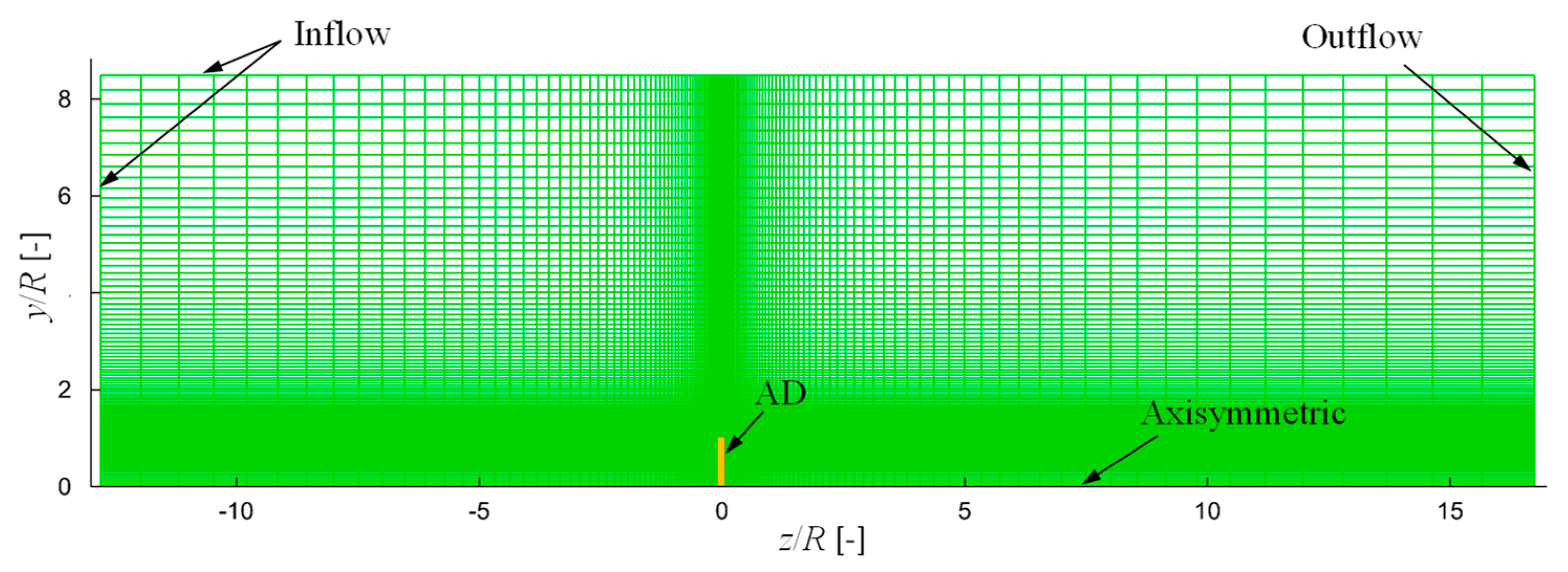
5. Computational Setup

5.1. Flow Solver and Mesh Configuration

The 2D axisymmetric NS equations are solved by using an in-house code EllipSys2D [44,45] developed at Technical University of Denmark (DTU). The code is a general incompressible flow solver with multi-block and multi-grid strategy. The equations are discretized with a second-order finite volume method. In the spatial discretization, a central difference scheme is applied to the diffusive terms and the QUICK (Quadratic Upstream Interpolation for Convective Kinematics) upwind scheme is applied to the convective terms. The SIMPLEC (Semi-Implicit Method for Pressure-Linked Equations) scheme is used for the velocity-pressure decoupling. The turbulence flow is simulated using the method of Reynolds-averaged Navier-Stokes equations (RANS) in which the k-ω turbulence model of Menter [46] is employed with a modification for a better simulation of the turbulence quantities in the free-stream flow [47,48].

The coordinate for the AD/NS simulations is defined in the z-y plane. A computational mesh is generated, as shown in Figure 3 where the inflow, outflow and axisymmetric boundaries are indicated, the length of the computational domain is 30, which is nondimensionalized with the rotor radius. The blade is positioned at z = 0 and the grid cells are clustered around z = 0 and y = 1 to ensure a better resolution near the blade tip. The mesh is composed of four blocks where 64 × 64 grid points are used for each block. There are 64 grid points on the AD along the radial direction, and 20 points in the range of [-0.02, 0.02] in the axial direction where the Gaussian distribution of the body force plays a significant role. Since the axisymmetric boundary condition is applied, the 2D flow solution is regarded as an azimuthal slice of a full 3D field.

The above computational setup has been proven to perform well in AD/NS simulations, as shown in the previous work of Cao et al. [49] where both blade loads and wake flows were validated against experiments.

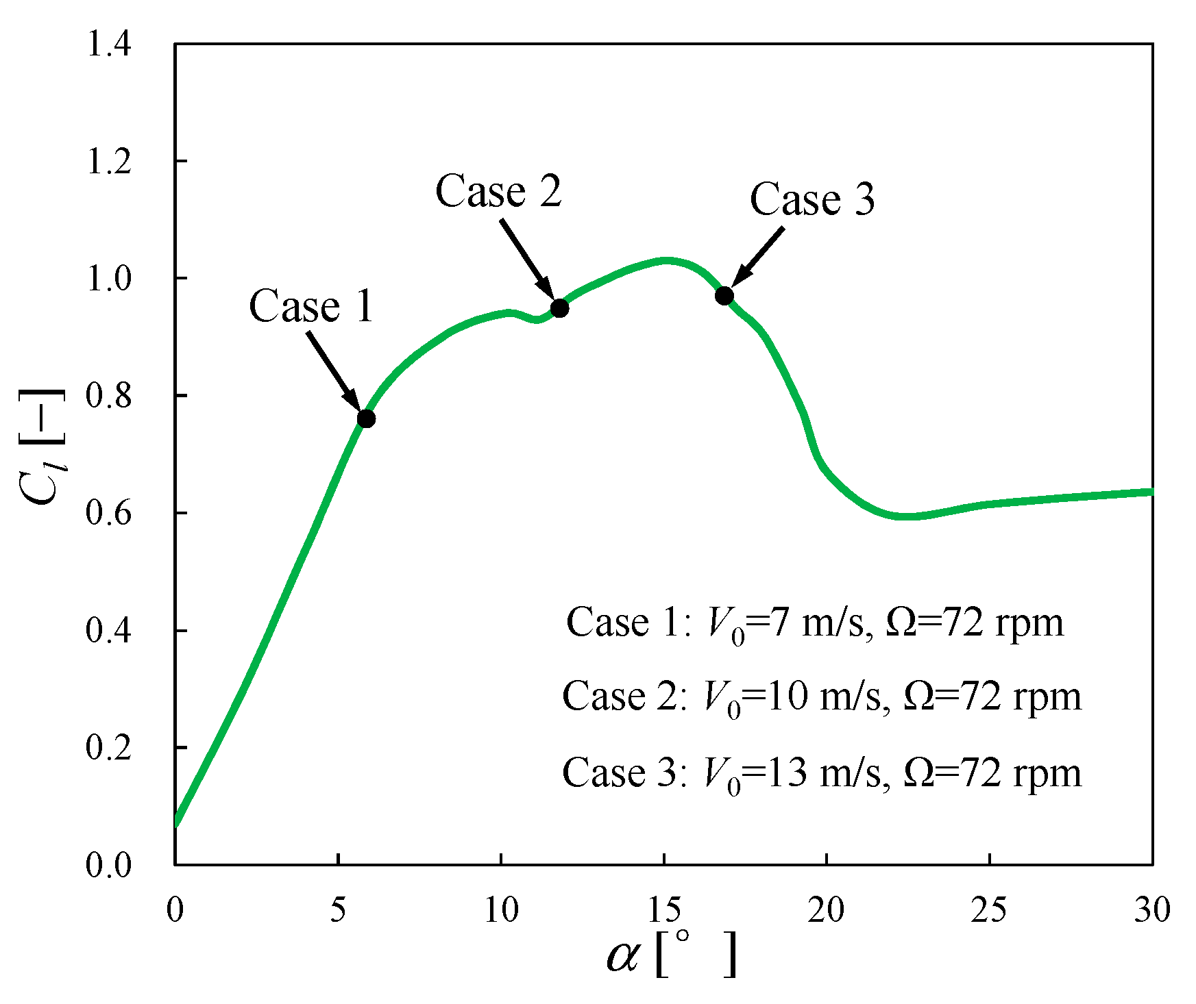
5.2. Simulation Cases

Simulations are performed for two different wind turbines of the NREL Phase Ⅵ [34] and the NREL 5MW [35] that represent a small and a large rotor size, respectively. Additionally, the NREL Phase Ⅵ rotor has a very blunt blade tip shape as compared with the NREL 5MW rotor.

The operational conditions of the two rotors are listed in

Table 1. Simulation cases for two different wind turbines.

Rotor Name	Number	Wind Speed (V0, m/s)	Rotating Speed (Ω, rpm)	Tip Speed Ratio (λ)	Tip Pitch Angle (°)
NREL PhaseⅥ	1	7.0	72	5.4	3
	2	10.0	72	3.8	3
	3	13.0	72	2.9	3
NREL 5MW	4	8.0	9.22	7.60	0
	5	11.4	12.06	6.98	0

. Cases 1, 2 and 3 are set to be consistent with the NREL UAE experiment in axial inflow conditions [34]. Various wind speeds of 7 m/s, 10 m/s and 13 m/s are considered, while the rotating speed remains unchanged. The flow is fully attached on the blade surface at a wind speed of 7 m/s, but is partly separated at 10 m/s and 13 m/s (Higher wind speed leads to heavier flow separation) [8]. Measured pressure distributions (from which the force can be obtained by pressure integral) at five blade sections (r/R = 0.30, 0.47, 0.63, 0.80, 0.95) are available for these cases [50]. Cases 4 and 5 are two typical points on the designed power curve of the NREL 5MW wind turbine [35]. The wind speed and rotating speed of Case 5 are the rated parameters of this wind turbine. Case 4 represents a condition with a lower wind speed of 8 m/s at which the rotating speed is reduced to 9.22 rpm for tracking the optimum tip speed ratio.

These cases cover the following multiple situations: Wind turbines with remarkably different rotor sizes and tip shapes; flow with fully attached and separated conditions; operating conditions with various wind speeds and rotating speeds. It is, therefore, interesting to see the performance of the tip loss corrections in these cases.

Experimental data are preferred as the reference for the computational results of the NREL Phase Ⅵ rotor, as well as the full CFD data are also displayed in some results. For the cases of the NREL 5MW rotor, there is no experimental data available such that the full CFD data are the only reference. The related full CFD simulations were previously conducted by the authors, see Zhong et al. [8,33].

6. Simulation Results

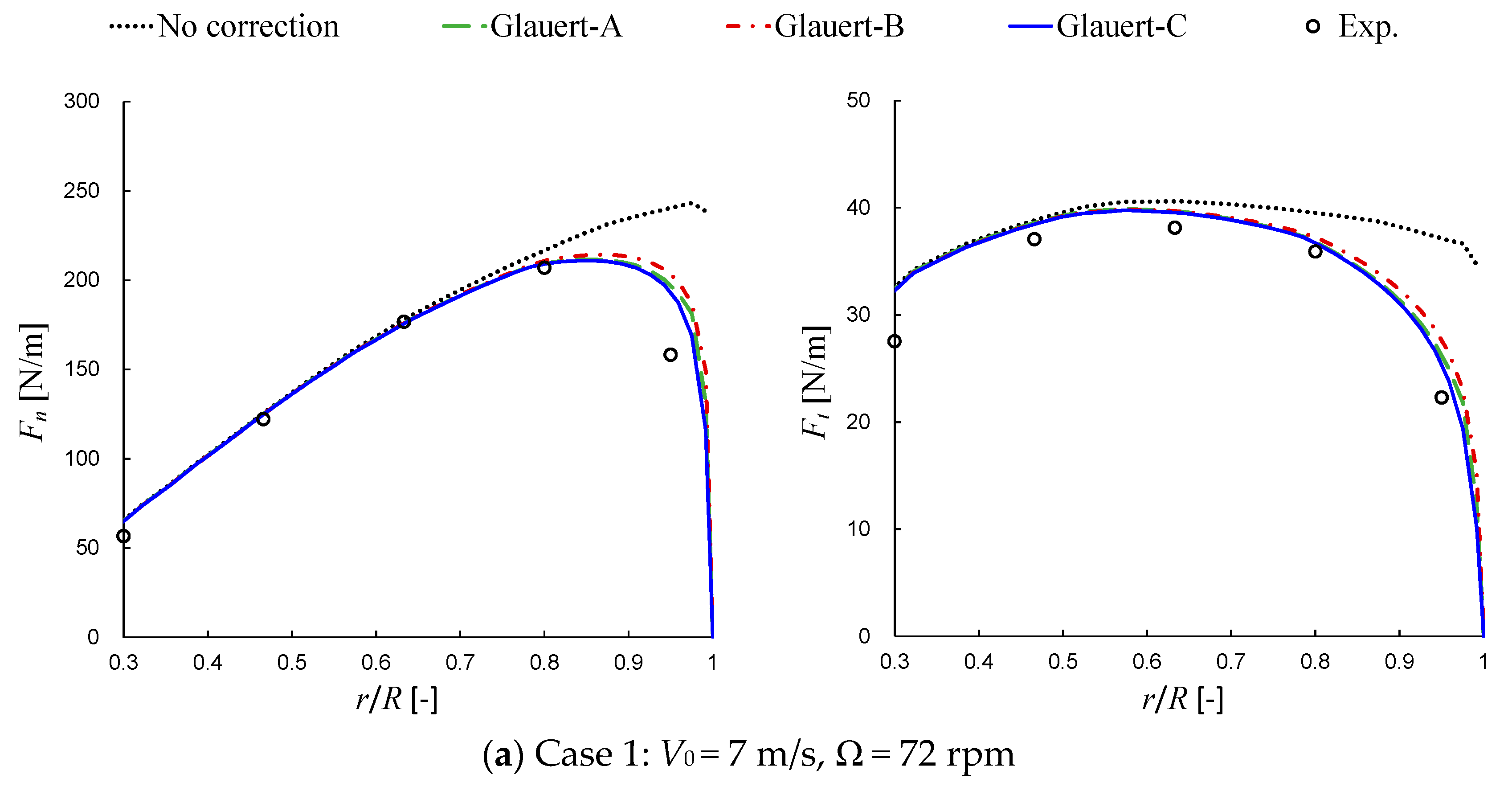
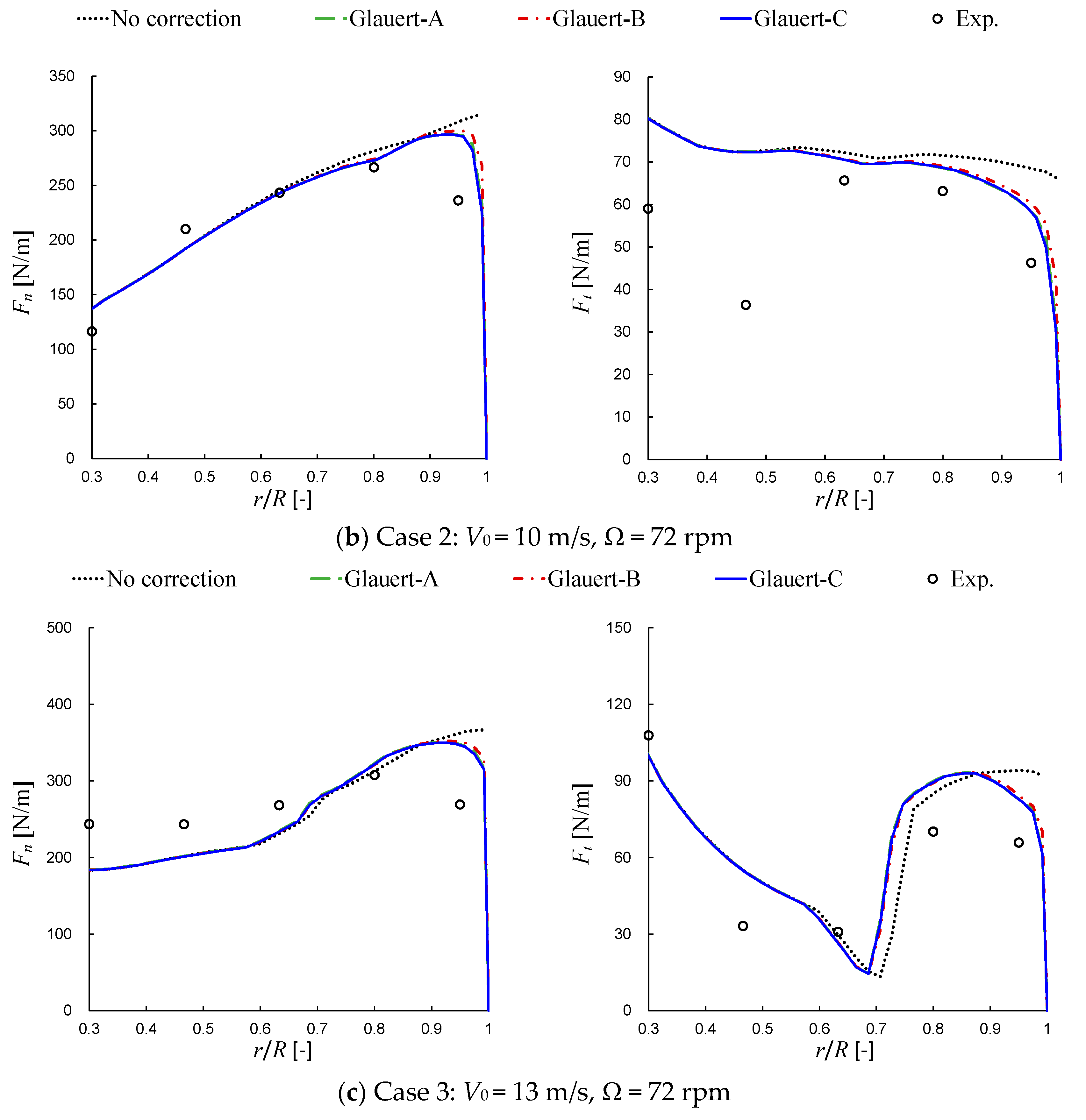
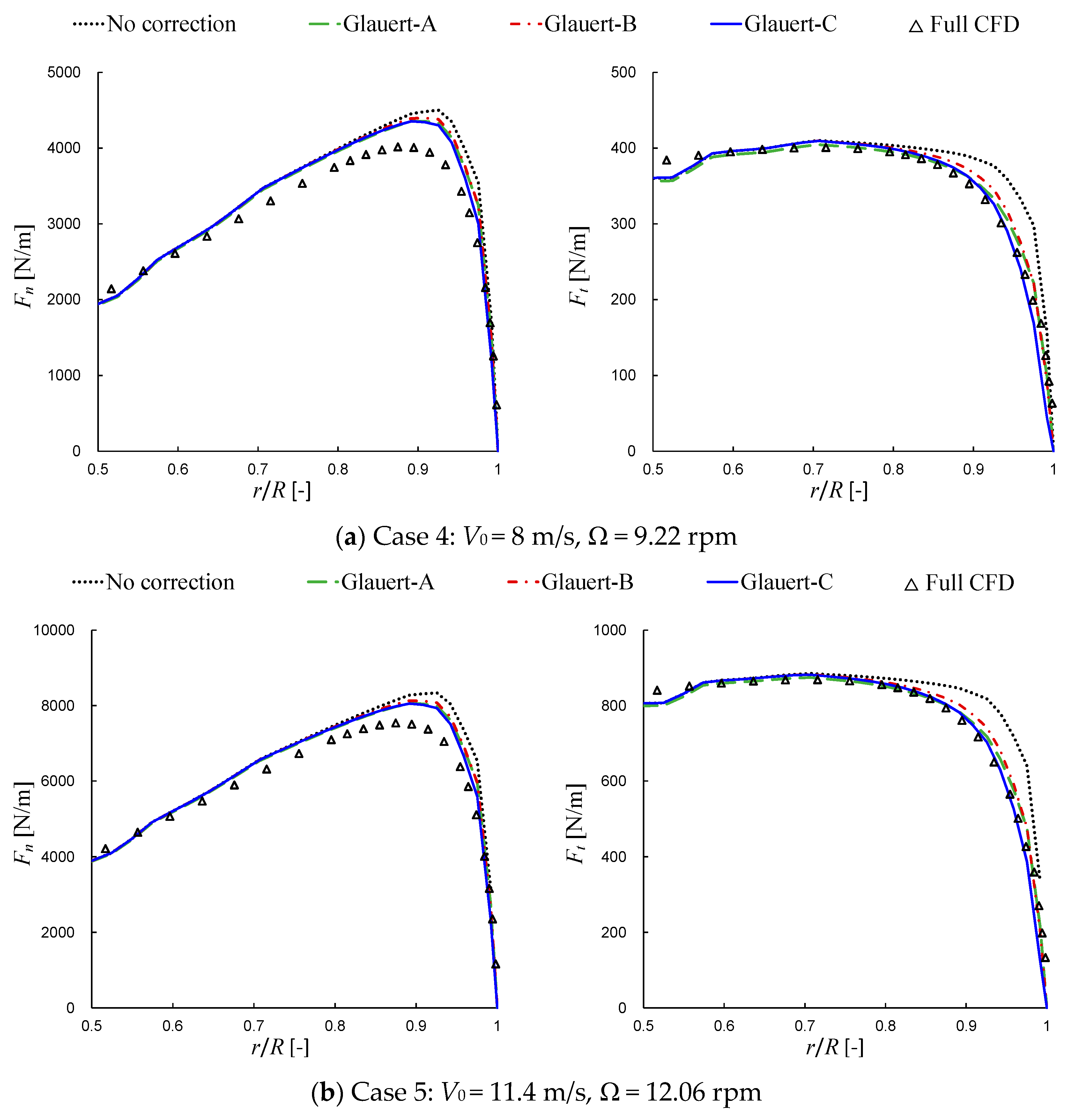
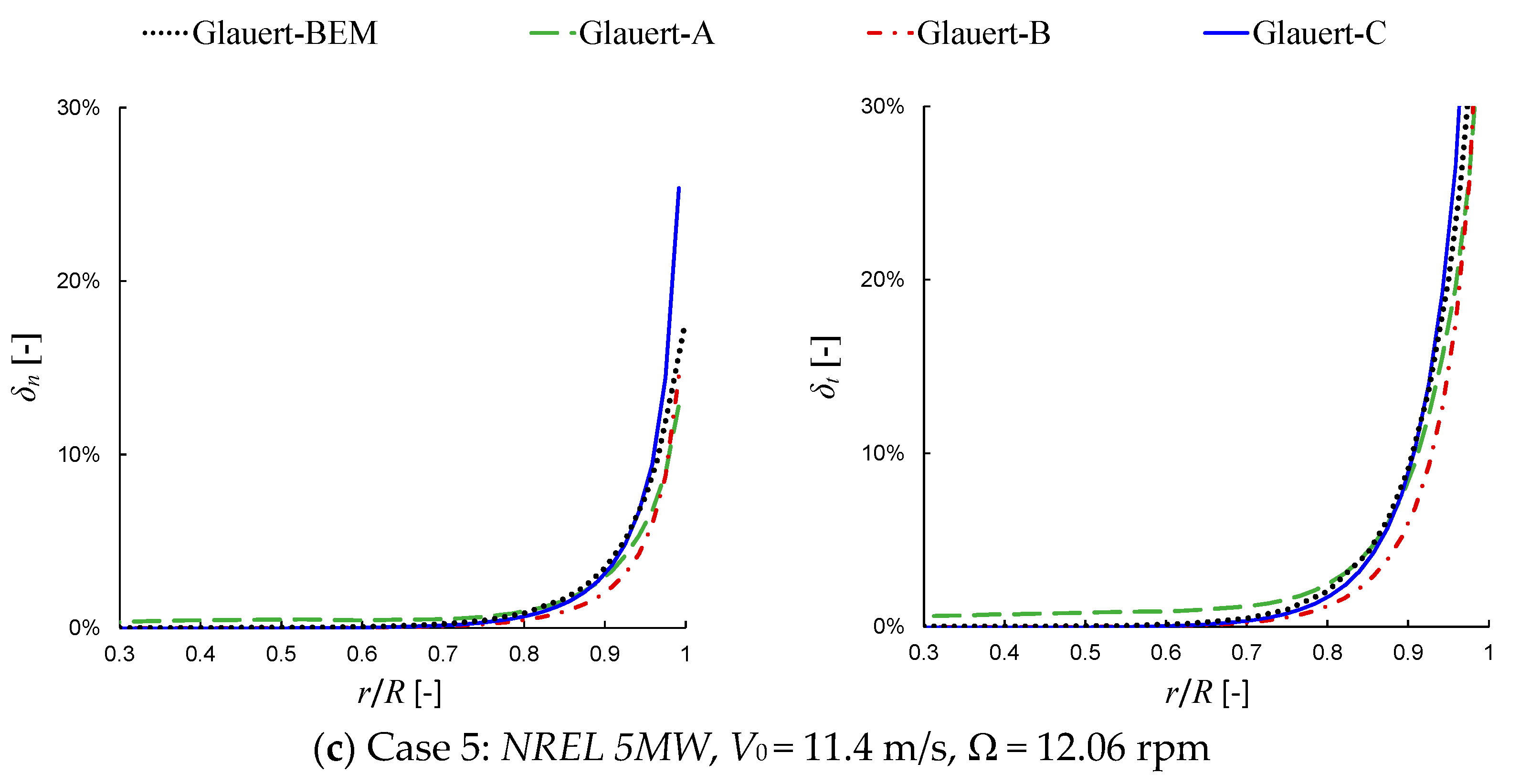
6.1. Results of Glauert-Type Corrections

6.1.1. Glauert-A/B/C Corrections

The blade loads for Cases 1, 2 and 3 are gathered in Figure 4, which represent results obtained from the NREL Phase Ⅵ rotor. The NREL Phase Ⅵ blade has a linear change of chord distribution starting from r = 1.3 m with a constant slope of 0.1. The chord length is 0.358 m at the tip, which is about 48% of the largest chord length in the blade inboard part. Therefore, the loads do not converge to zero without a tip loss correction.

It is noticed that there is a certain degree of difference between the results of the Glauert-A/B/C corrections in the tip region (e.g., at r/R > 0.8). In general, Glauert-C leads to lower loads which are closer to the experimental data, Glauert-A gives results close to, but slightly higher than, those of Glauert-C, while Glauert-B results in relatively higher loads near the tip. Taking the $F_n$ in Figure 4a as an example of quantitative comparison, the relative difference between the results of Glauert-B and Glauert-C is about 4% at r/R = 0.95. The difference in other cases is not larger than this value.

At a wind speed of 7 m/s, all the curves of $F_n$ generally agree with the five experimental data except that at r/R = 0.95 where an overestimation is observed. This overestimation becomes much more remarkable as the wind speed increases to 10 m/s and 13 m/s. At 10 m/s, there is no much difference around r/R = 0.9 between the results with no correction and with the Glauert-type corrections, indicating that almost no effective correction is made here. At 13 m/s, the curves of the Glauert-type corrections even exceed the uncorrected curve in a r/R range of about [0.66, 0.88]. It is clear that the corrections perform much worse at the higher wind speeds as compared with 7 m/s. The overestimation at r/R = 0.95 is also observed in the results for $F_t$, although it looks better to some extent, especially at 7 m/s.

Considering the fact that the Glauert correction was derived based on the potential hypothesis, it is reasonable to believe that the unusually poor performance at the higher wind speed is caused by the flow separation. According to the results of the NREL UAE Phase Ⅵ experiments [50], the angle of attack at most cross-sections of the blade exceeds the linear range of their aerodynamic polar when the wind speed is increased to be higher than 10m/s. Taking the cross-section of r/R = 0.63 as an example, the angles of attack are 5.9°, 11.8°, 16.9° at a wind speed of 7 m/s, 10 m/s, 13 m/s, respectively. The exact operating points for three cases on the lift polar of the S809 airfoil (the airfoil of all cross-sections of the NREL Phase Ⅵ blade) are depicted in Figure 5. It clearly shows that Case 2 and Case 3 are in the nonlinear lift region corresponding to flow separation, while Case 1 is in the linear lift region corresponding to attached flow, which implies that flow separation occurs at 10 m/s and 13 m/s.

The normal and tangential forces along a blade of the NREL 5MW rotor are plotted in Figure 6. As a widely studied virtual rotor, full CFD solutions [33] are often used as the reference data. Although the typical rotating speed of the NREL 5MW rotor is a few times less than the NREL Phase Ⅵ rotor, the resulted tip speed ratio is higher, which is closer to the optimal design point. The blade tip of the NREL 5MW rotor is smoothly sharpened where the slope at the last 4 m is 0.46, and the chord length at the tip is only 4.3% of the largest chord length in the blade inboard part. It can be seen in Figure 6 that the loads at the tip naturally approach to zero even without a tip loss correction.

As a large wind turbine with pitch control, there is no flow separation on the most area of the blade, including the tip. That means the flow pattern ideally keeps the same on the blade as the wind speed increases, which is significantly different from the situation of the NREL Phase Ⅵ rotor. As seen in Figure 6, by increasing the wind speed from 8 m/s to 11.4 m/s, the forces are greatly increased, whereas, their distributions near the tip region remain similar. All the Glauert-A/B/C corrections over-predict the normal forces near the blade tip, whereas, better agreement with the reference data is found for the tangential forces. Such a result is to some extent similar to that of the NREL Phase Ⅵ rotor at 7 m/s. Slight discrepancies are also noticed between the three Glauert-type corrections, and the Glauert-C performs better among them.

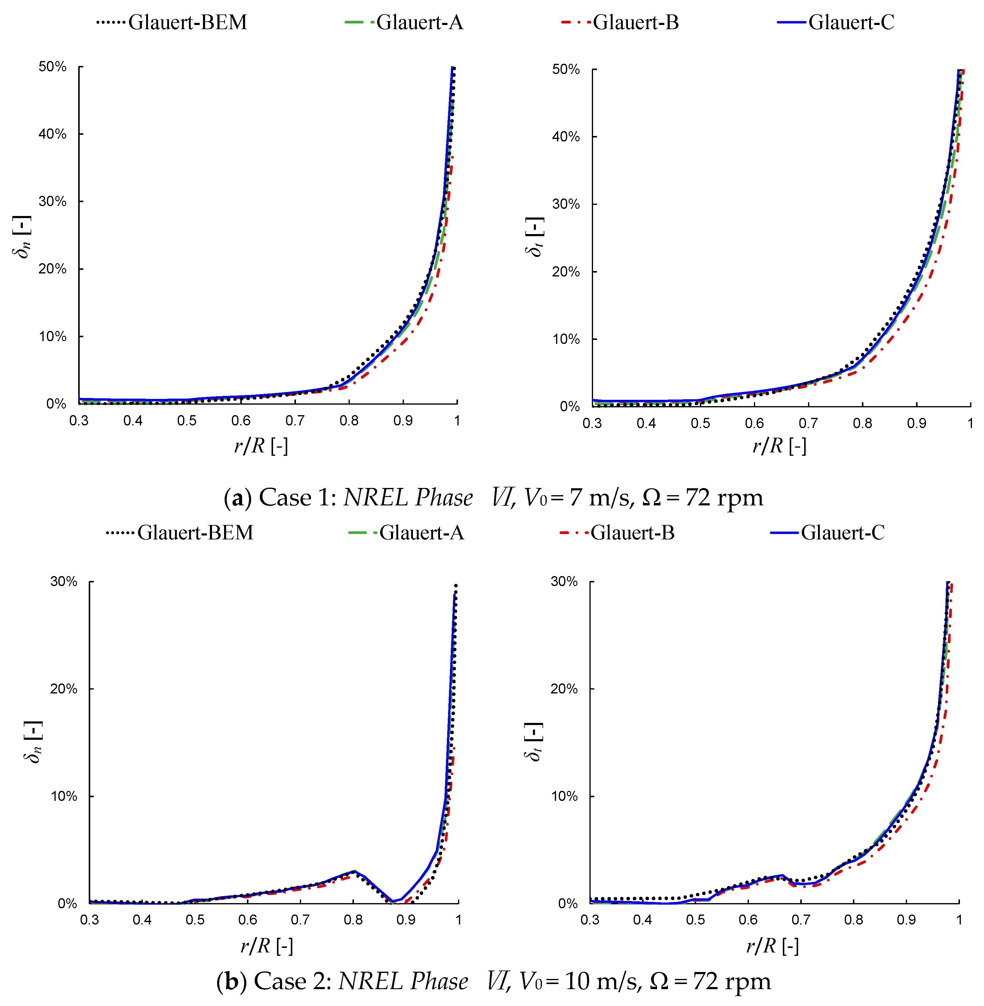
6.1.2. Comparison with BEMT Results

The Glauert tip loss correction was originally proposed for BEMT. As applied to AD/NS simulations, the correction factor F works in a different way. It is worth to mention that the specific difference in the final results would be caused by the transplantation from BEMT to AD/NS. In order to perform a comparison, BEMT computations under the same conditions of the present study are conducted.

The comparisons were shown by percentages, which represent the relative change of blade loads before and after using a tip loss correction,

$${\delta }_n=\frac{F_{n,No}-F_{n,Gl}}{F_{n,No}}\times 100\%,$$

(58)

$${\delta }_t=\frac{F_{t,No}-F_{t,Gl}}{F_{t,No}}\times 100\%,$$

(59)

where $F_{n,No}$ and $F_{n,Gl}$ are the normal forces obtained from computations with no tip loss correction and with the Glauert correction (the standard Glauert correction in BEMT and the Glauert-type corrections in AD/NS), respectively, $F_{t,No}$ and $F_{t,Gl}$ are the corresponding tangential forces.

The above parameters are calculated independently using BEMT and AD/NS. The results are shown in Figure 7 where the Glauert-BEMT denotes the results for the standard Glauert correction used in BEMT, and the Glauert-A/B/C denotes the results for the Glauert-type corrections used in AD/NS. A certain degree of difference between the Glauert-BEMT and the Glauert-A/B/C results is observed. The Glauert-C again shows the best performance, since it is generally most consistent with the Glauert-BEMT, which means the transplantation of the tip loss correction from BEMT to AD/NS does not notably influence its performance. The results for Cases 3 and 4 also agree with the above conclusion, which is not displayed here for simplicity.

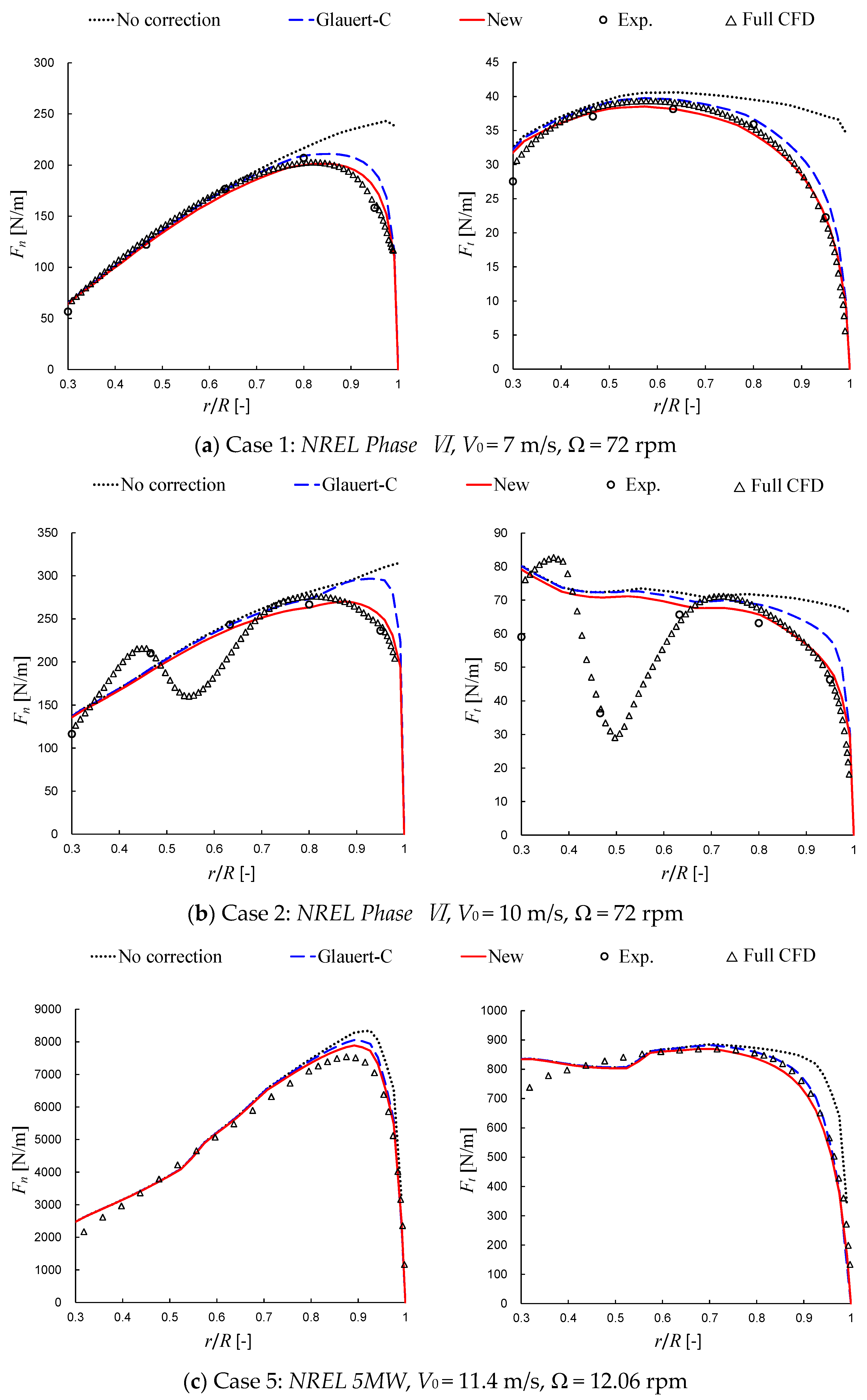
6.2. Results of New Tip Loss Correction

The simplified form (see Section 3.2) of the new correction developed by Zhong et al. [33] is used in the present simulations. The results of blade loads for Cases 1, 2 and 5 are displayed in Figure 8a–c, respectively. Case 1 represents a typical condition of the NREL Phase Ⅵ wind turbine with the fully attached flow on its blades, while Case 2 represents another condition of flow separation (stall). Case 5 represents the rated operating condition of the NREL 5MW wind turbine. The results for Cases 3 and 4 are not displayed here for simplicity. (The performance of the correction in Case 3 is similar to that in Case 2, while the performance in Case 4 is similar to that in Case 5.) The Glauert-C correction, which performs best in Glauert-A/B/C, is compared with the new correction. Full CFD results [33] are employed as the reference data for the NREL 5MW wind turbine. As compensation for the sparse points of the experimental data, full CFD data [8,33] are also employed for the NREL Phase Ⅵ wind turbine.

It is seen in the result of Case 1, as shown in Figure 8a, that the full CFD result achieves the best agreement with the experimental data and the new correction is superior to the Glauert-C correction. As compared to the Glauert-C correction, the overestimation of F_n in the tip region is properly corrected towards the reference data by the new correction. A similar tendency is seen from the tangential force distribution. In Case 2, as shown in Figure 8b, the new correction maintains its accuracy, while the Glauert-C correction produces larger positive error, due to the occurrence of flow separation. The performance of the two corrections is similar to those in BEMT computations [33].

For the NREL 5MW rotor, as shown in Figure 8c, the new correction again makes a better correction to the blade loads in the tip region. The corrected curve of F_n for the new correction is closer to the reference data compared to that for the Glauert-C correction. The difference between the two corrections in tangential force (F_t) is small, and both the corrections can be considered to be doing well.

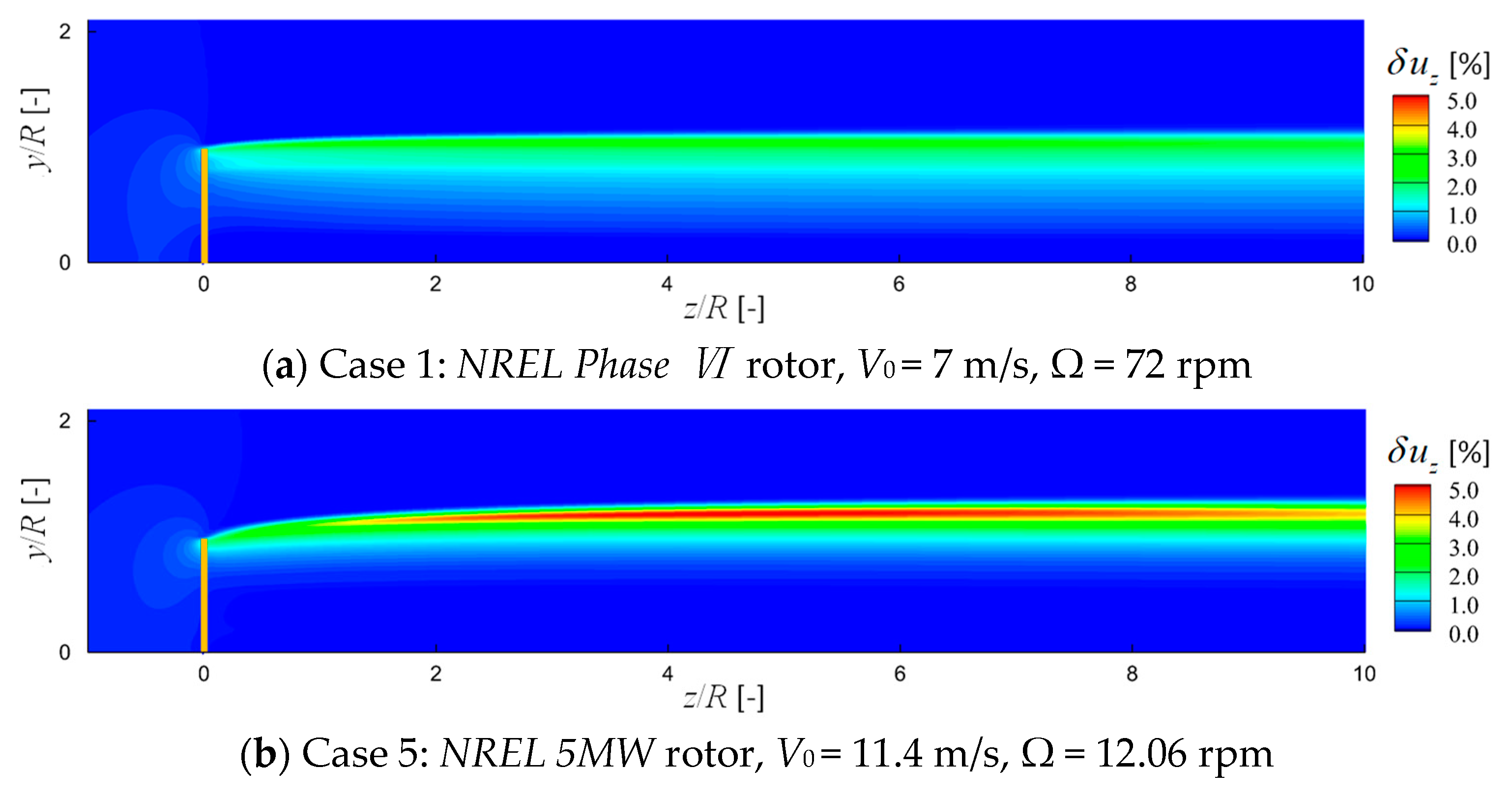
6.3. Comparison of Velocity Field

The blade loads are affected by the local flow around the blade, and the forces consequently modify the flow around the blade and further in the wake. The flowfield simulated by the AD/NS demonstrates how the tip loss corrections affect the velocity field. In order to clearly show the influence of using different tip loss corrections, instead of directly showing the velocity field, the following velocity difference is defined,

$$\delta u_z=\frac{\left|u_{z,new}-u_{z,Gl}\right|}{u_{z,new}}\times 100\%,$$

(60)

where $u_{z,new}$ and $u_{z,Gl}$ are the axial velocity obtained from the simulations using the new tip loss correction and the Glauert-C tip loss correction, respectively.

Figure 9 displays the contours of $\delta u_z$ in the flow field of the studied two rotors, which highlights the influence of the tip loss corrections in terms of changing the velocity field not only around the blade tip, but also in the wake. The influence of $\delta u_z$ is more concentrated near the blade tip in the rotor plane, whereas, the inner part is hardly affected. In the wake, the influence range of $\delta u_z$ tends to cover a wider radial space downstream. The magnitude is even increased in the wake of the NREL 5MW rotor.

7. Conclusions

This work presented AD/NS simulations for the NREL Phase Ⅵ and the NREL 5MW rotors, which represent the typical small size and modern size rotors. The primary purpose of the numerical study is to evaluate the performance of tip loss corrections employed in the AD/NS simulations. Three different implementations of the widely used Glauert tip loss factor F, denoted as Glauert-A/B/C, are discussed and evaluated in the study. In addition, a newly developed tip loss correction is also evaluated. As an extension, the influence of employing different tip loss corrections to the velocity field is studied as well. The following conclusions are drawn from the present study:

• The three different implementations of the Glauert tip loss factor showed a certain degree of difference to each other, although the relative difference in blade loads is generally no more than 4%. The Glauert-C correction, in which the tip loss factor F is directly used to be divided by the interference factors, is recommended for AD/NS simulations, since it gives results closest to the reference data in all the studied cases.
• The performance of the Glauert-C correction in AD/NS was found to be almost equal to that of the standard Glauert correction in BEMT. That provides evidence for the reasonableness of the transplantation of the tip loss correction from BEMT into AD/NS.
• The Glauert-type corrections tend to make an over-prediction of the blade tip loads. In contrast, the new correction showed superior performance in various conditions of the present study.
• A difference in tip loss correction leads to the influence of not only on the blade tip loads, but also on the velocity field around and after the rotor. The range of this influence is observed expanding in the rotor wake. In addition, the magnitude of this influence is found to be increased after the NREL 5 MW rotor.

The above observations help to understand the performance of different tip loss corrections employed in AD/NS simulations. It is indicated that the blade loads, as well as the wake velocity, can be simulated better by choosing the best implementation of the Glauert tip loss factor or employing the new tip loss correction. That is the major contribution of this study.

References

1. Renewables 2019 Global Status Report; REN21: Paris, France, 2019.
2. Shen, W.Z. Special issue on wind turbine aerodynamics. Appl. Sci. 2019, 9, 1725. [Google Scholar] [CrossRef]
3. Hansen, M.O.L. The classical blade element momentum method. In Aerodynamics of Wind Turbines, 3rd ed.; Routledge: Abingdon, UK, 2015; pp. 38–53. [Google Scholar]
4. Sørensen, J.N. General Momentum Theory for Horizontal Axis Wind Turbines; Springer International Publishing Switzerland: Cham, Switzerland, 2016; pp. 123–132. [Google Scholar] [CrossRef]
5. Sumner, J.; Watters, C.S.; Masson, C. CFD in wind energy: The virtual, multiscale wind tunnel. Energies 2010, 3, 989–1013. [Google Scholar] [CrossRef]
6. Sanderse, B.; van er Pijl, S.P.; Koren, B. Review of computational fluid dynamics for wind turbine wake aerodynamics. Wind Energy 2011, 14, 799–819. [Google Scholar] [CrossRef]
7. Rehman, S.; Alam, M.M.; Alhems, L.M.; Rafique, M.M. Horizontal axis wind turbine blade design methodologies for efficiency enhancement—A review. Energies 2018, 11, 506. [Google Scholar] [CrossRef]
8. Zhong, W.; Tang, H.W.; Wang, T.G.; Zhu, C. Accurate RANS simulation of wind turbines stall by turbulence coefficient calibration. Appl. Sci. 2018, 8, 1444. [Google Scholar] [CrossRef]
9. Rodrigues, R.V.; Lengsfeld, C. Development of a computational system to improve wind farm layout, part I: Medel validation and near wake analysis. Energies 2019, 12, 940. [Google Scholar] [CrossRef]
10. Mikkelsen, R.; Sørensen, J.N.; Shen, W.Z. Modelling and analysis of the flow field around a coned rotor. Wind Energy 2001, 4, 121–135. [Google Scholar] [CrossRef]
11. Sharpe, D.J. A general momentum theory applied to an energy-extracting actuator disc. Wind Energy 2004, 7, 177–188. [Google Scholar] [CrossRef]
12. Moens, M.; Duponcheel, M.; Winckelmans, G.; Chatelain, P. An actuator disk method with tip-loss correction based on local effective upstream velocities. Wind Energy 2018, 21, 766–782. [Google Scholar] [CrossRef]
13. Simisiroglou, N.; Polatidis, H.; Ivanell, S. Wind farm power production assessment: Introduction of a new actuator disc method and comparison with existing models in the context of a case study. Appl. Sci. 2019, 9, 431. [Google Scholar] [CrossRef]
14. Sørensen, J.N.; Shen, W.Z. Numerical modeling of wind turbine wakes. J. Fluids Eng. 2002, 124, 393–399. [Google Scholar] [CrossRef]
15. Shen, W.Z.; Zhu, W.J.; Sørensen, J.N. Actuator line/Navier-Stokes computations for the MEXICO rotor: Comparison with detailed measurements. Wind Energy 2012, 15, 811–825. [Google Scholar] [CrossRef]
16. Martínez-Tossas, L.A.; Churchfield, M.J.; Meneveau, C. A highly resolved large-eddy simulation of a wind turbine using an actuator line model with optimal body force projection. J. Phys. Conf. Ser. 2016, 753, 082014. [Google Scholar] [CrossRef]
17. Martínez-Tossas, L.A.; Meneveau, C. Filtered lifting line theory and application to the actuator line model. J. Fluid Mech. 2019, 863, 269–292. [Google Scholar] [CrossRef]
18. Castellani, F.; Vignaroli, A. An application of the actuator disc model for wind turbine wakes calculations. Appl. Energy 2013, 101, 432–440. [Google Scholar] [CrossRef]
19. Wu, Y.T.; Porte-Agel, F. Modeling turbine wakes and power losses within a wind farm using LES: An application to the Horns Rev offshore wind farm. Renew. Energy 2015, 75, 945–955. [Google Scholar] [CrossRef]
20. Sessarego, M.; Shen, W.Z.; van der Laan, M.P.; Hansen, K.S.; Zhu, W.J. CFD simulations of flows in a wind farm in complex terrain and comparisons to measurements. Appl. Sci. 2018, 8, 788. [Google Scholar] [CrossRef]
21. Diaz, G.P.N.; Saulo, A.C.; Otero, A.D. Wind farm interference and terrain interaction simulation by means of an adaptive actuator disc. J. Wind Eng. Ind. Aerodyn. 2019, 186, 58–67. [Google Scholar] [CrossRef]
22. Gargallo-Peiró, A.; Avila, M.; Owen, H.; Prieto-Godino, L.; Folcha, L. Mesh generation, sizing and convergence for onshore and offshore wind farm Atmospheric Boundary Layer flow simulation with actuator discs. J. Comput. Phys. 2018, 375, 209–227. [Google Scholar] [CrossRef]
23. Mao, X.; Sørensen, J.N. Far-wake meandering induced by atmospheric eddies in flow past a wind turbine. J. Fluid Mech. 2018, 846, 190–209. [Google Scholar] [CrossRef]
24. Zhu, W.J.; Shen, W.Z.; Barlas, E.; Bertagnolio, F.; Sørensen, J.N. Wind turbine noise generation and propagation modeling at DTU Wind Energy: A review. Renew. Sustain. Energy Rev. 2018, 88, 133–150. [Google Scholar] [CrossRef]
25. Shen, W.Z.; Zhu, W.J.; Barlas, E; Barlas, E.; Li, Y. Advanced flow and noise simulation method for wind farm assessment in complex terrain. Renew. Energy 2019, 143, 1812–1825. [Google Scholar] [CrossRef]
26. Glauert, H. Airplane propellers. In Aerodynamic Theory; Durand, W.F., Ed.; Dover: New York, NY, USA, 1963; pp. 169–360. [Google Scholar]
27. Branlard, E. Wind Turbine Tip-Loss Corrections. Master’s Thesis, Technical University of Denmark, Lyngby, Denmark, 2011. [Google Scholar]
28. Shen, W.Z.; Mikkelsen, R.; Sørensen, J.N.; Bak, C. Tip loss corrections for wind turbine computations. Wind Energy 2005, 8, 457–475. [Google Scholar] [CrossRef]
29. Sørensen, J.N.; Dag, K.O.; Ramos-Garía, N. A new tip correction based on the decambering approach. J. Phys. Conf. Ser. 2015, 524, 012097. [Google Scholar] [CrossRef]
30. Wood, D.H.; Okulov, V.L.; Bhattacharjee, D. Direct calculation of wind turbine tip loss. Renew. Energy 2016, 95, 269–276. [Google Scholar] [CrossRef]
31. Schmitz, S.; Maniaci, D.C. Methodology to determine a tip-loss factor for highly loaded wind turbines. AIAA J. 2017, 55, 341–351. [Google Scholar] [CrossRef]
32. Wimshurst, A.; Willden, R.H.J. Computatioanl observations of the tip loss mechanism experienced by horizontal axis rotors. Wind Energy 2018, 21, 544–557. [Google Scholar] [CrossRef]
33. Zhong, W.; Shen, W.Z.; Wang, T.; Li, Y. A tip loss correction model for wind turbine aerodynamic performance prediction. Renew. Energy 2020, 147, 223–238. [Google Scholar] [CrossRef]
34. Hand, M.M.; Simms, D.A.; Fingersh, L.J.; Jager, D.W.; Cotrell, J.R.; Schreck, S.; Larwood, S.M. Unsteady Aerodynamics Experiment Phase Vi: Wind Tunnel Test Configurations and Available Data Campaigns; NREL/TP-500-29955; National Renewable Energy Laboratory: Golden, CO, USA, 2001.
35. Jonkman, J.; Butterfield, S.; Musial, W.; Scott, G. Definition of A 5-Mw Reference Wind Turbine for Offshore System Development; Technical Report NREL/TP-500-38060; National Renewable Energy Laboratory: Golden, CO, USA, 2009.
36. Prandtl, L. Applications of Modern Hydrodynamics to Aeronautics; NACA: Washington DC, USA, 1921; No. 116. [Google Scholar]
37. Prandtl, L.; Betz, A. Vier Abhandlungen zur Hydrodynamik und Aerodynamik; Göttingen Nachrichten: Göttingen, Germany, 1927. (In German) [Google Scholar]
38. Ramdin, S.F. Prandtl Tip Loss Factor Assessed. Master’s Thesis, Delft University of Technology, Delft, The Netherlands, 2017. [Google Scholar]
39. Wilson, R.E.; Lissaman, P.B.S. Applied Aerodynamics of Wind Power Machines; NSF/RA/N-74113; Oregon State University: Corvallis, OR, USA, 1974. [Google Scholar]
40. De Vries, O. Fluid Dynamic Aspects of Wind Energy Conversion; AGARD: Brussels, Belgium, 1979; AG-243, Chapter 4; pp. 1–50. [Google Scholar]
41. Sørensen, J.N.; Kock, C.W. A model for unsteady rotor aerodynamics. J. Wind Eng. Ind. Aerodyn. 1995, 58, 259–275. [Google Scholar] [CrossRef]
42. Mikkelsen, R. Actuator Disc Methods Applied to Wind Turbines. Ph.D. Thesis, Technical University of Denmark, Lyngby, Denmark, 2003. [Google Scholar]
43. Shen, W.Z.; Sørensen, J.N.; Mikkelsen, R. Tip loss correction for Actuator/Navier-Stokes computations. J. Sol. Energy Eng. 2005, 127, 209–213. [Google Scholar] [CrossRef]
44. Michelsen, J.A. Basis3d—A Platform for Development of Multiblock PDE Solvers; Technical Report AFM; Technical University of Denmark: Lyngby, Denmark, 1992. [Google Scholar]
45. Sørensen, N.N. General Purpose Flow Solver Applied Over Hills; RISØ-R-827-(EN); Risø National Laboratory: Roskilde, Denmark, 1995. [Google Scholar]
46. Menter, F.R. Two-equation eddy-viscosity turbulence models for engineering applications. AIAA 1994, 32, 1598–1605. [Google Scholar] [CrossRef] [Green Version]
47. Tian, L.L.; Zhu, W.J.; Shen, W.Z.; Sørensen, J.N.; Zhao, N. Investigation of modified AD/RANS models for wind turbine wake predictions in large wind farm. J. Phys. Conf. Ser. 2014, 524, 012151. [Google Scholar] [CrossRef] [Green Version]
48. Prospathopoulos, J.M.; Politis, E.S. Evaluation of the effects of turbulence model enhancements on wind turbine wake predictions. Wind Energy 2011, 14, 285–300. [Google Scholar] [CrossRef]
49. Cao, J.; Zhu, W.; Shen, W; Sørensen, J.N.; Wang, T. Development of a CFD-based wind turbine rotor optimization tool in considering wake effects. Appl. Sci. 2018, 8, 1056. [Google Scholar] [CrossRef] [Green Version]
50. Jonkman, J.M. Modeling of the UAE Wind Turbine for Refinement of FAST_AD; Technical Report NREL/TP-500-34755; National Renewable Energy Lab.: Golden, CO, USA, 2003.
Figure 1. Definition of coordinates and the stream tube through an actuator disc.
Applsci 09 04919 g001
Figure 2. Illustration of the velocity and the aerodynamic force for a blade cross-section.
Applsci 09 04919 g002
Figure 3. Mesh configuration for the Actuator Disc/Navier-Stokes (AD/NS) simulations.
Applsci 09 04919 g003
Figure 4. Normal force F n and tangential force F t along the NREL Phase Ⅵ blade.
Applsci 09 04919 g004aApplsci 09 04919 g004b
Figure 5. Operating points of the cross-section of r/R = 0.63 on the lift polar of the S809 airfoil. (The Reynolds number of the airfoil is 1 × 10⁶ which is close to that of the cross-section).
Applsci 09 04919 g005
Figure 6. Normal force Fn and tangential force Ft along the NREL 5MW blade.
Applsci 09 04919 g006
Figure 7. Distributions of δ n and δ t along a rotor blade.
Applsci 09 04919 g007aApplsci 09 04919 g007b
Figure 8. Normal force Fn and tangential force Ft along the NREL 5MW blade.
Applsci 09 04919 g008
Figure 9. Contours of the axial velocity difference between the results of the new and the Glauert-C tip loss corrections.
Applsci 09 04919 g009