Article

Generative Adversarial Network for Image Super-Resolution Combining Texture Loss

College of Data Science and Software Engineering, Qingdao University, Qingdao 266071, China
*
Author to whom correspondence should be addressed.
Appl. Sci. 2020, 10(5), 1729; https://doi.org/10.3390/app10051729
Submission received: 15 January 2020 / Revised: 27 February 2020 / Accepted: 28 February 2020 / Published: 3 March 2020
(This article belongs to the Special Issue Augmented Reality, Virtual Reality & Semantic 3D Reconstruction)

Abstract

:
Objective: Super-resolution reconstruction is an increasingly important area in computer vision. To alleviate the problems that super-resolution reconstruction models based on generative adversarial networks are difficult to train and contain artifacts in reconstruction results, we propose a novel and improved algorithm. Methods: This paper presented TSRGAN (Super-Resolution Generative Adversarial Networks Combining Texture Loss) model which was also based on generative adversarial networks. We redefined the generator network and discriminator network. Firstly, on the network structure, residual dense blocks without excess batch normalization layers were used to form generator network. Visual Geometry Group (VGG)19 network was adopted as the basic framework of discriminator network. Secondly, in the loss function, the weighting of the four loss functions of texture loss, perceptual loss, adversarial loss and content loss was used as the objective function of generator. Texture loss was proposed to encourage local information matching. Perceptual loss was enhanced by employing the features before activation layer to calculate. Adversarial loss was optimized based on WGAN-GP (Wasserstein GAN with Gradient Penalty) theory. Content loss was used to ensure the accuracy of low-frequency information. During the optimization process, the target image information was reconstructed from different angles of high and low frequencies. Results: The experimental results showed that our method made the average Peak Signal to Noise Ratio of reconstructed images reach 27.99 dB and the average Structural Similarity Index reach 0.778 without losing too much speed, which was superior to other comparison algorithms in objective evaluation index. What is more, TSRGAN significantly improved subjective visual evaluations such as brightness information and texture details. We found that it could generate images with more realistic textures and more accurate brightness, which were more in line with human visual evaluation. Conclusions: Our improvements to the network structure could reduce the model’s calculation amount and stabilize the training direction. In addition, the loss function we present for generator could provide stronger supervision for restoring realistic textures and achieving brightness consistency. Experimental results prove the effectiveness and superiority of TSRGAN algorithm.

1. Introduction

With the popularization of Internet and the development of information technology, the amount of information accepted by human is growing at an explosive rate. Images, videos and audio are the main carriers of information transmission. Related research [1] has pointed out that the information humans receive through vision accounts for 60%~80% of all media information, so visible images are an important way to obtain information. However, the quality of an image is often restricted by hardware equipment such as imaging system and the bandwidth during image transmission process. A low-resolution (LR) image with missing details is eventually presented. The reduction of image resolution will cause a serious decrease in image quality. It will greatly affect people’s visual experience and cannot meet the requirements for image quality performance indicators in industrial production. Therefore, how to obtain high-resolution (HR) images has become an urgent issue.
At present, there are mainly two ways to improve image resolution. The first is to upgrade hardware devices such as image sensors and optics, but this method is too costly and difficult to promote in practical applications. The other is Images Super-Resolution Reconstruction (ISRR) technology which inputs LR images and generates HR images by using machine learning algorithms and digital image processing technology. It has been widely used in fields such as the medical field, communication field, public safety field and remote sensing imaging field for their low cost and practical application values.
The core of original ISRR algorithms are to use the information of neighboring pixels to estimate the pixels of HR images. Typical algorithms include nearest-neighbor interpolation [2], bilinear interpolation [3] and bicubic interpolation [4]. Their disadvantage is that they do not take into account the semantics of entire image, resulting in the lack of high-frequency details in the reconstructed images.
Subsequently, the reconstruction-based ISRR algorithm has been researched and developed. It introduces image priors or constraints between HR and LR images and uses sample information to infer the distribution of real data. Common ISRR algorithms based on reconstruction include convex set projection method [5], iterative back projection method [6] and maximum posterior probability estimation method [7]. Such methods are subject to computational resources and prior conditions when reconstructing images and are unable to produce satisfactory high-quality images.
In order to obtain higher quality reconstructed images, the learning-based ISRR algorithm has been proposed and developed rapidly. It makes full use of information in image sample library to learn the mapping relationship between HR and LR image. According to different design strategies, it is mainly divided into ISRR algorithms based on sparse representation and deep learning. Yang et al. [8] have applied sparse representation theory to ISRR. Tang et al. [9] have proposed a refined local learning scheme to reduce the image artifacts and further improve the image visual quality. Similar algorithms for reconstructing images by learning mapping relationships include Bayesian process estimation [10], statistical learning [11] and linear regression representation algorithm [12].
The matrix or tensor decomposition algorithms that yield low-rank approximations have been developed for various image completion and resolution up-scaling problems. Hatvani et al. [13] have introduced tensor-factorization-based approach which offers a fast solution without the use of known image pairs or strict prior assumptions to solve ISRR task. To tackle the obstacles of low-rank completion methods, Zdunek et al. [14] have proposed to model the incomplete images with overlapping blocks of Tucker decomposition representations.
In recent years, methods based on deep learning have developed rapidly. Since Dong et al. [15] proposed Super-Resolution Convolutional Neural Network (SRCNN) model which first applied Convolutional Neural Networks (CNN) to ISRR, various network architecture designs and training strategies based on CNN [16,17,18,19] have been developed. However, these methods tend to output over-smoothed results without sufficient high-frequency details. In response to the above problem, Johnson et al. [20] have presented to calculate the super-resolution model’s perceptual loss in feature space instead of pixel space. [17,21] have introduced Generative Adversarial Network (GAN) [22] to encourage network to generate more realistic and natural images. Lim et al. [23] have enhanced the deep residual network by removing the Batch Normalization (BN) layers in SRGAN (Generative Adversarial Network for Image Super-Resolution) model. Xintao Wang et al. [24] have used Residual Dense Block (RDB) to constitute the main body of generator network. Although the effect of reconstructed images has been improved, unfortunately, these methods still existed unpleasant artifacts in generated images.
In order to further improve the quality of reconstructed images, this paper presents TSRGAN (Super-Resolution Generative Adversarial Networks Combining Texture Loss) model which is based on GAN. Firstly, we use RDB as the basic unit of generator network and adopt Visual Geometry Group (VGG)19 network as the basic framework of discriminator network. This measure can strengthen the reuse of forward features, reduce the amount of training parameters and control the training direction of reconstruction images. Secondly, four losses are introduced to constitute the total objective function of generator. We propose texture loss to encourage local information matching, enhance perceptual loss by employing the features before activation layer to calculate, optimize adversarial loss based on WGAN-GP (Wasserstein GAN with Gradient Penalty) theory and use content loss to ensure the accuracy of low-frequency information. Experimental results show that the model in this paper has achieved good results, which can generate images with more realistic textures.

2. Related Work

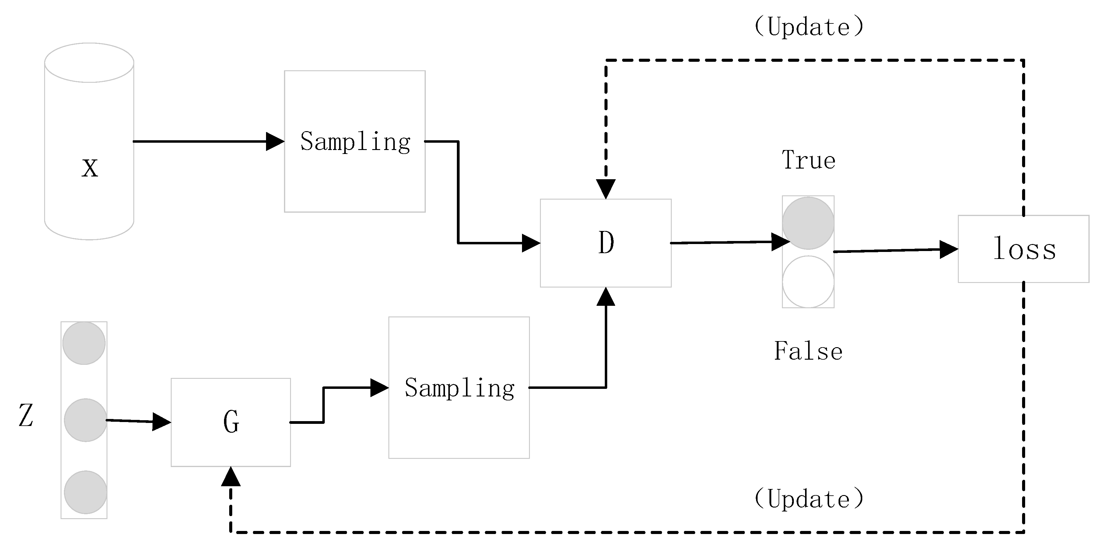
2.1. Generative Adversarial Networks

GAN is a new network framework proposed by Ian Goodfellow et al. [22], it estimates generative model through adversarial process. The zero-sum game is the basic idea of GAN model, the generator (G) and discriminator (D) constitute the main framework of the model. GAN trains network through adversarial learning to achieve Nash equilibrium [25], achieving the goal of estimating data’s potential distribution and generating new data samples.
G and D can be represented by any differentiable function, taking random variable z and real data x as input, respectively. G(z) represents the result generated by G that obeys the distribution of real samples ( p d a t a ) as much as possible. If D’s input is the real sample, D outputs 1, otherwise D outputs 0. D actually acts as a two-classifier. The goal of G is to fool D, so that D could finally give an evaluation result which is closer to 1. G and D oppose each other and iteratively optimize until D can’t distinguish whether the input sample is from G or real data, then it can be considered that the target G has been obtained. The basic framework described in this process is shown in Figure 1. The objective function of GAN is as follows:
m i n   G m a x D V ( D , G ) = E x ~ p d a t a ( x ) [ log D ( x ) ] + E z ~ p z ( z ) ( z ) [ log ( 1 D ( G ( z ) ) ) ]
where G minimizes the objective function to generate samples that can better confuse D, D maximizes the objective function so that D can better distinguish the authenticity of input samples.

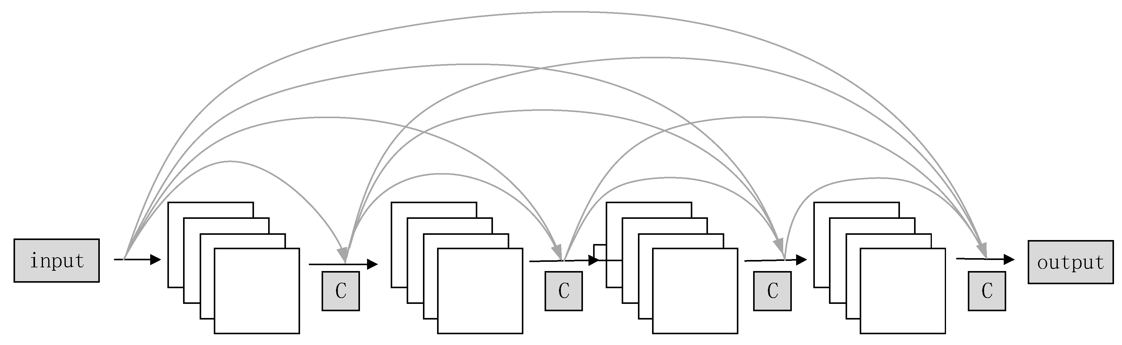
2.2. Dense Convolutional Network

In deep learning networks, the problem of gradient disappearance and gradient dispersion will become more serious as the increase of network layers. The ResNets proposed in [26], the Highway Networks proposed in [27] and the Stochastic depth structure proposed in [28] are all improved networks for the above problems. Although the proposed algorithms are different in network structure and training process, their key point is to create a short path from the forward feature layer to the backward one. Considering the need to ensure the maximum degree of information transmission between different layers, Huang et al. [29] have proposed dense convolutional network (DenseNet), each layer in DenseNet must obtain additional feature inputs from its all feedforward layers and transfer its own feature map to all subsequent layers for effective training. DenseNet has created a deeper and more efficient convolutional network, its dense connection mechanism is shown in Figure 2. The network has obvious advantages in mitigating the disappearance of gradient. Moreover, the structural design that enhances feature propagation and feature reuse can greatly reduce the number of parameters. DenseNet has been widely used in semantic cutting [30], speech recognition [31] and image classification [29].

3. Proposed Methods

This paper uses generative adversarial networks as the main frame, including generator network and discriminator network. The overall structure of TSRGAN is shown in Figure 3. LR image is the generator network’s input, then the convolutional layers are responsible for extracting features. Subsequently, the feature map inputs residual model for non-linear mapping. Then the image is reconstructed through the upsampling layer and convolutional layer. Next, the network outputs the reconstruction result. Finally, we input the fake and real HR images into discriminator network separately, which is responsible for discriminating the authenticity of image.

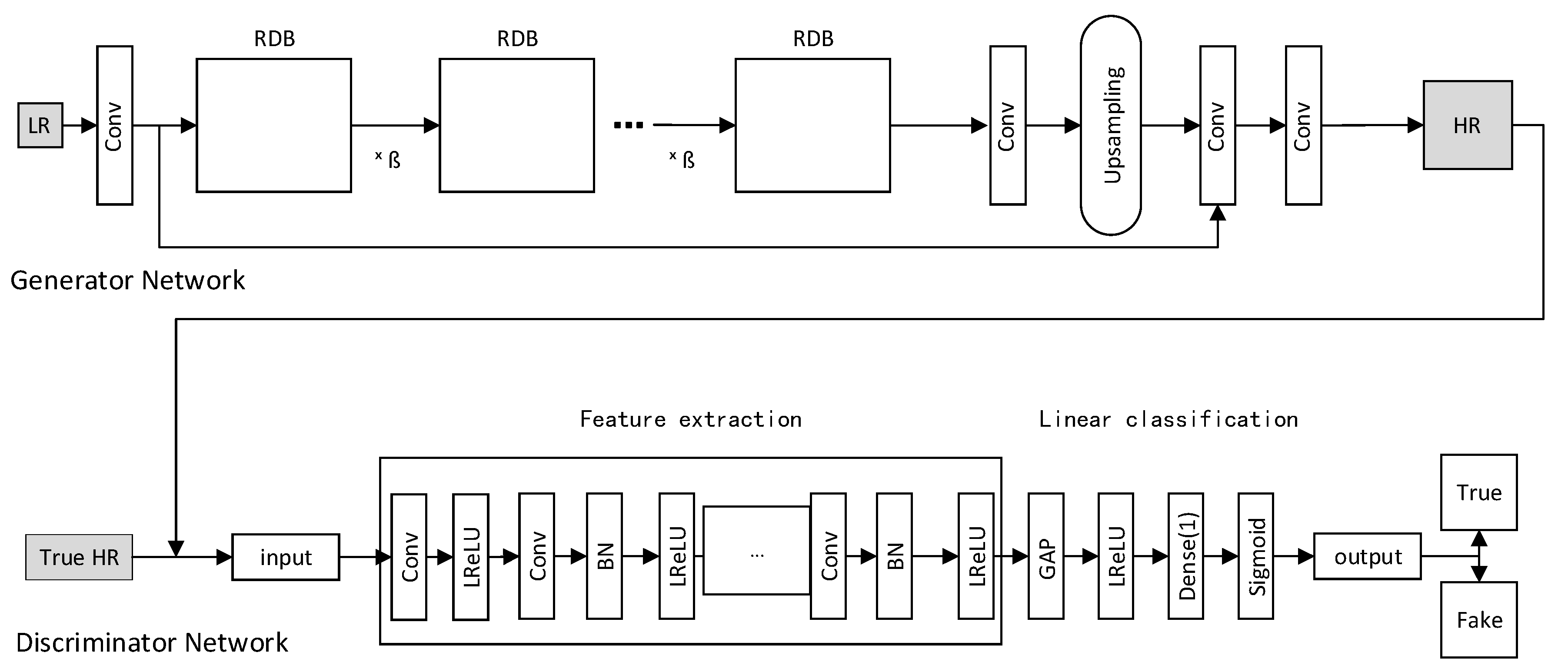
3.1. Network Architecture

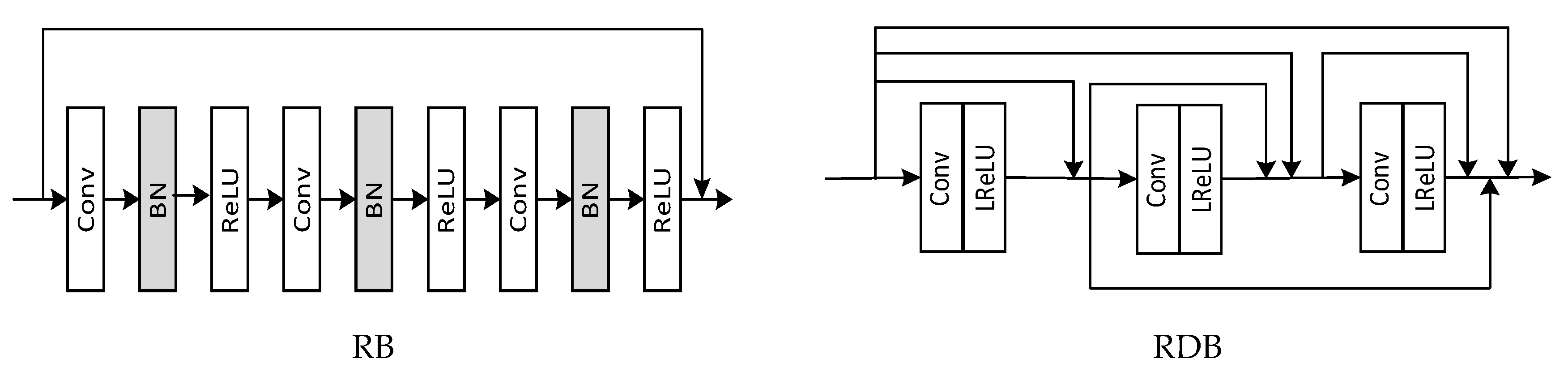
3.1.1. Generator Network

In order to further improve the quality of image reconstruction, this paper improves the network based on SRGAN model. Firstly, all BN layers are removed in SRGAN. BN is easy to introduce artifacts and limit the generalization ability of network. Studies have shown that removing the BN layers can improve reconstruction performance and reduce the computational complexity, such as SR task [23] and deblurring task [32]. Secondly, Leaky Rectified Linear Unit (LeakyReLU) is used instead of Rectified Linear Unit (ReLU) as the network’s non-linear activation function to avoid gradient vanishing problem:
y = max ( 0 , x ) + a min ( 0 , x )
where x is the input, y is the output and a is a constant between 0 and 1. Finally, based on the researches in [31,33,34], it is shown that deep networks and multi-level connections can improve the performance of algorithm. Therefore, we use RDB instead of Residual Block (RB) which is used in SRGAN as the basic network element. RDB has a deeper and more complex structure than RB, it has the advantages of both residual networks and dense connections. It increases the depth of network while improving the reuse of image feature information. Ultimately, it improves the qualities of reconstructed images. The specific structure is shown in Figure 4. Our generator network is a deep model with 36 RDB, it has larger capacity and stronger ability to capture semantic information. Therefor it can reduce the noises of reconstructed images and generate images with more realistic textures.

3.1.2. Discriminator Network

As for the discriminator network, this paper uses the classic VGG19 network as basic architecture, which can be simplified into two modules: feature extraction and linear classification. Feature extraction module includes 16 convolutional layers, after each convolutional layer we use LeakyReLU as the activation function. In addition, the BN layer is used after each convolutional layer except the first one to avoid gradient vanishing problem and enhance the model’s stability. Then the discriminator network needs to judge the input sample image. We use Global Average Pooling (GAP) [35] instead of fully connected layer which is used in most image classification models for fear of reducing the training speed of model and increasing the risk of overfitting. GAP is responsible for calculating the pixel average value of each feature map, and then all the values are sent into sigmoid activation function after linear fusion. Ultimately, network outputs D’s judgement result for the input sample. Training discriminator network helps generator network to restore results that are closer to the ground-truth images.

3.2. Loss Functions

Loss function is an important factor that affects the quality of image reconstruction. In order to restore the high-frequency information and improve the intuitive visual experience of image, this paper uses content loss L c o n , adversarial loss L a d v , perceptual loss L p e r and texture loss L t e x as the objective function of the generator network:
L G = L per + L t e x + λ L a d v + η L c o n
where λ and η are the coefficients which are used to balance different loss functions.

3.2.1. Content Loss

Mean Square Error (MSE) loss is used as the model’s content loss for the sake of ensuring the consistency of low-frequency information between reconstructed image and LR image. It is in charge of optimizing the squared error between pixels corresponding to the generated and real HR images. Reducing the distance between pixels can more quickly and effectively ensure the accuracy of the reconstructed image information, so that the results could get a higher value of peak signal to noise ratio.
L con = L M S E ( θ ) = 1 N i = 1 N | | I i H G ( I i L , θ ) | | 2
where I i H represents the real HR image, I i L represents the LR image, N represents the number of training samples and G ( x , θ ) represents the mapping function between LR and HR images learned by the generator network.

3.2.2. Adversarial Loss

Based on the adversarial game mechanism between generator and discriminator network, the discriminator network needs to product the probability of image which is output by generator network being true or false. To maximize the probability that the reconstructed image deceives D, we adopt the adversarial loss proposed in WGAN-GP [36] model to replace the one proposed in GAN model. Improved L a d v penalizes D for the gradient of input, it can help stable training of GAN architecture and generate higher quality samples with faster convergence speed with little need for tuning of hyperparameters.
L a d v = E x ~ p G [ D ( x ) ] E x ~ p d a t a [ D ( x ) ] + λ E x ~ p e n a l t y [ ( | | x D ( x ) | | 1 ) 2 ]

3.2.3. Perceptual Loss

In order to generate images with more accurate brightness and realistic textures, L p e r based on VGG network is set to be calculated using feature layer information before activation layer instead of after it. It is defined on the activation layer of the pre-trained deep network to minimize the Euclidean distance between two activation features:
L p e r = 1 W i j H i j x = 1 W i j y = 1 H i j ( ϕ i j ( I H R ) x , y ϕ i j ( G ( I L R ) ) x , y ) 2
where, W i j and H i j describe the dimensions of the respective feature maps within the VGG network, i j indicates the feature map obtained by the j-th convolution (after activation) before the i-th maxpooling layer within the network. The improved L p e r overcomes two drawbacks of the original design: First, the activated features are very sparse, especially after a very deep network, the sparse activation provides weak supervision and thus leads to inferior performance. Second, using features after activation also causes inconsistent reconstructed brightness compared with the ground-truth image.

3.2.4. Texture Loss

Although perceptual loss can improve the quality of reconstructed image as a whole, it still has the problem of introducing unnecessary high-frequency structures. We propose to incorporate texture loss presented in [21] to constitute the total loss function of G. L t e x encourages local matching of texture information, it extracts feature maps generated by the intermediate layer of convolutional network of generator and discriminator network. Then it calculates the corresponding gram matrix. Finally, L2 loss function is used to calculate texture loss for the obtained Gram matrix values:
L t e x = | | G ( ϕ ( I g e n ) G ( ϕ ( I H R ) ) | | 2 2
where I g e n indicates images that are reconstructed by generator, G indicates the Gram matrix, G ( F ) = F F T . Texture loss provides strong supervision to further reduce visually incredible artifacts and produce more realistic textures.

4. Experiments and Results

4.1. Experimental Details

The experimental platform we use is NVIDIA GeForceMX150, Intel (R) Core (TM) i7-8550U [email protected], 8 GB RAM, the compilation software we use are pycharm2017 and MATLAB 2018a, and the pytorch deep learning toolbox is used to build and train the network. This paper uses DIV2K dataset, which consists of 800 training images, 100 validation images and 100 testing images. We augment the training data with random horizontal flips and 90 rotations. We perform experiments on three widely used benchmark datasets Set5 [37], Set14 [38] and BSD100 [39]. All experiments are performed with a scale factor of 4× between low- and high-resolution images. The mini-batch size is set to 16. The spatial size of cropped HR patch is 128 × 128.
The training process is divided into two stages. First, we train a generative model with L 1 loss as the objective function. Then, we use the initially trained model as the initialization of G. The generator is trained using the loss function in Equation (3). The initial learning rate is set to 1 × 10⁻⁴. For optimization, we use Adam with β1 = 0.9, β2 = 0.999. We alternately update the generator and discriminator network until the model converges. In addition, we introduce a residual scaling [40] strategy which scales down the residuals by multiplying a constant β between 0 and 1 before adding them to the main path to prevent instability. β is set to 0.2 in this paper.
For accurately evaluating image quality and proving the effectiveness of algorithm, Peak Signal to Noise Ratio (PSNR) and Structural Similarity Index (SSIM) are adopted as image quality evaluation indicators. μ X and μ Y represent the mean values of images X and Y, σ X and σ Y represent the standard deviations of images X and Y and σ X Y represents the covariance of images X and Y. PSNR is responsible for measuring the distortion of images from the difference in pixels, and SSIM is responsible for measuring the similarity of the images from the brightness, contrast and structure. The larger the two values, the closer the reconstruction result is to the ground-truth image.
P S N R = 10 × log 10 255 2 × W × H × C i = 1 W j = 1 H z = 1 C [ x ¯ ( i , j ) x ( i , j ) ] 2 + 1 × 10 9
S S I M ( X , Y ) = ( 2 μ X μ Y + C 1 ) ( 2 σ X Y + C 2 ) ( μ X 2 + μ Y 2 + C 1 ) ( σ X 2 + σ Y 2 + C 2 )

4.2. Experimental Results

4.2.1. Quantitative Evaluation

We have performed super-resolution experiments on Set5 and Set14 to analyze the effects of introducing RDB structure, L t e x and improving initial L a d v , L p e r on super-resolution performance. The PSNR values of different model variants are shown in Table 1. It can be observed that each of the above four enhanced measures can improve the super-resolution performance of the network, and the effect is the best when all of them are used. In addition, we have adopted different values for λ and η in Equation (3) and performed experiments on Set5. The results have shown that the reconstruction effect is the best when λ = 3 × 10⁻³ and η = 2 × 10⁻². Table 2 presents the average PSNR results on Set5 dataset.
For fair comparison, the SISR methods in comparison are Bicubic [4], ScSR [8], SRGAN [17], EDSR [23] and ESRGAN [24], all these methods are tested on Set5, Set14 and BSD100, respectively. Average PSNR/SSIM values on different datasets with those methods are recorded in Table 3, and the total running time with those methods on different datasets is recorded in Table 4. It can be seen from Table 3 that the performance of TSRGAN on PSNR is generally better than other algorithms. Except that the SSIM value is slightly lower than ESRGAN 0.009 on Set14, it is also superior than other algorithms. Note that Table 4 shows the results that Bicubic consumes the shortest time for it only has interpolation operations. ScSR spends longer time for learning sparse representation dictionaries between the LR and HR image patch pairs. SRGAN, EDSR, ESRGAN and TSRGAN models all need longer time to train for they have extensive convolutional layers. SRGAN has the slowest reconstruction speed because the BN layer is not removed in the network structure, while TSRGAN is slightly slower than EDSR and ESRGAN due to the introduction of deeper network and texture loss. Synthesizing Table 3 and Table 4, TSRGAN obviously improves PSNR and SSIM indicators for measuring the quality of image reconstruction without losing too much speed, which verifies its effectiveness and superiority.

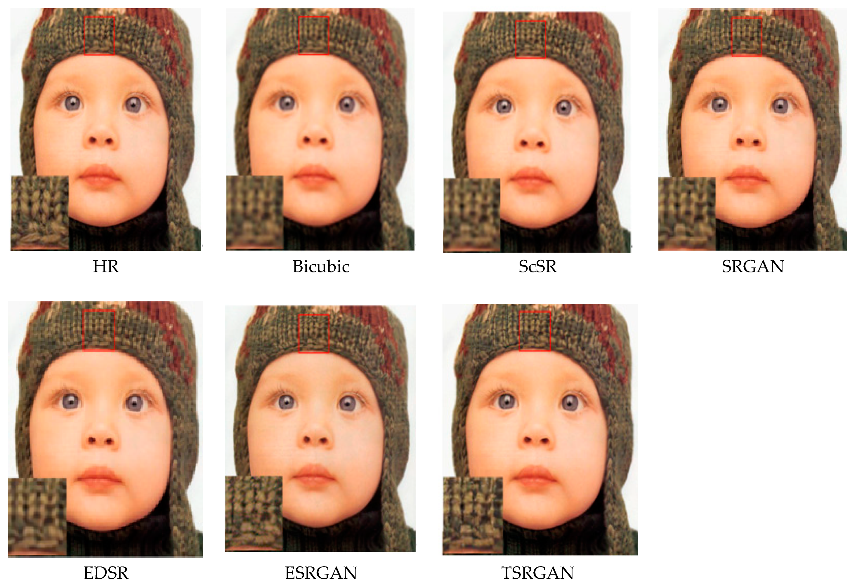
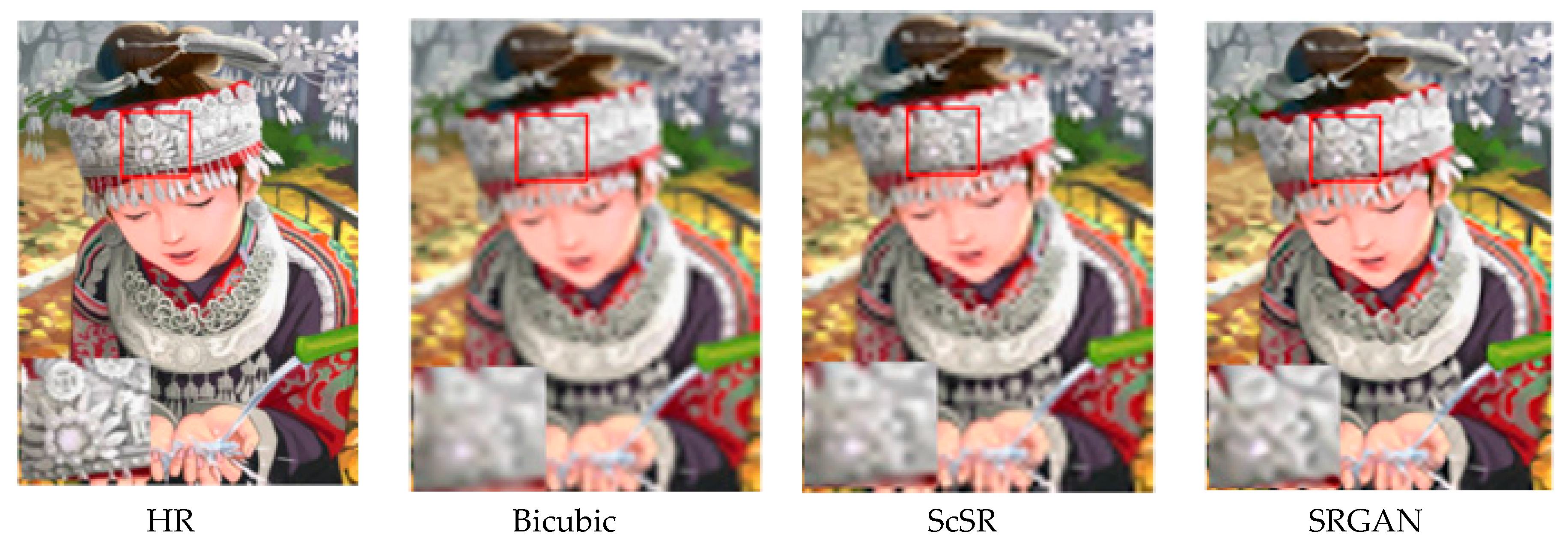
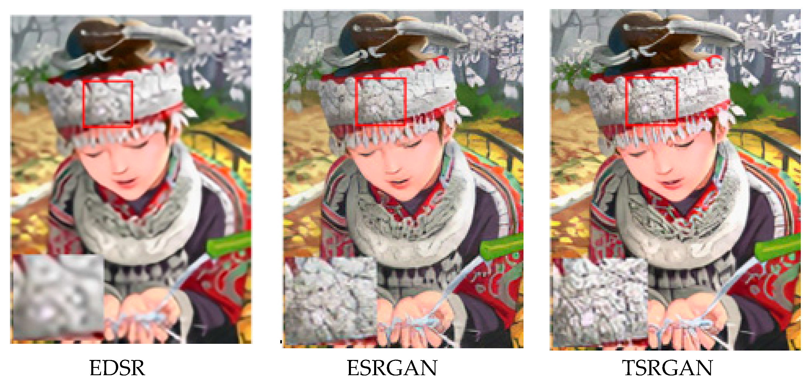
4.2.2. Qualitative Evaluation

In order to ensure the contrast effect, we select an image from datasets Set5 and Set14, respectively. The actual reconstruction results of each algorithm are shown in Figure 5 and Figure 6. Comparing the reconstruction results, it can be observed that the reconstruction details of Bicubic and ScSR are too few, and the generated images are very blurred. Although SRGAN and EDSR have restored some high-frequency information, the edge sharpening effect is poor. The overall effect of ESRGAN is better, but it has introduced unpleasant artifacts and noises. The reconstruction results of TSRGAN are superior to other algorithms in terms of sharpness and detail. As can be seen from enlarged details in Figure 5, TSRGAN can generate a clearer and more natural hat textures. According to Figure 6, it can be observed that TSRGAN has generated image with more accurate brightness information and more pleasing texture details.

5. Conclusions

Based on the generative adversarial network framework, we have described a super-resolution model TSRGAN. We have designed the method of removing BN layers and introducing residual dense blocks to deepen the structure of generator network. In addition, we have used WGAN-GP to improve adversarial loss to provide stronger and more effective supervision for model training. Moreover, we have enhanced perceptual loss by using the features before activation layer, which offer stronger supervision and thus restore more accurate brightness and realistic textures. Finally, we have cited texture loss which encourages to match local texture details to achieve better outcomes. The experimental results show that our method makes the average PSNR of reconstructed images reach 27.99 dB and the average SSIM reach 0.778 without losing too much speed, which is superior to other comparison algorithms in objective evaluation index. TSRGAN has significantly improved subjective visual evaluations such as brightness information and texture details, this further proves that our algorithm can reconstruct more realistic images. In future research work, we will consider super-resolution reconstruction of images in specific fields or scenes to improve the quality of image generation.

Author Contributions

Writing—original draft, Y.J.; Writing—review & editing, Y.J. and J.L. All authors have read and agreed to the published version of the manuscript.

Funding

This research was funded by Key Research and Development Plan - Major Scientific and Technological Innovation Projects of ShanDong Province (2019JZZY020101).

Acknowledgments

This study is undertaken within the framework of SRGAN. Furthermore, the authors wish to thank Zhao Junli and Yang Chun for their helpful comments and encouragement for many aspects of the paper, and we wish to thank Dong Yuehang for helping with the ISRR experimental environment support.

Conflicts of Interest

We declare that we have no conflict of interest.

References

  1. Gonzalez, R.; Woods, R.E. Digital Image Processing. Up. Saddle River Nj Pearson Hall. 2002, 28, 290–291. [Google Scholar]
  2. Schultz, R.R.; Stevenson, R.L. A Bayesian approach to image expansion for improved definition. IEEE Trans. Image Process. 1994, 3, 233–242. [Google Scholar] [CrossRef] [PubMed]
  3. Gribbon, K.T.; Bailey, D.G. A novel approach to real-time bilinear interpolation. In Proceedings of the DELTA, Second IEEE International Workshop on Electronic Design, Test and Applications, Perth, WA, Australia, 28–30 January 2004; pp. 126–131. [Google Scholar]
  4. Zhang, L.; Wu, X. An edge-guided image interpolation algorithm via directional filtering and data fusion. IEEE Trans. Image Process. 2006, 15, 2226–2238. [Google Scholar] [CrossRef] [PubMed] [Green Version]
  5. Jung, S.W.; Kim, T.H.; Ko, S.J. A novel multiple image deblurring technique using fuzzy projection onto convex sets. IEEE Signal Process. Lett. 2009, 16, 192–195. [Google Scholar] [CrossRef]
  6. Nayak, R.; Harshavardhan, S.; Patra, D. Morphology based iterative back-projection for super-resolution reconstruction of image. In Proceedings of the 2014 2nd International Conference on Emerging Technology Trends in Electronics, Communication and Networking, Surat, India, 26–27 December 2014; pp. 1–6. [Google Scholar]
  7. Sun, D.; Gao, Q.; Lu, Y.; Huang, Z.; Li, T. A novel image denoising algorithm using linear Bayesian MAP estimation based on sparse representation. Signal Process. 2014, 100, 132–145. [Google Scholar] [CrossRef]
  8. Yang, J.; Wright, J.; Huang, T.; Ma, Y. Image super-resolution via sparse representation. IEEE Process. IEEE Trans. Image Process. 2010, 19, 2861–2873. [Google Scholar] [CrossRef] [PubMed]
  9. Tang, S.; Xiao, L.; Liu, P. Single image super-resolution method via refined local learning. J. Shanghai Jiaotong Univ. (Sci.) 2015, 20, 26–31. [Google Scholar] [CrossRef]
  10. He, L.; Qi, H.; Zaretzki, R. Beta process joint dictionary learning for coupled feature spaces with application to single image super-resolution. In Proceedings of the IEEE Conference on Computer Vision and Pattern recognition, Portland, ON, USA, 23–28 June 2013; pp. 345–352. [Google Scholar]
  11. Peleg, T.; Elad, M. A statistical prediction model based on sparse representations for single image super-resolution. IEEE Trans. Image Process. 2014, 23, 2569–2582. [Google Scholar] [CrossRef] [PubMed]
  12. Hu, Y.; Wang, N.; Tao, D.; Gao, X.; Li, X. SERF: A simple, effective, robust, and fast image super-resolver from cascaded linear regression. IEEE Trans. Image Process. 2016, 25, 4091–4102. [Google Scholar] [CrossRef] [PubMed]
  13. Hatvani, J.; Basarab, A.; Tourneret, J.Y.; Gyöngy, M.; Kouamé, D. A Tensor Factorization Method for 3-D Super Resolution with Application to Dental CT. IEEE Trans. Med. Imaging 2018, 38, 1524–1531. [Google Scholar] [CrossRef] [PubMed]
  14. Zdunek, R.; Sadowski, T. Image Completion with Hybrid Interpolation in Tensor Representation. Appl. Sci. 2020, 10, 797. [Google Scholar] [CrossRef] [Green Version]
  15. Dong, C.; Loy, C.C.; He, K.; Tang, X. Image Super-Resolution Using Deep Convolutional Networks. IEEE Trans. Pattern Anal. Mach. Intell. 2016, 38, 295–307. [Google Scholar] [CrossRef] [PubMed] [Green Version]
  16. Kim, J.; Kwon Lee, J.; Mu Lee, K. Accurate image super-resolution using very deep convolutional networks. In Proceedings of the IEEE Conference on Computer Vision and Pattern Recognition, Las Vegas, NV, USA, 27–30 June 2016; pp. 1646–1654. [Google Scholar]
  17. Ledig, C.; Theis, L.; Huszar, F.; Caballero, J.; Cunningham, A.; Acosta, A.; Aitken, A.; Tejani, A.; Totz, J.; Wang, Z.H.; et al. Photo-realistic single image super-resolution using a generative adversarial network. In Proceedings of the IEEE Conference on Computer Vision and Pattern Recognition, Honolulu, HI, USA, 21–26 July 2017; pp. 4681–4690. [Google Scholar]
  18. Lai, W.S.; Huang, J.B.; Ahuja, N.; Yang, M. Deep laplacian pyramid networks for fast and accurate super-resolution. In Proceedings of the IEEE Conference on Computer Vision and Pattern Recognition, Honolulu, HI, USA, 21–26 July 2017; pp. 624–632. [Google Scholar]
  19. Tai, Y.; Yang, J.; Liu, X. Image super-resolution via deep recursive residual network. In Proceedings of the IEEE Conference on Computer Vision and Pattern Recognition, Honolulu, HI, USA, 21–26 July 2017; pp. 3147–3155. [Google Scholar]
  20. Johnson, J.; Alahi, A.; Fei-Fei, L. Perceptual losses for real-time style transfer and super-resolution. In Proceedings of the European Conference on Computer Vision, Amsterdam, The Netherland, 8–16 October 2016; Springer: Berlin/Heidelberg, Germany, 2016; pp. 694–711. [Google Scholar]
  21. Sajjadi, M.S.M.; Scholkopf, B.; Hirsch, M. Enhancenet: Single image super-resolution through automated texture synthesis. In Proceedings of the IEEE International Conference on Computer Vision, Venice, Italy, 22–29 October 2017; pp. 4491–4500. [Google Scholar]
  22. Goodfellow, I.; Pouget-Abadie, J.; Mirza, M.; Xu, B.; Warde-Farley, D.; Ozair, S.; Courville, A.; Bengio, Y. Generative adversarial nets. In Proceedings of the Advances in Neural Information Processing Systems, Montreal, QC, Canada, 8–13 December 2014; pp. 2672–2680. [Google Scholar]
  23. Lim, B.; Son, S.; Kim, H.; Nah, S.; Lee, K.M. Enhanced deep residual networks for single image super-resolution. In Proceedings of the IEEE Conference on Computer Vision and Pattern Recognition Workshops, Honolulu, HI, USA, 21–26 July 2017; pp. 136–144. [Google Scholar]
  24. Wang, X.; Yu, K.; Wu, S.; Gu, J.; Liu, Y.; Dong, C.; Loy, C.C.; Qiao, Y.; Tang, X. Esrgan: Enhanced super-resolution generative adversarial networks. In Proceedings of the European Conference on Computer Vision (ECCV), Munich, Germany, 8–14 September 2018. [Google Scholar]
  25. Ratliff, L.J.; Burden, S.A.; Sastry, S.S. Characterization and computation of local nash equilibria in continuous games. In Proceedings of the 2013 51st Annual Allerton Conference on Communication, Control, and Computing (Allerton), Monticello, IL, USA, 2–4 October 2013; IEEE: Piscataway, NJ, USA, 2013; pp. 917–924. [Google Scholar]
  26. He, K.; Zhang, X.; Ren, S.; Sun, J. Identity mappings in deep residual networks. In Proceedings of the European Conference on Computer Vision, Amsterdam, The Netherland, 8–16 October 2016; Springer: Berlin/Heidelberg, Germany, 2016; pp. 630–645. [Google Scholar]
  27. Srivastava, R.K.; Greff, K.; Schmidhuber, J. Training very deep networks. In Proceedings of the Advances in Neural Information Processing Systems, Montreal, QC, Canada, 7–12 December 2015; pp. 2377–2385. [Google Scholar]
  28. Huang, G.; Sun, Y.; Liu, Z.; Sedra, D.; Weinberger, K. Deep networks with stochastic depth. In Proceedings of the European Conference on Computer Vision, Amsterdam, The Netherland, 8–16 October 2016; Springer: Berlin/Heidelberg, Germany, 2016; pp. 646–661. [Google Scholar]
  29. Huang, G.; Liu, Z.; Van Der Maaten, L.; Weinberger, K.Q. Densely connected convolutional networks. In Proceedings of the IEEE Conference on Computer Vision and Pattern Recognition, Honolulu, HI, USA, 21–26 July 2017; pp. 4700–4708. [Google Scholar]
  30. Jégou, S.; Drozdzal, M.; Vazquez, D.; Romero, A.; Bengio, Y. The one hundred layers tiramisu: Fully convolutional densenets for semantic segmentation. In Proceedings of the IEEE Conference on Computer Vision and Pattern Recognition Workshops, Honolulu, HI, USA, 21–26 July 2017; pp. 11–19. [Google Scholar]
  31. Park, S.; Jeong, Y.; Kim, H.S. Multi-resolution DenseNet based acoustic models for reverberant speech recognition. Phon. Speech Sci. 2018, 10, 33–38. [Google Scholar] [CrossRef]
  32. Nah, S.; Hyun Kim, T.; Mu Lee, K. Deep multi-scale convolutional neural network for dynamic scene deblurring. In Proceedings of the IEEE Conference on Computer Vision and Pattern Recognition, Honolulu, HI, USA, 21–26 July 2017; pp. 3883–3891. [Google Scholar]
  33. Zhang, Y.; Tian, Y.; Kong, Y.; Zhong, B.; Fu, Y. Residual densenet work for image super-resolution. In Proceedings of the IEEE Conference on Computer Vision and Pattern Recognition, Salt Lake City, UT, USA, 18–23 June 2018; pp. 2472–2481. [Google Scholar]
  34. Zhang, Y.; Li, K.; Li, K.; Wang, L.; Zhong, B.; Fu, Y. Image super-resolution using very deep residual channel attention networks. In Proceedings of the European Conference on Computer Vision (ECCV), Munich, Germany, 8–14 September 2018; pp. 286–301. [Google Scholar]
  35. Szegedy, C.; Liu, W.; Jia, Y.; Sermanet, P.; Reed, S.; Anguelov, D.; Erhan, D.; Vanhoucke, V.; Rabinovich, A. Going deeper with convolutions. In Proceedings of the IEEE Conference on Computer Vision and Pattern Recognition, Boston, MA, USA, 7–12 June 2015; pp. 1–9. [Google Scholar]
  36. Gulrajani, I.; Ahmed, F.; Arjovsky, M.; Dumoulin, V.; Courville, A. Improved training of wasserstein gans. In Proceedings of the Advances in Neural Information Processing Systems, Long Beach, CA, USA, 4–9 December 2017; pp. 5767–5777. [Google Scholar]
  37. Bevilacqua, M.; Roumy, A.; Guillemot, C.; Alberi Morel, M.-L. Low-Complexity Single-Image Super-Resolution based on Nonnegative Neighbor Embedding. In Proceedings of the Acoustics, Speech and Signal Processing (ICASSP), Kyoto, Japan, 25–30 March 2012. [Google Scholar]
  38. Zeyde, R.; Elad, M.; Protter, M. On single image scale-up using sparse-representations. In Proceedings of the International Conference on Curves and Surfaces, Avignon, France, 24–30 June 2010; Springer: Berlin/Heidelberg, Germany, 2010; pp. 711–730. [Google Scholar]
  39. Martin, D.; Fowlkes, C.; Tal, D.; Malik, J. A database of human segmented natural images and its application to evaluating segmentation algorithms and measuring ecological statistics. In Proceedings of the Eighth IEEE International Conference on Computer Vision, ICCV, Vancouver, BC, Canada, 7–14 July 2001; Volume 2, pp. 416–423. [Google Scholar]
  40. Szegedy, C.; Ioffe, S.; Vanhoucke, V.; Alemi, A. Inception-v4, inception-resnet and the impact of residual connections on learning. In Proceedings of the Thirty-First AAAI Conference on Artificial Intelligence, San Francisco, CA, USA, 4–9 February 2017. [Google Scholar]
Figure 1. The basic framework of Generative Adversarial Network (GAN).
Applsci 10 01729 g001
Figure 2. DenseNet’s dense connection mechanism.
Applsci 10 01729 g002
Figure 3. Architecture of generator and discriminator network.
Applsci 10 01729 g003
Figure 4. The structure of Residual Block (RB) and Residual Dense Block (RDB).
Applsci 10 01729 g004
Figure 5. Reconstruction effects from the selected algorithms on Set5 dataset.
Applsci 10 01729 g005
Figure 6. Reconstruction effects from the selected algorithms on Set14 dataset.
Applsci 10 01729 g006aApplsci 10 01729 g006b
Table 1. Average PSNR (dB) of different super-resolution models on Set5 and Set14 datasets.
RDB L a d v L p e r L t e x Set5Set14
××××30.3727.02
×××31.2227.98
××31.5428.27
×31.8328.39
32.3828.73
Table 2. The average PSNR (dB) results on Set5 dataset when λ and η take different values.
λ1 × 1032 × 1033 × 1034 × 1035 × 103
η
1× 10−232.3132.3432.3632.3532.36
2 × 10−232.3232.3532.3832.3632.35
3× 10−232.3132.3332.3632.3432.32
Table 3. Average PSNR (dB)/SSIM comparison of different SR algorithms on Set5, Set14 and BSD100 datasets.
AlgorithmSet5Set14BSD100
Bicubic30.07/0.86227.18/0.78626.68/0.729
ScSR30.29/0.86827.69/0.79026.94/0.730
SRGAN30.36/0.87327.02/0.77226.51/0.724
EDSR31.53/0.88228.02/0.79327.23/0.732
ESRGAN32.05/0.89528.49/0.81927.58/0.747
TSRGAN32.38/0.96728.73/0.81027.67/0.764
Table 4. Total running time of different algorithms on Set5, Set14 and BSD100 datasets.
AlgorithmBicubic/sScSR/sSRGAN/sEDSR/sESRGAN/sTSRGAN/s
Set51.7252.3763.7633.0053.2473.750
Set141.8162.6934.0983.7293.8623.899
BSD10012.51920.06728.68626.10327.03427.935

