Investigating the Applications of Machine Learning Techniques to Predict the Rock Brittleness Index

 , , and
Abstract
1. Introduction
2. Methodology
2.1. Models Developed
2.2. Data and Case Study
3. Modelling Process and Results
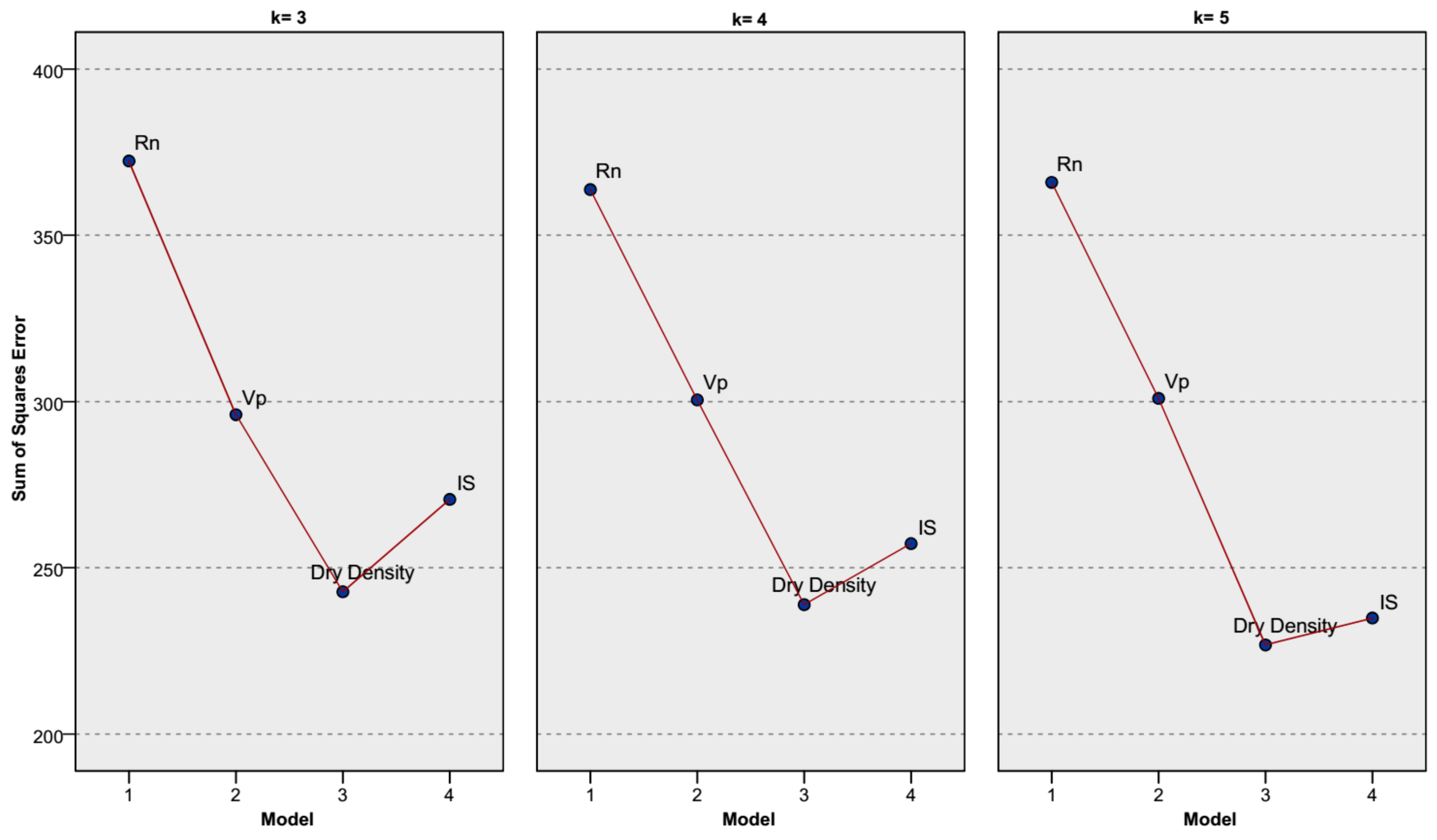
3.1. Evaluation of the Developed Models
3.2. Conqueror Models
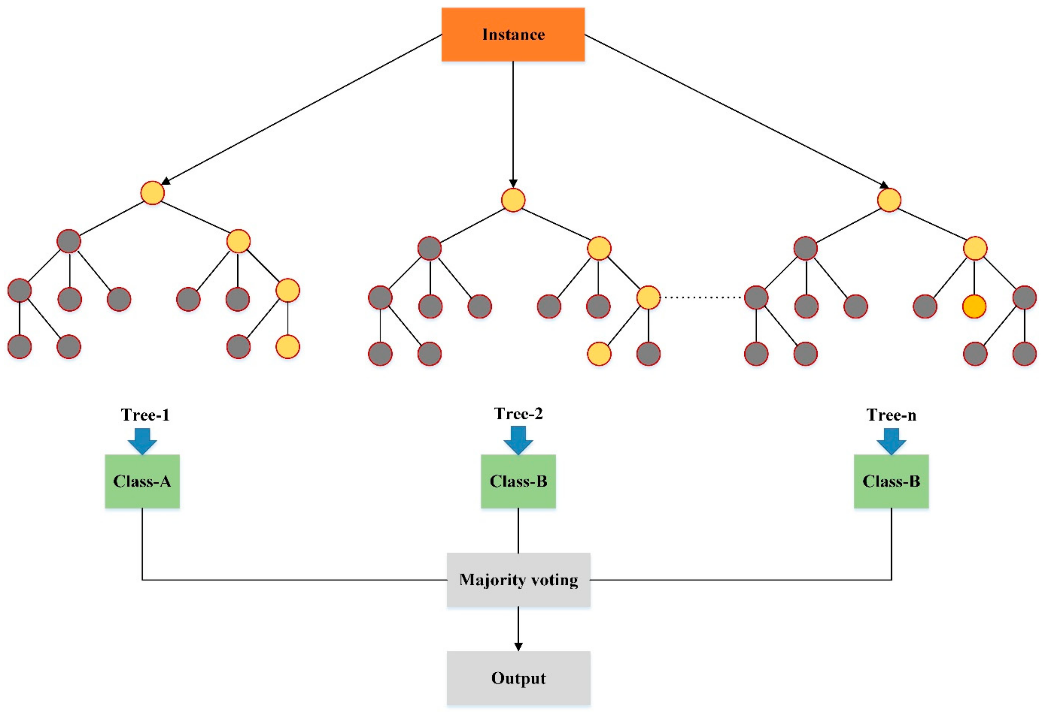
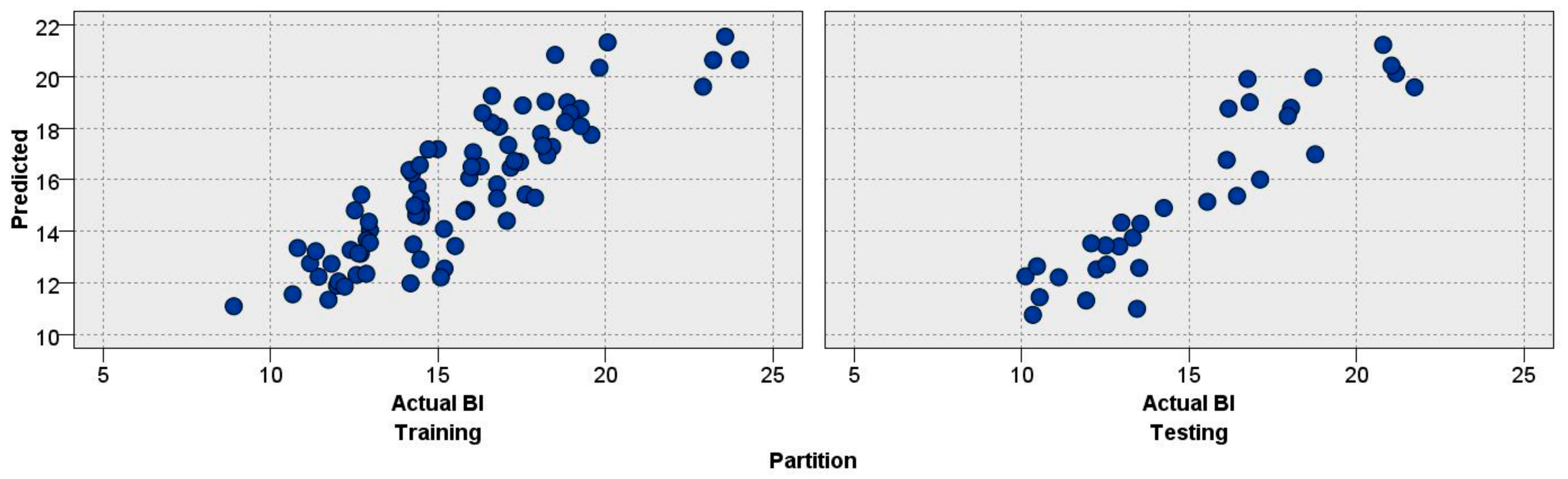
3.2.1. Random Forest Model
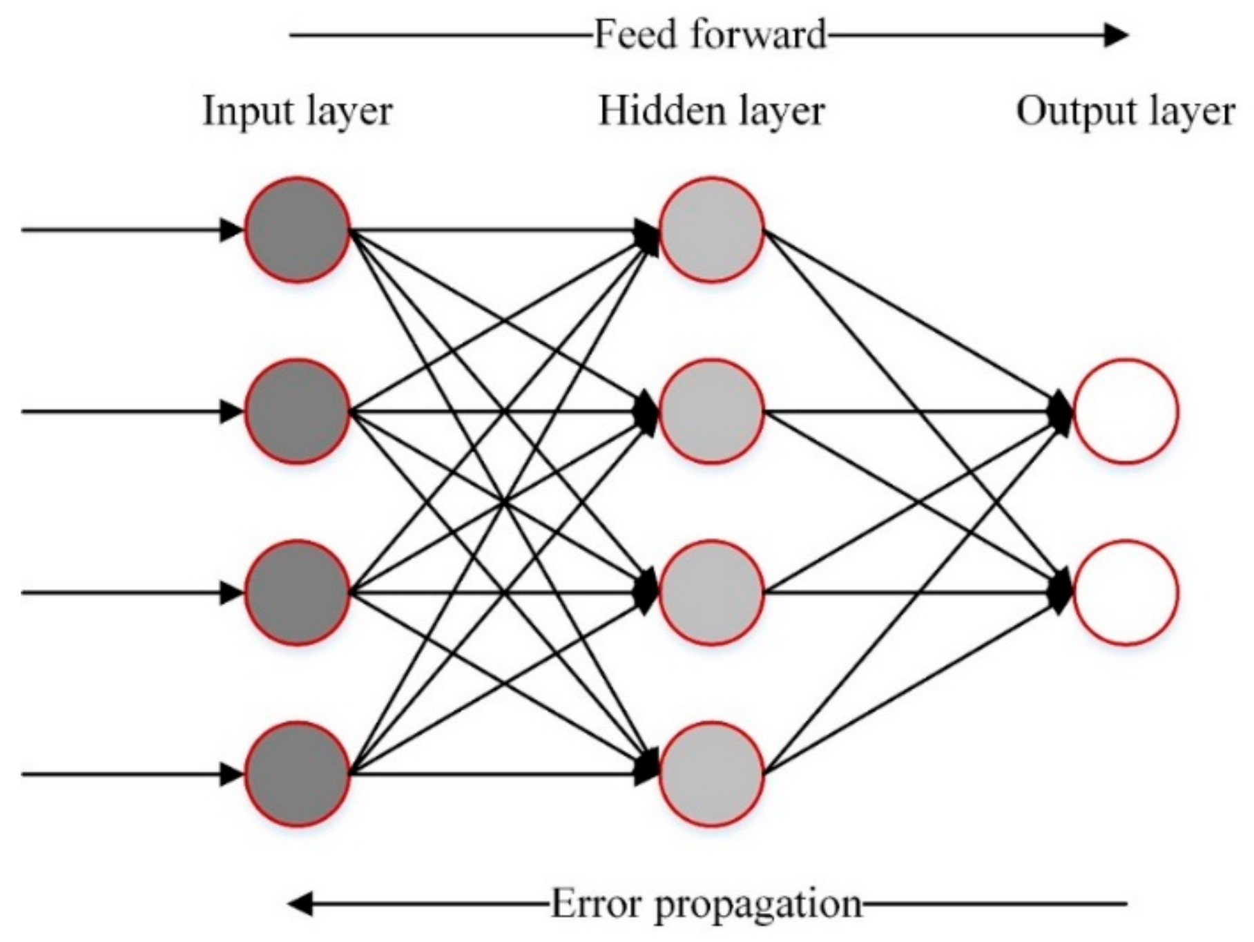
3.2.2. ANN Model
3.2.3. KNN Model
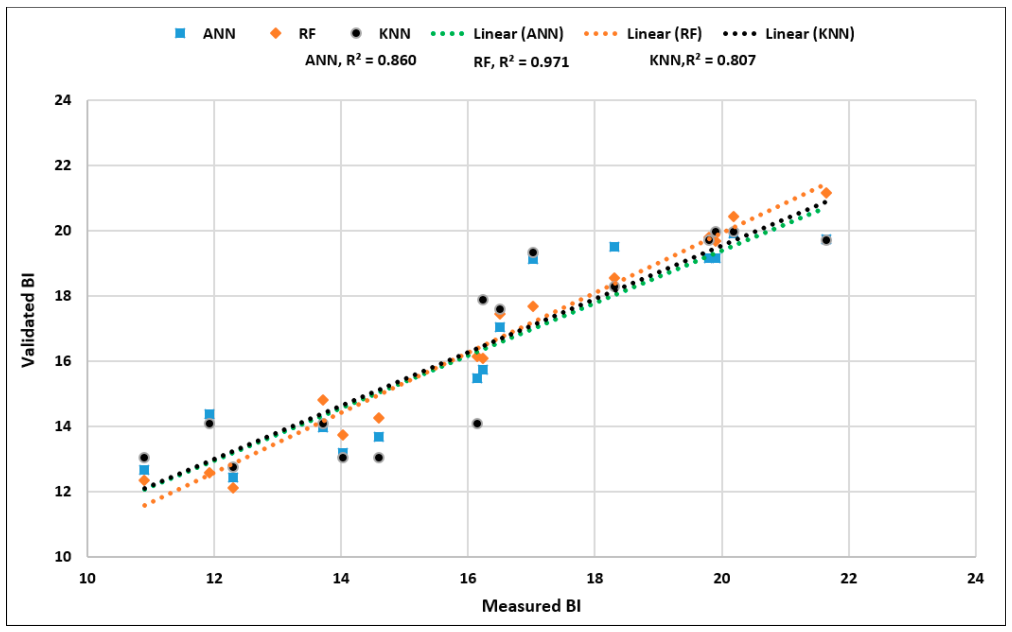
4. Validation of the Selected Models
5. Discussion and Conclusions
Author Contributions
Acknowledgments
Conflicts of Interest
References
- Miskimins, J.L. The impact of mechanical stratigraphy on hydraulic fracture growth and design considerations for horizontal wells. Bulletin 2012, 91, 475–499. [Google Scholar]
- Rybacki, E.; Reinicke, A.; Meier, T.; Makasi, M.; Dresen, G. What controls the mechanical properties of shale rocks?–Part I: Strength and Young’s modulus. J. Pet. Sci. Eng. 2015, 135, 702–722. [Google Scholar] [CrossRef]
- Hajiabdolmajid, V.; Kaiser, P. Brittleness of rock and stability assessment in hard rock tunneling. Tunn. Undergr. Space Technol. 2003, 18, 35–48. [Google Scholar] [CrossRef]
- Kidybiński, A. Bursting liability indices of coal. Int. J. Rock Mech. Min. Sci. Geomech. Abstr. 1981, 18, 295–304. [Google Scholar] [CrossRef]
- Singh, S.P. Brittleness and the mechanical winning of coal. Min. Sci. Technol. 1986, 3, 173–180. [Google Scholar] [CrossRef]
- Singh, S.P. Burst energy release index. Rock Mech. Rock Eng. 1988, 21, 149–155. [Google Scholar] [CrossRef]
- Yagiz, S. Utilizing rock mass properties for predicting TBM performance in hard rock condition. Tunn. Undergr. Space Technol. 2008, 23, 326–339. [Google Scholar] [CrossRef]
- Yagiz, S.; Gokceoglu, C. Application of fuzzy inference system and nonlinear regression models for predicting rock brittleness. Expert Syst. Appl. 2010, 37, 2265–2272. [Google Scholar] [CrossRef]
- Altindag, R. Reply to the Discussion by Yagiz on “Assessment of Some Brittleness Indexes in Rock-Drilling Efficiency” by Altindag. Rock Mech. Rock Eng. 2010, 43, 375–376. [Google Scholar] [CrossRef]
- Yagiz, S. Assessment of brittleness using rock strength and density with punch penetration test. Tunn. Undergr. Space Technol. 2009, 24, 66–74. [Google Scholar] [CrossRef]
- Morley, A. Strength of Material; Longmans: Suffolk, UK, 1944. [Google Scholar]
- Ramsay, J.G. Folding and fracturing of rocks. McGraw Hill B Co. 1967, 568, 289. [Google Scholar]
- Obert, L.; Duvall, W.I. Rock Mechanics and the Design of Structures in Rock; John Wiley & Sons Inc.: Hoboken, NJ, USA, 1967; Volume 278. [Google Scholar]
- Altindag, R.; Guney, A. Predicting the relationships between brittleness and mechanical properties (UCS, TS and SH) of rocks. Sci. Res. Essays 2010, 5, 2107–2118. [Google Scholar]
- Wang, Y.; Watson, R.; Rostami, J.; Wang, J.Y.; Limbruner, M.; He, Z. Study of borehole stability of Marcellus shale wells in longwall mining areas. J. Pet. Explor. Prod. Technol. 2014, 4, 59–71. [Google Scholar] [CrossRef]
- Koopialipoor, M.; Noorbakhsh, A.; Noroozi Ghaleini, E.; Jahed Armaghani, D.; Yagiz, S. A new approach for estimation of rock brittleness based on non-destructive tests. Nondestruct. Test. Eval. 2019, 1–22. [Google Scholar] [CrossRef]
- Khandelwal, M.; Faradonbeh, R.S.; Monjezi, M.; Armaghani, D.J.; Majid, M.Z.B.A.; Yagiz, S. Function development for appraising brittleness of intact rocks using genetic programming and non-linear multiple regression models. Eng. Comput. 2017, 33, 13–21. [Google Scholar] [CrossRef]
- Nejati, H.R.; Moosavi, S.A. A new brittleness index for estimation of rock fracture toughness. J. Min. Environ. 2017, 8, 83–91. [Google Scholar]
- Hajihassani, M.; Abdullah, S.S.; Asteris, P.G.; Armaghani, D.J. A Gene Expression Programming Model for Predicting Tunnel Convergence. Appl. Sci. 2019, 9, 4650. [Google Scholar] [CrossRef]
- Asteris, P.G.; Armaghani, D.J.; Hatzigeorgiou, G.D.; Karayannis, C.G.; Pilakoutas, K. Predicting the shear strength of reinforced concrete beams using Artificial Neural Networks. Comput. Concr. 2019, 24, 469–488. [Google Scholar]
- Zhou, J.; Bejarbaneh, B.Y.; Armaghani, D.J.; Tahir, M.M. Forecasting of TBM advance rate in hard rock condition based on artificial neural network and genetic programming techniques. Bull. Eng. Geol. Environ. 2019. [Google Scholar] [CrossRef]
- Yong, W.; Zhou, J.; Armaghani, D.J.; Tahir, M.M.; Tarinejad, R.; Pham, B.T.; Van Huynh, V. A new hybrid simulated annealing-based genetic programming technique to predict the ultimate bearing capacity of piles. Eng. Comput. 2020. [Google Scholar] [CrossRef]
- Zhou, J.; Guo, H.; Koopialipoor, M.; Armaghani, D.J.; Tahir, M.M. Investigating the effective parameters on the risk levels of rockburst phenomena by developing a hybrid heuristic algorithm. Eng. Comput. 2020. [Google Scholar] [CrossRef]
- Mahdiyar, A.; Jahed Armaghani, D.; Koopialipoor, M.; Hedayat, A.; Abdullah, A.; Yahya, K. Practical Risk Assessment of Ground Vibrations Resulting from Blasting, Using Gene Expression Programming and Monte Carlo Simulation Techniques. Appl. Sci. 2020, 10, 472. [Google Scholar] [CrossRef]
- Zhou, J.; Li, X.; Mitri, H.S. Evaluation method of rockburst: State-of-the-art literature review. Tunn. Undergr. Space Technol. 2018, 81, 632–659. [Google Scholar] [CrossRef]
- Zhou, J.; Li, E.; Yang, S.; Wang, M.; Shi, X.; Yao, S.; Mitri, H.S. Slope stability prediction for circular mode failure using gradient boosting machine approach based on an updated database of case histories. Saf. Sci. 2019, 118, 505–518. [Google Scholar] [CrossRef]
- Zhou, J.; Shi, X.; Li, X. Utilizing gradient boosted machine for the prediction of damage to residential structures owing to blasting vibrations of open pit mining. J. Vib. Control 2016, 22, 3986–3997. [Google Scholar] [CrossRef]
- Zhou, J.; Li, X.; Mitri, H.S. Comparative performance of six supervised learning methods for the development of models of hard rock pillar stability prediction. Nat. Hazards 2015, 79, 291–316. [Google Scholar] [CrossRef]
- Yang, H.; Liu, J.; Liu, B. Investigation on the cracking character of jointed rock mass beneath TBM disc cutter. Rock Mech. Rock Eng. 2018, 51, 1263–1277. [Google Scholar] [CrossRef]
- Yang, H.Q.; Li, Z.; Jie, T.Q.; Zhang, Z.Q. Effects of joints on the cutting behavior of disc cutter running on the jointed rock mass. Tunn. Undergr. Space Technol. 2018, 81, 112–120. [Google Scholar] [CrossRef]
- Chen, H.; Asteris, P.G.; Jahed Armaghani, D.; Gordan, B.; Pham, B.T. Assessing Dynamic Conditions of the Retaining Wall: Developing Two Hybrid Intelligent Models. Appl. Sci. 2019, 9, 1042. [Google Scholar] [CrossRef]
- Liu, B.; Yang, H.; Karekal, S. Effect of Water Content on Argillization of Mudstone during the Tunnelling process. Rock Mech. Rock Eng. 2019. [Google Scholar] [CrossRef]
- Armaghani, D.J.; Hatzigeorgiou, G.D.; Karamani, C.; Skentou, A.; Zoumpoulaki, I.; Asteris, P.G. Soft computing-based techniques for concrete beams shear strength. Procedia Struct. Integr. 2019, 17, 924–933. [Google Scholar] [CrossRef]
- Apostolopoulou, M.; Armaghani, D.J.; Bakolas, A.; Douvika, M.G.; Moropoulou, A.; Asteris, P.G. Compressive strength of natural hydraulic lime mortars using soft computing techniques. Procedia Struct. Integr. 2019, 17, 914–923. [Google Scholar] [CrossRef]
- Xu, H.; Zhou, J.G.; Asteris, P.; Jahed Armaghani, D.; Tahir, M.M. Supervised Machine Learning Techniques to the Prediction of Tunnel Boring Machine Penetration Rate. Appl. Sci. 2019, 9, 3715. [Google Scholar] [CrossRef]
- Huang, L.; Asteris, P.G.; Koopialipoor, M.; Armaghani, D.J.; Tahir, M.M. Invasive Weed Optimization Technique-Based ANN to the Prediction of Rock Tensile Strength. Appl. Sci. 2019, 9, 5372. [Google Scholar] [CrossRef]
- Asteris, P.G.; Mokos, V.G. Concrete compressive strength using artificial neural networks. Neural Comput. Appl. 2019. [Google Scholar] [CrossRef]
- Asteris, P.G.; Nikoo, M. Artificial bee colony-based neural network for the prediction of the fundamental period of infilled frame structures. Neural Comput. Appl. 2019. [Google Scholar] [CrossRef]
- Asteris, P.G.; Moropoulou, A.; Skentou, A.D.; Apostolopoulou, M.; Mohebkhah, A.; Cavaleri, L.; Rodrigues, H.; Varum, H. Stochastic Vulnerability Assessment of Masonry Structures: Concepts, Modeling and Restoration Aspects. Appl. Sci. 2019, 9, 243. [Google Scholar] [CrossRef]
- Kaunda, R.B.; Asbury, B. Prediction of rock brittleness using nondestructive methods for hard rock tunneling. J. Rock Mech. Geotech. Eng. 2016, 8, 533–540. [Google Scholar] [CrossRef]
- Kass, G.V. An exploratory technique for investigating large quantities of categorical data. J. R. Stat. Soc. Ser. C Appl. Stat. 1980, 29, 119–127. [Google Scholar] [CrossRef]
- Brown, G. Ensemble Learning. In Encyclopedia of Machine Learning; Springer: Boston, MA, USA, 2010; pp. 312–320. [Google Scholar]
- Breiman, L. Random forests. Mach. Learn. 2001, 45, 5–32. [Google Scholar] [CrossRef]
- Wu, X.; Kumar, V.; Quinlan, J.R.; Ghosh, J.; Yang, Q.; Motoda, H.; McLachlan, G.J.; Ng, A.; Liu, B.; Philip, S.Y. Top 10 algorithms in data mining. Knowl. Inf. Syst. 2008, 14, 1–37. [Google Scholar] [CrossRef]
- Akbulut, Y.; Sengur, A.; Guo, Y.; Smarandache, F. NS-k-NN: Neutrosophic set-based k-nearest neighbors classifier. Symmetry 2017, 9, 179. [Google Scholar] [CrossRef]
- Qian, Y.; Zhou, W.; Yan, J.; Li, W.; Han, L. Comparing machine learning classifiers for object-based land cover classification using very high resolution imagery. Remote Sens. 2015, 7, 153–168. [Google Scholar] [CrossRef]
- Kavzoglu, T.; Sahin, E.K.; Colkesen, I. Landslide susceptibility mapping using GIS-based multi-criteria decision analysis, support vector machines, and logistic regression. Landslides 2014, 11, 425–439. [Google Scholar] [CrossRef]
- Hasanipanah, M.; Monjezi, M.; Shahnazar, A.; Armaghani, D.J.; Farazmand, A. Feasibility of indirect determination of blast induced ground vibration based on support vector machine. Measurement 2015, 75, 289–297. [Google Scholar] [CrossRef]
- Kalantar, B.; Pradhan, B.; Naghibi, S.A.; Motevalli, A.; Mansor, S. Assessment of the effects of training data selection on the landslide susceptibility mapping: A comparison between support vector machine (SVM), logistic regression (LR) and artificial neural networks (ANN). Geomat. Nat. Hazards Risk 2018, 9, 49–69. [Google Scholar] [CrossRef]
- Cortes, C.; Vapnik, V. Support-vector networks. Mach. Learn. 1995, 20, 273–297. [Google Scholar] [CrossRef]
- Hong, H.; Pradhan, B.; Bui, D.T.; Xu, C.; Youssef, A.M.; Chen, W. Comparison of four kernel functions used in support vector machines for landslide susceptibility mapping: A case study at Suichuan area (China). Geomat. Nat. Hazards Risk 2017, 8, 544–569. [Google Scholar] [CrossRef]
- Kamavisdar, P.; Saluja, S.; Agrawal, S. A survey on image classification approaches and techniques. Int. J. Adv. Res. Comput. Commun. Eng. 2013, 2, 1005–1009. [Google Scholar]
- Liu, J.; Savenije, H.H.G.; Xu, J. Forecast of water demand in Weinan City in China using WDF-ANN model. Phys. Chem. Earth Parts A/B/C 2003, 28, 219–224. [Google Scholar] [CrossRef]
- Mohamad, E.T.; Armaghani, D.J.; Noorani, S.A.; Saad, R.; Alvi, S.V.; Abad, N.K. Prediction of flyrock in boulder blasting using artificial neural network. Electron. J. Geotech. Eng. 2012, 17, 2585–2595. [Google Scholar]
- Tonnizam Mohamad, E.; Hajihassani, M.; Jahed Armaghani, D.; Marto, A. Simulation of blasting-induced air overpressure by means of Artificial Neural Networks. Int. Rev. Model. Simul. 2012, 5, 2501–2506. [Google Scholar]
- Asteris, P.; Roussis, P.; Douvika, M. Feed-forward neural network prediction of the mechanical properties of sandcrete materials. Sensors 2017, 17, 1344. [Google Scholar] [CrossRef] [PubMed]
- Apostolopoulour, M.; Douvika, M.G.; Kanellopoulos, I.N.; Moropoulou, A.; Asteris, P.G. Prediction of Compressive Strength of Mortars using Artificial Neural Networks. In Proceedings of the 1st International Conference TMM_CH, Transdisciplinary Multispectral Modelling and Cooperation for the Preservation of Cultural Heritage, Athens, Greece, 10–13 October 2018; pp. 10–13. [Google Scholar]
- Asteris, P.G.; Argyropoulos, I.; Cavaleri, L.; Rodrigues, H.; Varum, H.; Thomas, J.; Lourenço, P.B. Masonry compressive strength prediction using artificial neural networks. In International Conference on Transdisciplinary Multispectral Modeling and Cooperation for the Preservation of Cultural Heritage; Springer: Cham, Germany, 2018; pp. 200–224. [Google Scholar]
- Armaghani, D.J.; Mohamad, E.T.; Narayanasamy, M.S.; Narita, N.; Yagiz, S. Development of hybrid intelligent models for predicting TBM penetration rate in hard rock condition. Tunn. Undergr. Space Technol. 2017, 63, 29–43. [Google Scholar] [CrossRef]
- Momeni, E.; Nazir, R.; Armaghani, D.J.; Maizir, H. Application of artificial neural network for predicting shaft and tip resistances of concrete piles. Earth Sci. Res. J. 2015, 19, 85–93. [Google Scholar] [CrossRef]
- Ulusay, R.; Hudson, J.A. ISRM (2007) The Complete ISRM Suggested Methods for Rock Characterization, Testing and Monitoring: 1974–2006; International Society for Rock Mechanics, Commission on Testing Methods: Ankara, Turkey, 2007; p. 628. [Google Scholar]
- Hucka, V.; Das, B. Brittleness determination of rocks by different methods. Int. J. Rock Mech. Min. Sci. Geomech. Abstr. 1974, 11, 389–392. [Google Scholar] [CrossRef]
- Salaria, S.; Drozd, A.; Podobas, A.; Matsuoka, S. Predicting performance using collaborative filtering. In Proceedings of the 2018 IEEE International Conference on Cluster Computing (CLUSTER), Belfast, UK, 10–13 September 2018; pp. 504–514. [Google Scholar]
- Su, G.S.; Zhang, X.F.; Yan, L.B. Rockburst prediction method based on case reasoning pattern recognition. J. Min. Saf. Eng. 2008, 1, 15. [Google Scholar]


| Parameter | Symbol | Unit | Category | Min | Max | Mean |
|---|---|---|---|---|---|---|
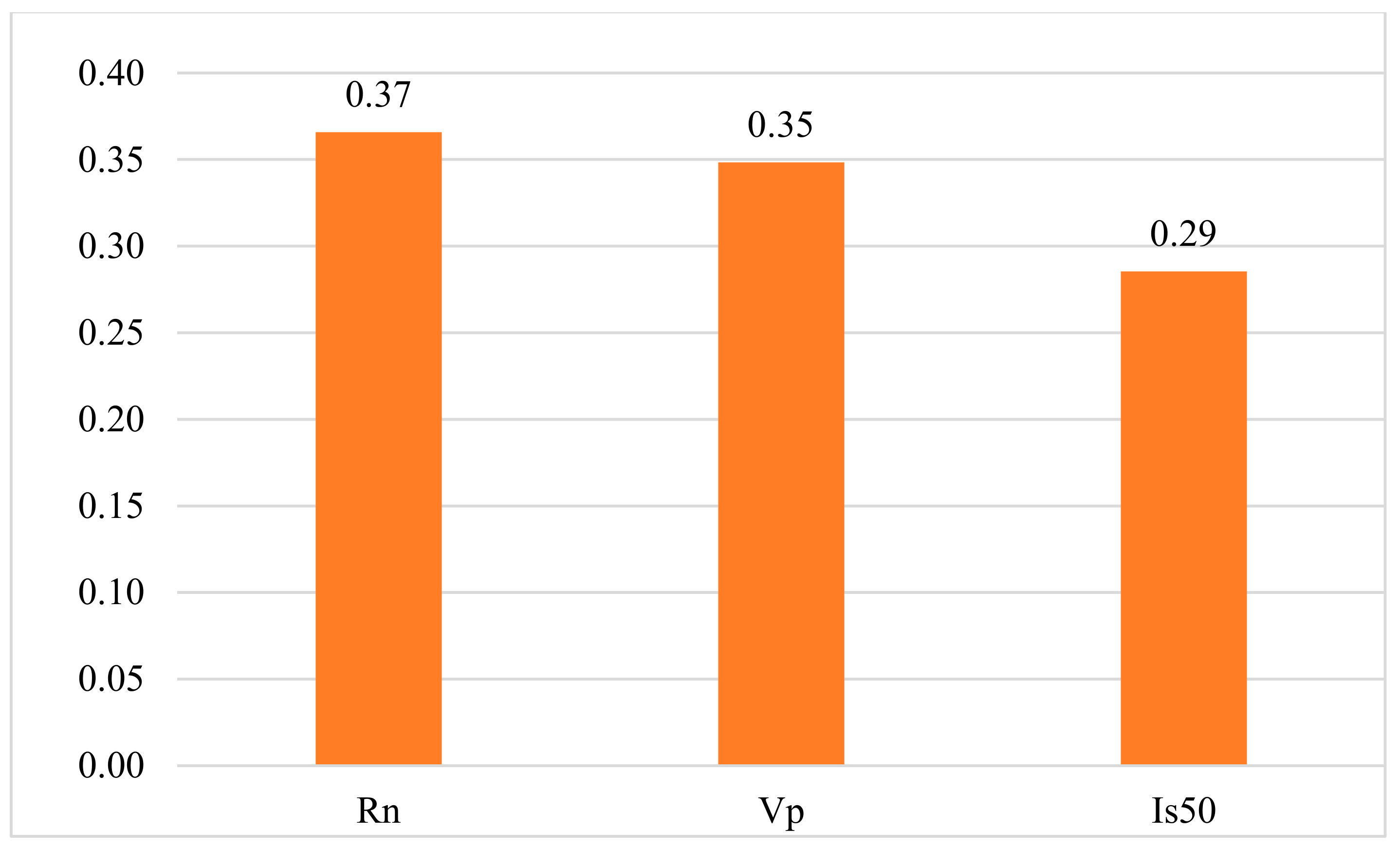
| P-wave velocity | Vp | m/s | Input | 2870 | 7702 | 5491.6 |
| Density | D | g/cm3 | Input | 2.37 | 2.79 | 2.59 |
| Schmidt hammer rebound number | Rn | - | Input | 20 | 61 | 40.5 |
| Point load strength | Is50 | MPa | Input | 0.89 | 7.1 | 3.6 |
| Brittleness index | BI | - | Output | 8.90 | 24.01 | 15.5 |
| Performance Index | RF | CHAID | KNN | SVM | ANN | |||||||||||||||
|---|---|---|---|---|---|---|---|---|---|---|---|---|---|---|---|---|---|---|---|---|
| TR | TE | TR | TE | TR | TE | TR | TE | TR | TE | |||||||||||
| Value | Rank | Value | Rank | Value | Rank | Value | Rank | Value | Rank | Value | Rank | Value | Rank | Value | Rank | Value | Rank | Value | Rank | |
| R2 | 0.89 | 5 | 0.75 | 2 | 0.77 | 3 | 0.74 | 1 | 0.81 | 4 | 0.84 | 4 | 0.73 | 1 | 0.84 | 3 | 0.75 | 2 | 0.85 | 5 |
| RMSE | 1.08 | 5 | 1.75 | 2 | 1.39 | 3 | 1.8 | 1 | 1.33 | 4 | 1.44 | 3 | 1.57 | 1 | 1.42 | 4 | 1.50 | 2 | 1.39 | 5 |
| VAF (%) | 86.84 | 5 | 80.5 | 2 | 78.31 | 3 | 75.1 | 1 | 80.62 | 4 | 86.1 | 3 | 72.62 | 1 | 87.5 | 5 | 74.60 | 2 | 87 | 4 |
| MAE | 0.91 | 5 | 1.36 | 1 | 1.14 | 4 | 1.35 | 2 | 1.16 | 3 | 1.15 | 4 | 1.32 | 1 | 1.06 | 5 | 1.29 | 2 | 1.16 | 3 |
| a20-index | 1.00 | 5 | 0.91 | 2 | 0.95 | 2 | 0.84 | 1 | 0.99 | 4 | 0.97 | 4 | 0.91 | 1 | 0.96 | 3 | 0.97 | 3 | 0.97 | 5 |
| Sum of the ranks | TR | 25 | TE | 9 | TR | 15 | TE | 6 | TR | 19 | TE | 18 | TR | 5 | TE | 20 | TR | 11 | TE | 22 |
| Final rank | 34 | 21 | 37 | 25 | 33 | |||||||||||||||
| Performance Index | RF | ANN | KNN |
|---|---|---|---|
| R2 | 0.971 | 0.860 | 0.807 |
| RMSE | 0.62 | 1.22 | 1.42 |
| VAF (%) | 96.852 | 85.633 | 80.64 |
| MAE | 0.46 | 0.99 | 1.14 |
| a20-index | 1.00 | 1.00 | 1.00 |
© 2020 by the authors. Licensee MDPI, Basel, Switzerland. This article is an open access article distributed under the terms and conditions of the Creative Commons Attribution (CC BY) license (http://creativecommons.org/licenses/by/4.0/).
Share and Cite
Sun, D.; Lonbani, M.; Askarian, B.; Jahed Armaghani, D.; Tarinejad, R.; Thai Pham, B.; Huynh, V.V. Investigating the Applications of Machine Learning Techniques to Predict the Rock Brittleness Index. Appl. Sci. 2020, 10, 1691. https://doi.org/10.3390/app10051691
Sun D, Lonbani M, Askarian B, Jahed Armaghani D, Tarinejad R, Thai Pham B, Huynh VV. Investigating the Applications of Machine Learning Techniques to Predict the Rock Brittleness Index. Applied Sciences. 2020; 10(5):1691. https://doi.org/10.3390/app10051691
Chicago/Turabian StyleSun, Deliang, Mahshid Lonbani, Behnam Askarian, Danial Jahed Armaghani, Reza Tarinejad, Binh Thai Pham, and Van Van Huynh. 2020. "Investigating the Applications of Machine Learning Techniques to Predict the Rock Brittleness Index" Applied Sciences 10, no. 5: 1691. https://doi.org/10.3390/app10051691
APA StyleSun, D., Lonbani, M., Askarian, B., Jahed Armaghani, D., Tarinejad, R., Thai Pham, B., & Huynh, V. V. (2020). Investigating the Applications of Machine Learning Techniques to Predict the Rock Brittleness Index. Applied Sciences, 10(5), 1691. https://doi.org/10.3390/app10051691