Article

Eliminating the Effect of Uncertainties of Cutting Forces by Fuzzy Controller for Robots in Milling Process

1
School of Mechanical Engineering, Hanoi University of Science and Technology, 01 Dai Co Viet, Hai Ba Trung, Hanoi 100000, Vietnam
2
College of Urban Works Construction, Yen Thuong, Gia Lam, Ha Noi 100000, Vietnam
*
Author to whom correspondence should be addressed.
Appl. Sci. 2020, 10(5), 1685; https://doi.org/10.3390/app10051685
Submission received: 8 January 2020 / Revised: 18 February 2020 / Accepted: 26 February 2020 / Published: 2 March 2020
(This article belongs to the Section Mechanical Engineering)

Abstract

:
This study presents a method of controlling robots based on fuzzy logic to eliminate the effect of uncertainties that are generated by the cutting forces in milling process. The common method to control industrial robots is based on the robot dynamic model and the differential equations of motion to compute the control values. The quantities in the differential equations of the motion of robots are complex and difficult to determine fully and accurately. The interaction forces between the cutting tool and the workpiece are the cutting forces, which are generated during the machining process. It is difficult to calculate the cutting force because it depends on many factors such as material of the machining part, depth of cut, feed rate, etc. This article presents the fuzzy rule system and the selection of the physical value domain of input and output variables of the fuzzy controller. The fuzzy rules are applied in this article to allow us to compute the driving forces based on the errors of input and output signals of the joint positions and velocities, thereby avoiding the calculation of cutting forces. This article shows the simulation results of the fuzzy controller and comparison with the results of the conventional controller when the dynamic model is assumed to be correctly determined. The achieved results are reliable and facilitate the research and application of a fuzzy controller to mechanical processing robots in general and milling machining in particular.

1. Introduction

Robots are increasingly being used in mechanical machining due to many technical and economic advantages [1,2,3,4,5]. Robots have many degrees of freedom and a structure with many links and joints enabling them to move flexibly in a large workspace. They have machine parts with complex geometric surfaces, large dimensions, and a minimum number of machining operations and simple jigs [3]. Machining by industrial robots is more economical than machine tools and according to the calculation of the COMET, the price advantage is up to 30% [6]. However, there are many difficulties and challenges in exploiting the potential of robot applications [2,7]. The structure with many links and joints will give the robot the ability to manipulate flexibly as mentioned, but it is difficult when modeling kinematics and dynamics to control the robots. The expressions of the kinematic and dynamic quantities in the differential equations of motion of the robots are often cumbersome and complex. The machining process has many factors, which are difficult to fully and accurately determine, for example, chatter, vibration, or the fact that the perturbations may appear abnormally [8,9,10]. In particular, the cutting force generated during machining is an uncertain factor and has a great effect on the determination of control force based on the dynamic model [11,12,13,14,15,16,17,18,19,20,21,22,23,24,25,26,27,28,29,30,31,32]. The mechanical machining processes often require high accuracy, especially when milling to shape complex surfaces, which requires even more rigorous accuracy of shaping motion. In order to solve these problems, there have been many study directions to improve and enhance the machining accuracy of robots. One of the solutions is controlling based on fuzzy logic to overcome the difficulty of determining cutting forces while ensuring control accuracy. Fuzzy logic is an effective tool for solving many technical problems in general [33,34,35,36,37,38,39,40,41,42,43], in mechanical processing and in industrial robot applications in particular.
There have been many studies on the effect of cutting forces based on fuzzy logic [44,45,46,47]. In addition, there are also many studies on robot control based on fuzzy logic [48,49,50,51,52,53,54,55,56,57,58,59,60,61]. However, the application of fuzzy logic to control robots to eliminate the effect of cutting forces is still an open problem [62,63,64,65,66,67].
The paper proposes a fuzzy law system for a controller to calculate and determine the control forces (driving forces/torques of the motors) based on errors between input and output signals on the joint positions and velocities. The computations based on the control law are simple linear algebra calculations that are easier and faster to perform than calculating the generalized force expression of cutting forces in the differential equations of motion of robots.
It is assumed that the dynamic model of robots is precisely determined, including the cutting forces in the differential equations of motion, which is considered to be accurately determined. This article presents the application of a common (conventional and popular) method in controlling industrial robots, meaning the inverse dynamics method combined with the law of derivative proportional control (PD), hereinafter referred to as the Inverse Dynamics + PD method. With the above assumption, the Inverse Dynamics + PD controller is considered an accurate one. To distinguish, the controllers based entirely on the dynamic model are called (hereinafter) explicit (crisp) controllers.
The article shows the results of simulating the fuzzy controller in comparison with the results of simulating the above explicit and accurate controller. With the different assumption of cutting force calculation, that is, choosing the different influenced coefficients in calculating cutting forces, the Inverse Dynamics + PD controller will give different results, meaning that the control errors are significant. With the fuzzy controller, due to the determination of cutting forces not being required, even if the components of the cutting force change, or the occurrence of perturbation, then the controller’s performance will still ensure the accuracy of desired motion laws (desired trajectories).
The remains of this article is organized as follows. Section 2 briefly presents robot kinematic modeling based on the authors of [68,69,70,71,72] to indicate necessary computations for receiving the motion trajectory of robots, which is used for the following studies. Section 3 discusses dynamics modeling, presents the derivation of robot’s dynamic model, and analyzes the calculation of cutting forces with an empirical formula. Section 4 presents a familiar control method that is used as a basis for comparison. Section 5 presents the steps to build the fuzzy controller, and proposes a fuzzy control law that is suitable for a controller of a robot in milling machining. Section 6 presents the results of simulation, calculation and comparative analysis. Section 7 presents the conclusions, analyzing the possibility of applying the proposed controller, and discusses the directions of future studies.

2. Robot Kinematic Modeling

The system of the robot has a clamping platform with eight degrees of freedom (DOF), including a robot and a platform, which allows expanding the machining space (Figure 1). The robot is designed according to the robot model of Asea Brown Boveri, which is a six DOF serial robot, consisting of six moveable links connected to a fixed base. The cutting tool is mounted on the end effector of the robot. The platform has two DOF, including two moveable links; the workpiece is fixed on the upper link. Names of the robot links and platform links of the system in turn are: L0, L1, …, L6, B and D, respectively. Link L0 is the base, link L6 is the end effector, link B connects the prismatic joint to the fixed base, and link D carries the workpiece. The robot and the clamping platform coordinate programmatically to perform the form-shaping motion of the machining surface.
Normally, the machining object is clamped on a fixed platform, and a robot with 6 DOF is sufficient to obtain positions and orientations of the end effector for the machining performance. However, for the purpose of expanding the operational space of the robot, or choosing a convenient machining posture, a machining system with a two DOF clamping platform is utilized. As a result, the robot can machine large parts with many complex surfaces, reducing the number of clamping operations. Robots with a combination of two such component robots or more are often referred to Mechanism of Relative Manipulation robots—MRM [73,74,75,76,77,78,79,80,81]. For a simple presentation, the robot–platform system is hereinafter called the robot system or the robot.
The article applies the Denavit–Hartenberg convention to define the link frames and derive kinematic equations of the robot kinematic chains, using generalized coordinates to represent and calculate the kinematic chain of the platform. The coordinate systems, kinematic parameters and corresponding homogeneous coordinate transformation matrices are shown in Table 1.
In Table 1, Oixiyizi (i = 1, …, 6) is the frame that is attached to the end of link i, and represents the position and orientation of frame Oixiyizi with respect to frame Oi−1xi−1yi−1zi−1 by the Denavit–Hartenberg homogeneous coordinate transformation matrix i−1Ai, with respect to frame O0x0y0z0 by matrix 0Ai. O6x6y6z6 is called the end-effector frame. O0x0y0z0 is called the base frame for the entire robot–platform system, with matrix E being the 4 × 4 identity matrix that represents the position and orientation of the base frame with respect to itself. The parameters in the third column of Table 1 represent the relative positions between two consecutive frames, in which θi (i = 1, …, 6), yb, xd are the joint coordinates, and the other parameters are constants.
The vector of joint coordinate is denoted by q, represented by Equation (1).
q = [ q 1 , , q 8 ] T = [ θ 1 , , θ 6 , y b , x d ] T
O0’x0’y0’z0’ is the fixed frame that has the origin at position O0’ and the axes parallel to the corresponding ones of the base frame, used to location the platform.
Obxbybzb is the frame that attached to link B; it is possible to translate in the direction yb//y0, corresponding to the joint coordinate yb, the coordinate transformation matrices as shown in Table 1. Odxdydzd is the frame that attached to link D; it is possible to translate in the direction xd//xb//x0, corresponding to the joint coordinate xd, the coordinate transformation matrices as shown in Table 1.
Frame Odxdydzd, hereinafter called the platform frame or the jig frame, is used to locate the workpiece. The parameters of the workpiece’s machined surface and toolpath are shown in the jig frame.
In the machining process, the tool performs the relative motion with respect to the machined surface according to the law (trajectory) that is determined by the machining engineering. This trajectory is represented by parameters dxE, dyE, dzE, dαE, dβE, dηE (Table 1) and their first and second time derivatives with respect to time. Thereby, the vector of operational coordinates is called p, represented by (2).
p = p d E = [ p d 1 , p d 2 , , p d 6 ] T = [ x d E , y d E , z d E , α d E , β d E , η d E ] T
Therefore, the frame Odxdydzd is used as the operational frame.
Frame OExEyEzE is attached to the cutting edge of the cutter on the end effector, called the tool frame.
According to the robot kinematic chain, matrix 0AE represents the position and orientation of the tool frame OExEyEzE with respect to the base frame O0x0y0z0, determined by (3).
A 0 E = A 0 1 ( θ 1 ) A 1 2 ( θ 2 ) A 5 6 ( θ 6 ) A 6 E
According to the platform kinematic chain, 0AE is determined by (4).
A 0 E = A 0 0 A 0 b ( y b ) A b d ( x d ) A d E ( p )
From (3) and (4), we obtained (5).
A d E ( p ) = A b d 1 ( x d ) A 0 b 1 ( y b ) A 0 0 1 0 A 1 ( θ 1 ) 5 A 6 ( θ 6 ) A 6 E
The right hand side of (5) is the matrix representing the position and orientation of the cutting tool with respect to the platform frame Odxdydzd, whose elements are functions of the joint coordinates (1). Meanwhile, the elements of the matrix on the left hand side of (5) are functions of the operational coordinates (2). (5) is rewritten by (6).
[ C d p ( α d E , β d E , η d E ) r d E ( x d E , y d E , z d E ) 0 T 1 ] = [ C d E ( q ) r d E ( q ) 0 T 1 ]
Equation (6) is called the kinematic equation of robot in matrix form.
For each specific machining case, the requirements on shaping motion of the tool are given. That is, to the scope of this study, the operational coordinates (2) and its derivatives are known. Applying the accompanying trihedron method [68,69,70,71,72] together with the kinematic Equation (6) allows us to calculate the motion trajectory of the robot. That is, the joint coordinates (1) and their first and second time derivatives with respect to time are calculated, which are used as the set trajectories (7) for the control problem in the following section.
{ q d = [ θ 1 , θ 2 , , θ 6 , y b , x d ] T = [ q 1 d , , q 8 d ] T q ˙ d = [ θ ˙ 1 , θ ˙ 2 , , θ ˙ 6 , y ˙ b , x ˙ d ] T = [ q ˙ 1 d , , q ˙ 8 d ] T q ¨ d = [ θ ¨ 1 , θ ¨ 2 , , θ ¨ 6 , y ¨ b , x ¨ d ] T = [ q ¨ 1 d , , q ¨ 8 d ] T

3. Robot Dynamic Modeling

3.1. Differential Equations of Motion of the Robot

The Lagrange equation in matrix form describing the motion of the robot has form (8).
[ M ( q ) ] ( 8 × 8 ) q ¨ ( 8 × 1 ) + [ C ( q , q ˙ ) q ˙ ] ( 8 × 1 ) + [ G ( q ) ] ( 8 × 1 ) + [ Q ] ( 8 × 1 ) = [ U ] ( 8 × 1 )
In which [M(q)]8×8 is the mass matrix of the robot system, calculated through mass mi, translation Jacobian matrix JTi, rotation Jacobian matrix ciJRi and inertia tensor CiΘCi of link i (9).
[ M ( q ) ] ( 8 × 8 ) = [ i = 1 8 ( J Ti T m i J Ti + J ci Ri T Θ ci ci ci J Ri ) ] ( 8 × 8 )
[ C ( q , q ˙ ) q ˙ ] 8 × 1 is the vector of the generalized forces of Coriolis and centrifugal inertial forces, calculated through the partial derivative of the elements of matrix [M(q)] with respect to the generalized coordinates q, and the generalized velocity q ˙ (10).
[ C ( q , q ˙ ) q ˙ ] ( 8 × 1 ) = [ c 1 , c 2 , , c 8 ] T ;    c j = k , l = 1 8 ( k , l ; j ) q ˙ k q ˙ l ;    ( k , l ; j ) = 1 2 ( m k j q l + m l j q k m k l q j )
(k,l;j) is Christoffel notation with 3 indexes of the first kind; mkl (k,l = 1,…, 8) are the elements of matrix [M(q)].
[G(q)]8×1 is the vector of the generalized forces of the conservative forces (11).
[ G ( q ) ] ( 8 × 1 ) = [ G 1 , G 2 , , G 8 ] T ; G j = Π q j
Π is the potential energy of the system.
[U]8×1 is the vector of the generalized forces of the driving forces/torques (12).
[ U ] ( 8 × 1 ) = [ U 1 , U 2 , , U 8 ] T ; U i = τ i
τi is the driving force at joint i. τi is the force or torque depending on the prismatic joint or revolute joint.
[Q(q)]8×1 is the vector of the generalized forces of the non-conservative forces, including the friction forces at the contact point between the tool and the workpiece, the forces that separate the chip from the workpiece; the acting forces between the tool and the workpiece are called the cutting forces, collectively. In addition, there are also the friction forces at the joints, the abnormal perturbation from the environment, etc., of which the value of cutting forces and the effect of cutting forces on motion are great. Therefore, this paper limits the investigation of cutting forces and other types of force are ignored. The next subsection introduces the investigation of cutting forces in milling process with the robot.

3.2. Cutting Forces in Milling

The cutting forces are generated at the cutting point of the tool and the workpiece and this is a complex process force system. However, in general, the process force system can be represented as the force system from the workpiece acting on the robot including the force and the torque (force couple) with notation (Fc,Mc). The notation (Fr,Mr) represents the force and torque vectors from a tool acting on the workpiece (13).
F c = [ F x , F y , F z ] T ; M c = [ M x , M y , M z ] T ; F r = F c ;   M r = M c
The generalized force components of the force Fc and the torque Mc are determined by the robot kinematic chain (14).
Q c = J TE T F C   + J RE T M c   = [ J TE T , J RE T ] [ F c , M c ] T   = J E T R c
rE is the position vector of the acting point of the force Fc with respect to the base frame, ωE is the angular velocity of the end effector, determined by the robot kinematic chain. The Jacobian matrices in (14) are calculated according to (15).
J TE = r E q ; J RE = ω E q ˙
The generalized force components of the force Fr and the torque Mr are determined according to the platform kinematic chain (16).
Q r = J Tr T F r   + J Rr T M r   = [ J Tr T , J Rr T ] [ F r , M r ] T   = J r T R r
rk is the position vector of acting point of the force Fr with respect to the base frame and ωk is the angular velocity of the workpiece determined by the platform kinematic chain. The Jacobian matrices in (16) are calculated according to (17).
J T r = r k q ; J Rr = ω k q ˙
Note that Equation (17) is used for the general case; with the robot system investigated in this paper, the angular velocity ωk is zero because the platform carrying the workpiece has only two prismatic joints, and only performs translational motion.
It is known that on the robot kinematic chain, there are only joint coordinates q1,q2, …, q6; while on the platform kinematic chain, there are only joint coordinates q7, q8, therefore we have (18) and (19).
Q c = [ Q c 1 , Q c 2 , , Q c 6 , 0 , 0 ] T
Q r = [ 0 , 0 , , 0 , Q r 7 , Q r 8 ] T
So, the sum of the generalized force components of the non-conservative forces is expressed as (20).
[ Q ( q ) ] ( 8 × 1 ) = Q c + Q r = [ Q c 1 , Q c 2 , , Q c 6 , Q r 7 , Q r 8 ] T
Recognizing that in order to calculate the generalized forces of cutting forces, the Jacobian matrices calculated according to (15) are quite complex, because the expressions for determining the position of cutting points and the angular velocity of the end effector are often cumbersome and complex.
The cutting forces expressing as (13) appear in milling process depending on the cutting parameters, the geometric parameters of the chip geometry, cutting conditions, etc. The cutting force components are not constants because the materials are heterogeneous, and the depth of cut, the feed rate, etc., may be changed during the machining process. The cutting forces are complex distribution forces on the contact area between the surface of the cutting edge and the workpiece, with the resultant force placed at the center of the contact area (placed at the upper point of the cutting edge between the cutter entry and exit angles).
According to the authors of [25,26], the approximate method of calculating the milling forces in the x, y, z directions of the Z cutting teeth is represented by (21).
F x = i = 1 z F x , i ; F y = i = 1 z F y , i ; F z = i = 1 z F z , i
where Fx,i, Fy,i, Fz,i are the cutting forces acting on the ith cutting edge in the x, y, z directions, respectively, calculated according to (22).
F f , i ( θ i ( z ) ) = z j , 1 z j , 2 d F f , i ( θ i ( z ) ) dz ;   f   =   x , y , z
In which zj,1i(z)), zj,2i(z)) are upper and lower limitations of the cutting area of the ith cutting edge, in axial direction of the cutter shaft.
d F x i , d F y i , d F z i are the differential cutting forces acting on the infinitesimal cutting edge segment of the ith cutting edge, in x, y, z directions, respectively (23).
[ d F xi d F yi d F zi ] = [ cos θ i sin θ i sin κ sin θ i cos κ sin θ i cos θ i sin κ cos θ i cos κ 0 cos κ sin κ ] [ d F t i d F r i d F a i ]
θ i ( z ) is the immersion angle for the cutting edge i at axial depth of cut z (24):
θ i ( z ) = θ ( t ) + θ p i ψ ( z ) ; i   =   1 ,   ,   Z ; θ ( t ) = 2 π n 60 t ; θ pi = ( 1 i ) 2 π Z
κ is the angle between dFri and the cutter axial; Z is number of cutting edge/flute/tooth of the cutter; Ψ(z) is the radial lag angle; n is spindle speed (rpm).
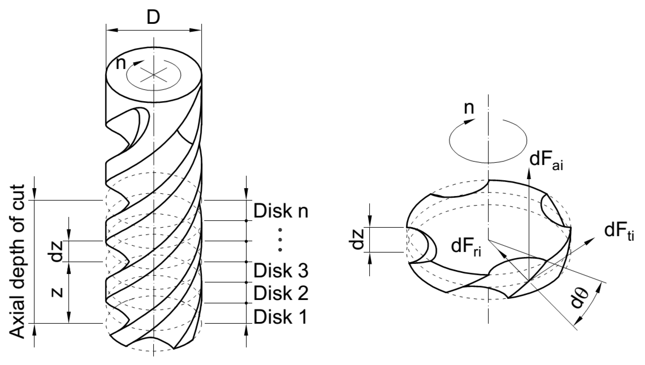
At instant t, at any point P of the cutting area, a segment of the ith cutting edge performs cutting, the differential cutting forces dFti, dFri, dFai in tangential, radial and axial directions, respectively, acting on point P, represented in Figure 2 and determined by (25).
{ d F t i = K t c a i ( θ i , κ ) d b + K d t e S d F r i = K r c a i ( θ i , κ ) d b + K d r e S d F a i = K a c a i ( θ i , κ ) d B + K d a e S
Of which:
Ktc, Krc, Kac are tangential, radial and axial cutting force coefficients in milling.
Kte, Kre, Kae are tangential, radial and axial edge force coefficients in milling.
dS is thickness of an element of the ith cutting edge.
db is length of cut in the direction of the cutting velocity vector.
aii,κ) is chip thickness that cut by the segment of the ith cutting edge (26).
a ( θ i , κ ) = S z sin θ i sin κ
The force components according to (21)–(23) can be conveniently represented on the x, y, z axes of the tool frame OExEyEzE. Summing the cutting force system with respect to the origin of the tool frame, we obtain the torques of the cutting forces. These torques are determined based on the position of the acting point of resultant force of the cutting force system with respect to the tool frame OExEyEzE. The contact area and the state of interaction between the tool and the workpiece are difficult to determine accurately, therefore, the determination of the resultant force value of the cutting force system and their positions, as well as their torques, are complex and less accurate. This study does not aim to find out an accurate calculation of the cutting forces but rather to find out the way to eliminate its effects.
The next section represents the application of a dynamic model that is derived above for the Inverse Dynamics + PD controller.

4. Inverse Dynamics + PD Controller

The control of the 8 DOF robot–platform system is the coordinating movement control of the 6 DOF robot with the tool and the 2 DOF platform with the workpiece so as to ensure the tool tracking on the given form-shaping tool path in the task space. Movement of the robot system is carried out thanks to the joint driving system. The control effects are applied to the joints, so the joints are directly the control objects; the joint positions always follow to the desired positions so that the position deviations (error) are less than a specified value consistent with the required accuracy.
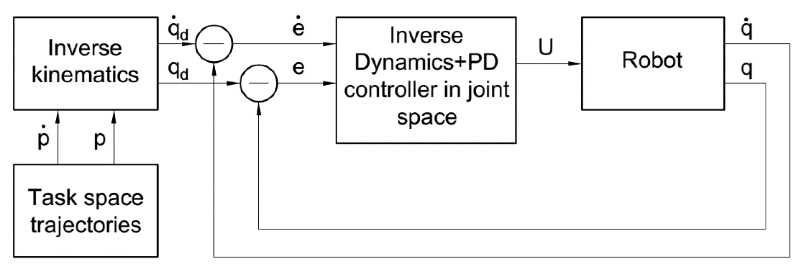
The Inverse Dynamics + PD controller is the common controller, popular for industrial robots, based on the rule of inverse dynamics control combined with the outer loop linear PD control.
Using the differential equations of motion of robot system (8), choosing the control rule as follows (27).
[ U ] = [ U ] ( 8 × 1 ) = [ M ( q ) ] ( 8 × 8 ) u ( 8 × 1 ) + [ C ( q , q ˙ ) q ˙ ] ( 8 × 1 ) + [ G ( q ) ] ( 8 × 1 ) + [ Q ( q ) ] ( 8 × 1 )
u is the chosen control signal that has the PD structure (28).
U = q ¨ d ( 8 × 1 ) + K v ( 8 × 8 ) e ˙ ( 8 × 1 ) + K p ( 8 × 8 ) e ( 8 × 1 )
In which e , e ˙ , e ¨ are the vectors that represent deviations of the joint positions, velocities and accelerations at an instant machining time (29).
{ e = e ( 8 × 1 ) = q d q = [ e 1 , e 2 , , e 8 ] T e ˙ = e ˙ ( 8 × 1 ) = q ˙ d q ˙ = [ e ˙ 1 , e ˙ 2 , , e ˙ 8 ] T e ¨ = e ¨ ( 8 × 1 ) = q ¨ d q ¨ = [ e ¨ 1 , e ¨ 2 , , e ¨ 8 ] T
q d , q ˙ d , q ¨ d are the vectors of the desired joint positions, velocities, and accelerations in accordance with the requirements of machining engineering, which are the set trajectories (7) calculated by the kinematic problem.
q , q ˙ , q ¨ are the vectors of the actual joint positions, velocities, and accelerations.
KP(8×8), KV(8×8) are the diagonal matrix of the proportional gain coefficients, the derivative of each separate joint corresponding to the controller, respectively, (30) and (31).
K p = diag { k p 1 , k p 2 , , k p 8 } ; k p i > 0
K V = diag { k V 1 , k V 2 , , k V 8 } ; k V i > 0
Substituting (27) and (28) into (8) we find out the erroneous differential equation of the control system (32),
[ e ¨ ] ( 8 × 1 ) + [ K V ] ( 8 × 8 ) [ e ˙ ] ( 8 × 1 ) + [ K p ] ( 8 × 8 ) [ e ] ( 8 × 1 ) = 0
or write in a separate form of independent equations for the joints (33).
e ¨ i + K V i e ˙ i + K p i e i = 0 ;   i = 1 , , 8
The Inverse Dynamics + PD controller model is demonstrated in Figure 3. The simulation results are shown in Section 6.

5. The Controller Based on Fuzzy Logic

The literature on fuzzy control is very diversified, however for easy understanding this article briefly introduces fuzzy control. Some knowledge that is relevant and used in the paper is presented in Appendix A. Based on the contents presented in the Appendix A, it is easy to find out relevant issues when looking up references. Subsequent contents of the article with references (if any) in the Appendix A may help to clarify the fuzzy control base that is briefly presented below.
This section presents the fuzzy controller design for a milling machining robot. The article uses the Mamdani fuzzy controller and selects the rule of Max-Min composition, the method of central defuzzification and triangular membership functions.
The following shows the steps to design a fuzzy controller and propose fuzzy rules for the robot controller (See also Appendix B).

5.1. Select the Input, Output Signals and Physical Value Domains

5.1.1. Select Input and Output Signals

Inputs are joint position errors e(t) and joint velocity errors e ˙ ( t ) over time of the robot system. Outputs are the adjustment amounts of the joint driving forces/torques u(t) at each machining instant to ensure that the errors e(t), e ˙ ( t ) are as small as the requirement of machining accuracy.
u is the vector of the adjustment amounts of joint forces/torques of the robot and platform, which is calculated according to Formula (34),
u = τ τ d = [ u 1 , u 2 , , u 8 ] T
where τd is the vector of desired driving forces/torques at the joints in accordance with theoretical computations and requirements of machining engineering, then the joint position error e(t) → 0 and the joint velocity error e ˙ ( t ) → 0.
τ is the vector of the actual forces/torques at the joints in accordance with the requirements of machining engineering so that the joint position errors e(t) and the joint velocity errors e ˙ ( t ) approach the zero asymptotic point.
u1, u2, …, u8 are the adjustment amounts of forces/torques at each joint 1, 2, …, 6, B and D of the robot system, respectively.
At each machining instant corresponding to a pair of input signal values, which are the joint position error e(t) and the joint velocity error e ˙ ( t ) , the controller calculates the adjustment amount of the joint forces/torques u(t), and gives a signal u(t) to adjust the errors e(t), e ˙ ( t ) approaching and converging at the zero asymptotic point:

5.1.2. Determine the Physical Value Domains for Control Signals

Depending on the parameters of the machining process, kinematics, dynamics and the required force/torque for the robot to perform machining motion according to the machining requirements, it will estimate the physical value domain for position errors, velocity errors, and adjustment amount of the force/torque of the ith joint (i = 1, …, 8) of the fuzzy controller which is shown in (35).
{ e i = [ e i min , e imax ] T ( rad , m ) e ˙ i = [ e ˙ i min , e ˙ imax ] T ( rad . s 1 , m . s 1 ) u i = [ u i min , u imax ] T ( N m , N ) ; i = 1 , , 8

5.2. Fuzzification of Input and Output Signal Datas

5.2.1. Build Linguistic Variables

Language variables are key elements of fuzzy control rule. Each linguistic variable consists of a linguistic value domain and physical value domain. The linguistic value domain is a set of linguistic values. The linguistic value is set up by a fuzzy set.
The number of selected linguistic values must be appropriate, not complicated and fully represent the characteristics of the control system.
Fuzzification of input and output signal data includes the name of the errors of position and velocity, and the amount of force/torque adjustment as yi (yi = ei, e ˙ i , ui; i = 1, …, 8), yinin ≤ yi ≤ yimax. The physical value domain X of yi ∈ [yimin,yimax] is divided into five subdomains Xj (j = 1, …, 5), the subdomains overlap and the subdomain Xj is set up by fuzzy set Fj. The fuzzy set Fj is represented by linguistic values as in Table 2.

5.2.2. Set up Membership Function of the Errors of Position, Velocity and the Amount of Joint Force/Torque Adjustments

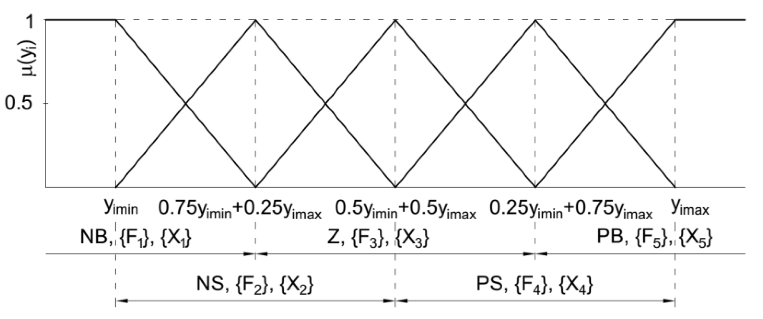
It is necessary to build a function of linear form (right trapezoid, triangle, left trapezoid) of the position error ei, the velocity error e ˙ i , and the amount of force/torque adjustment of joint i shown in Figure 4.
The membership function of yi (yi = ei, e ˙ i , ui; i = 1, …, 8) in the NB fuzzy set (Figure 4) is calculated according to (36).
μ ( y i ) = { 1 ; y i y i min y i 0.75 y i min 0.25 y imax 0.25 y i min 0.25 y imax ; y i min < y i 0.75 y i min + 0.25 y i max
The membership function of yi (yi = ei, e ˙ i , ui; i = 1, …, 8) in the NS fuzzy set (Figure 4) is calculated according to (37).
μ ( e i ) = { y i y i min 0.25 y i min + 0.25 y imax ; y i min y i 0.75 y i min +   0.25 y i max y i 0.5 y i min 0.5 y imax 0.25 y i min 0.25 y imax ; 0.75   y imin +   0.25 y i max y i 0.5 y imin +   0.5 y i max
The membership function of yi (yi = ei, e ˙ i , ui; i = 1, …, 8) in the Z fuzzy set (Figure 4) is calculated according to (38).
μ ( y i ) = { y i 0.75 y i min 0.25 y imax 0.25 y i min + 0.25 y imax ; 0.75 y i min + 0.25 y i max y i 0.5 y i min + 0.5 y i max y i 0.25 y i min 0.75 y imax 0.25 y i min 0.25 y imax ; 0.5 y i min + 0.5 y i max y i 0.25 y i min + 0.75 y i max
The membership function of yi (yi = ei, e ˙ i , ui; i = 1, …, 8) in the PS fuzzy set (Figure 4) is calculated according to (39).
μ ( y i ) = { y i 0.5 y i min 0.5 y imax 0.25 e i min + 0.25 e imax ; 0.5 y i min + 0.5 y i max y i 0.25 y i min + 0.75 y i max y i y imax 0.25 y i min 0.25 y imax ; 0.25 y i min + 0.75 y i max y i y i max
The membership function of yi (yi = ei, e ˙ i , ui; i = 1, …, 8) in the PB fuzzy set (Figure 4) is calculated according to (40).
μ ( y i ) = { y i 0.25   y i min 0.75 y imax 0.25 y i min + 0.25 y imax ; 0.25   y i min + 0.75 y i max y i < y i max 1 ; y i y i max
From the above, we realize that input and output vector signals are position errors e(t), velocity errors e ˙ ( t ) , and amount of torque adjustment u(t) of joints of the robot system within the real (explicit) physical value domain identifying them as different, but with the same linguistic value name.

5.3. Set up the Control Laws

Based on the input variables that are joint position errors e(t) and velocity errors e ˙ ( t ) , we develop a fuzzy rule table to calculate the adjustment amount of joint force/torque u(t). At the machining time, the input variables are signals of position errors e(t), velocity errors e ˙ ( t ) of joints within the physical domain {X1, …, X5} of a fuzzy set, represented by a linguistic value in the domain {NB, NS, Z, PS, PB} for each variable. The controller will generate a signal to control the amount of force/torque adjustment u(t) within the physical domain {X1, …, X5}, represented by a linguistic value in the domain {NB, NS, Z, PS, PB} and this u(t) signal corrects the input values of coordinate errors ei, velocity errors e ˙ i of joints approaching the physical value domain described by the linguistic value Z.
So, from the two input variables e(t), e ˙ ( t ) , along with 5 linguistic values of each variable, a rule system will be set up inclusive of 52 = 25 control rules for the combination of variables e(t), e ˙ ( t ) , as Table 3.
The formula to set the fuzzy compositional rule system for the fuzzy controller (41).
R : U i = 1 n   R i R i :   [ ( e ( t ) e ˙ ( t ) ) u ( t ) ]   , i = 1 , , 25
From Table 3 and Formula (41), there is the fuzzy compositional rule system (42) including fuzzy conditional statements:
{ If   e ( t )   is   NB   and   e ˙ ( t )   is   NB   then   u ( t )   is   PB   or If   e ( t )   is   NB   and   e ˙ ( t )   is   NS   then   u ( t )   is   PB   or If   e ( t )   is   PB   and   e ˙ ( t )   is   PB   then   u ( t )   is   NB  

5.4. Set up the Compositional Rule of Inference for the Fuzzy Controller

At each machining time, the input control signals of position errors e(t), velocity errors e ˙ ( t ) are always within two physical value domains, set up by two fuzzy sets, represented by two linguistic values of the domain {NB, NS, Z, PS, PB}. Therefore, it is necessary to determine the Compositional Rule of Inference. We find in turn the membership function value of output signals which is the amount of force/torque adjustment u(t) of each Compositional Rule Rk (k = 1, …, 25) and the rule system for the input control signals of coordinate errors e(t), velocity errors e ˙ ( t ) of the controller. Select the method to execute the Compositional Rule of Inference according to Mamdani composition MAX-MIN Rule (43) and (44).
F u = U i = 1 25 F u i   ;   μ F u ( y ) = V i = 1 25 μ F u i ; F i   =   ( F e , F de ) R i   ;   ( de = e ˙ )
μ F u i ( y ) = α i μ F u i ( y )   ;   α i = min { max y ( μ F e ( y ) μ F e i ( y ) ) , max y ( μ F de ( y ) μ F d e i ( y ) ) }
Use Rule (43) and (44), in turn, to determine the membership function value for each Compositional Rule and total Compositional Rule system. The output result of each Compositional Rule is the membership function value corresponding to the fuzzy set F’ (note that each membership function value corresponds to a fuzzy set F′i and the membership function value of the whole system corresponds to the general fuzzy set F’), the fuzzy set F’ is in 5 fuzzy sets represented by 5 linguistic values of the domain {NB, NS, Z, PS, PB}.

5.5. Defuzzification

The defuzzification is to determine the explicit (crisp) value y’ of the output (the amount of force/torque adjustment u(t) of joint) from the membership function value of the fuzzy set F’. Use the center of area method (COA) for defuzzification to the fuzzy controller of the robot system when surface shaping machining. This method is easy to apply, involving all output fuzzy sets of the Compositional Rule of Inference. The results of this method are highly accurate (45).
y = S y μ F ( y ) d y S μ F ( y ) d y
where y’ is the actual output value taken in accordance with the abscissa of the domain central point enclosed by membership function constituting (line) with the horizontal axis and S’ is the domain defining the fuzzy set F’. Figure 5 shows the principal structure of the fuzzy controller.
Applying the fuzzy logic as presented, this paper proposes to set up a fuzzy controller for a robot in a milling process based on the incomplete dynamic model, which means ignorance of the cutting force determination. The control block of the robot controller has a double structure consisting of an outer loop that is a fuzzy control block to determine the adjustment value based on the erroneous information of joint positions and velocities; and the inner loop is the inverse dynamics calculation block from the robot dynamic model, in which there is no cutting force component. Figure 6 shows a SIMULINK model representing the fuzzy controller for the robot system. Figure 7 shows a double-loop structure of the control block in the fuzzy controller, enabling the calculation of driving force.

6. Simulation Results

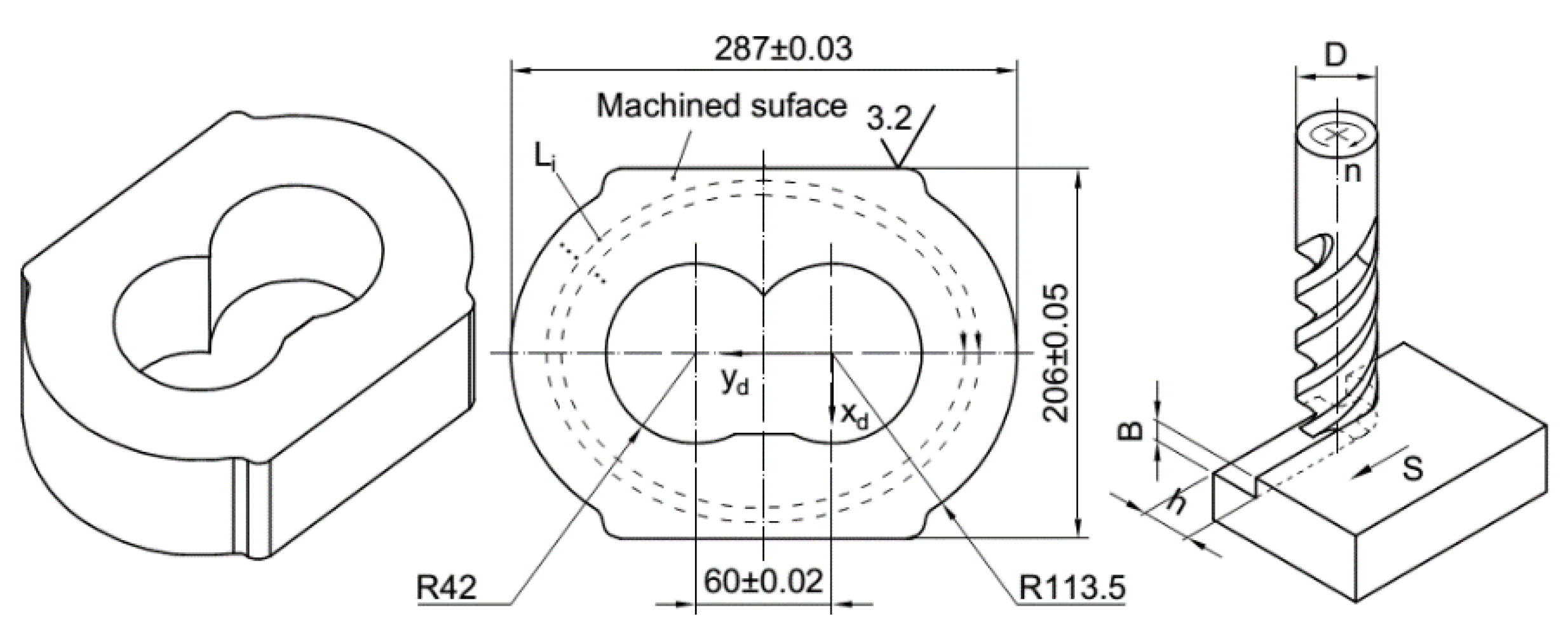
In order to verify the quality of the designed controller, this section presents the application of a robot carrying out the down milling process of a mold prototype of a hydraulic pump’s central housing, which is made of Ti6Al4V titanium alloy material. The machining trajectory is the path Li, which represents the milling path of the cutter head moving from outside to inside to complete the machining surface (Figure 8). The cutter is an end mill cutter that has four cutting edges/flutes, with a 20 mm diameter (Figure 9).
The parameters of geometric, kinematic and dynamic of the robot, platform and workpiece are determined and created as the input parameter file.
The cutter parameters and the milling process parameters are shown in Table 4, where Z is the number of cutting edges (flutes) of the cutter, vc is cutting speed, vr is the relative velocity between the tool and the workpiece, Sz is the feed rate on a cutting edge, B is milling width (B = 2.2 mm) and h is milling depth (h = 15 mm).
Assume that with the two methods of calculation and selections, the cutting force coefficients in (25) are shown in Table 5 and the results of cutting force calculation according to the empirical formula are shown in Figure 10. In particular, Figure 10 (a)÷(d), respectively, represent cutting forces in the x, y, z directions and the torque in z direction of the tool frame. The small torque components in x and y directions should be ignored.

6.1. Simulation of Inverse Dynamics + PD Controller

The Inverse Dynamics + PD controller is designed as shown in Section 4. Here, the coefficient matrices of proportional gain KP and derivative KV are selected in accordance with (46) and (47).
K P = diag { 22500 , 22500 , 22500 , 22500 , 16900 , 16900 , 16900 , 16900 }  
K V = diag { 300 , 300 , 300 , 300 , 260 , 260 , 260 , 260 }
In order to illustrate this, suppose that in the output block (robot block) of the Inverse Dynamics + PD controller in Figure 3, the cutting forces are precisely determined in accordance with the cutting force coefficients in case 1 of Table 5. The simulations are carried out for two cases where the cutting force in the input control block is calculated according to the corresponding coefficients in the two cases of Table 5, respectively. For more convenience, the simulation results that correspond to the above two cases are called PD1 and PD2.
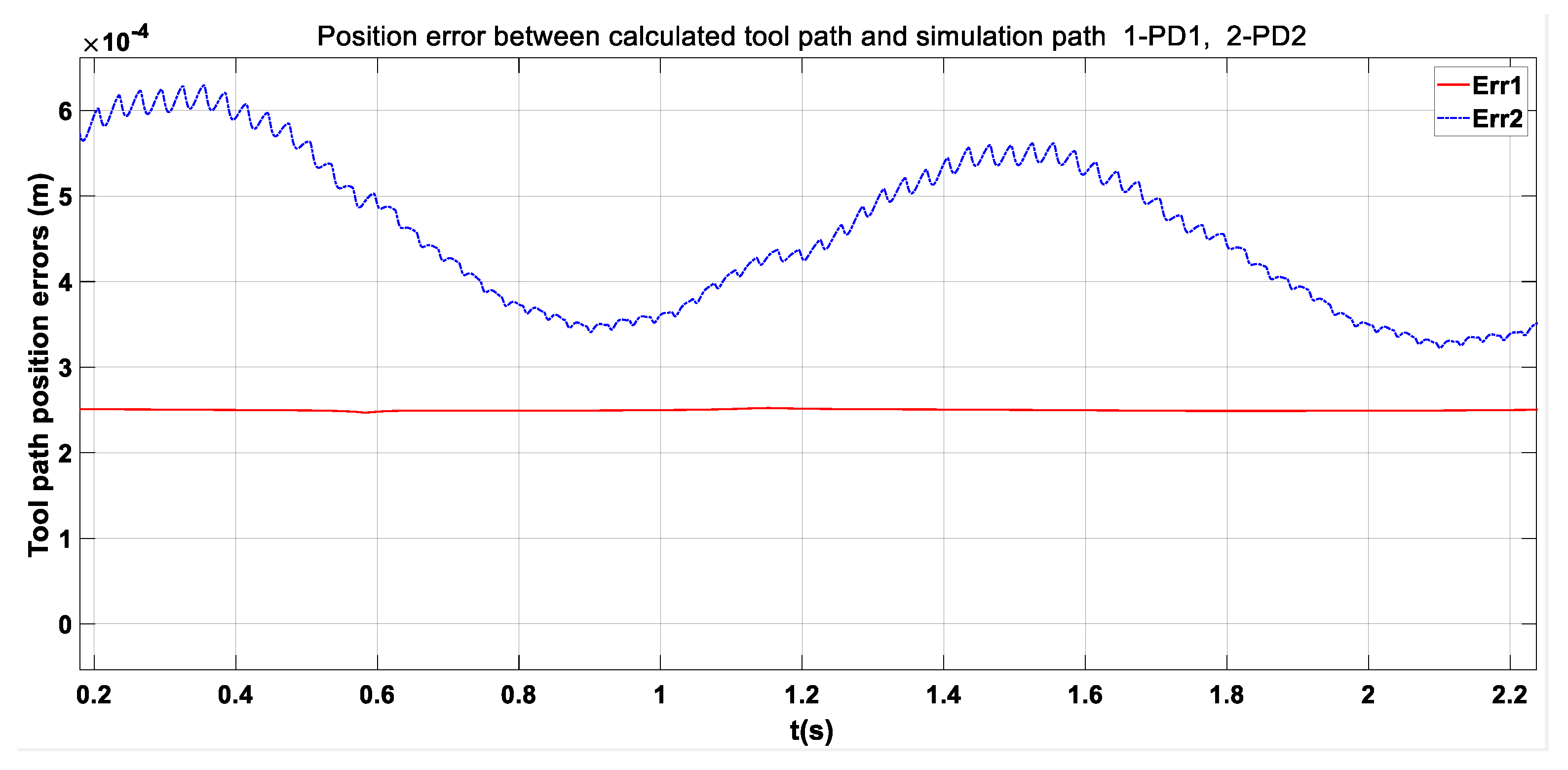
The simulation results are shown in Figure 11. In particular, Figure 11a represents the position error of first joint in comparison with the desired trajectory. Similarly, Figure 11b–h represent the position errors of the second, third,..., eighth joints respectively. The graphs that represent the errors of joint positions show the different errors corresponding to each joint. The errors of the joints that are near the end effector are greater than that of the far ones. Summarizing the joint position errors, we get the errors of the operational point of the cutting point of the tool with respect to the toolpath. Figure 12 shows the error of trajectory of the cutting point of the tool in comparison with the set trajectory as the toolpath. We realize that the trajectory error of PD1 is smaller than that of PD2 because PD1 is corresponding to the assumption of calculating cutting forces precisely.
Thus, with the analysis and the choice of different cutting force coefficients, the control results will be different and affect the machining precision of the robot significantly.

6.2. Simulation of the Fuzzy Controller

Depending on the given data of the kinematic, dynamic, etc., parameters, the physical value domain of input and output terms of the fuzzy controller are estimated as shown in Table 6.
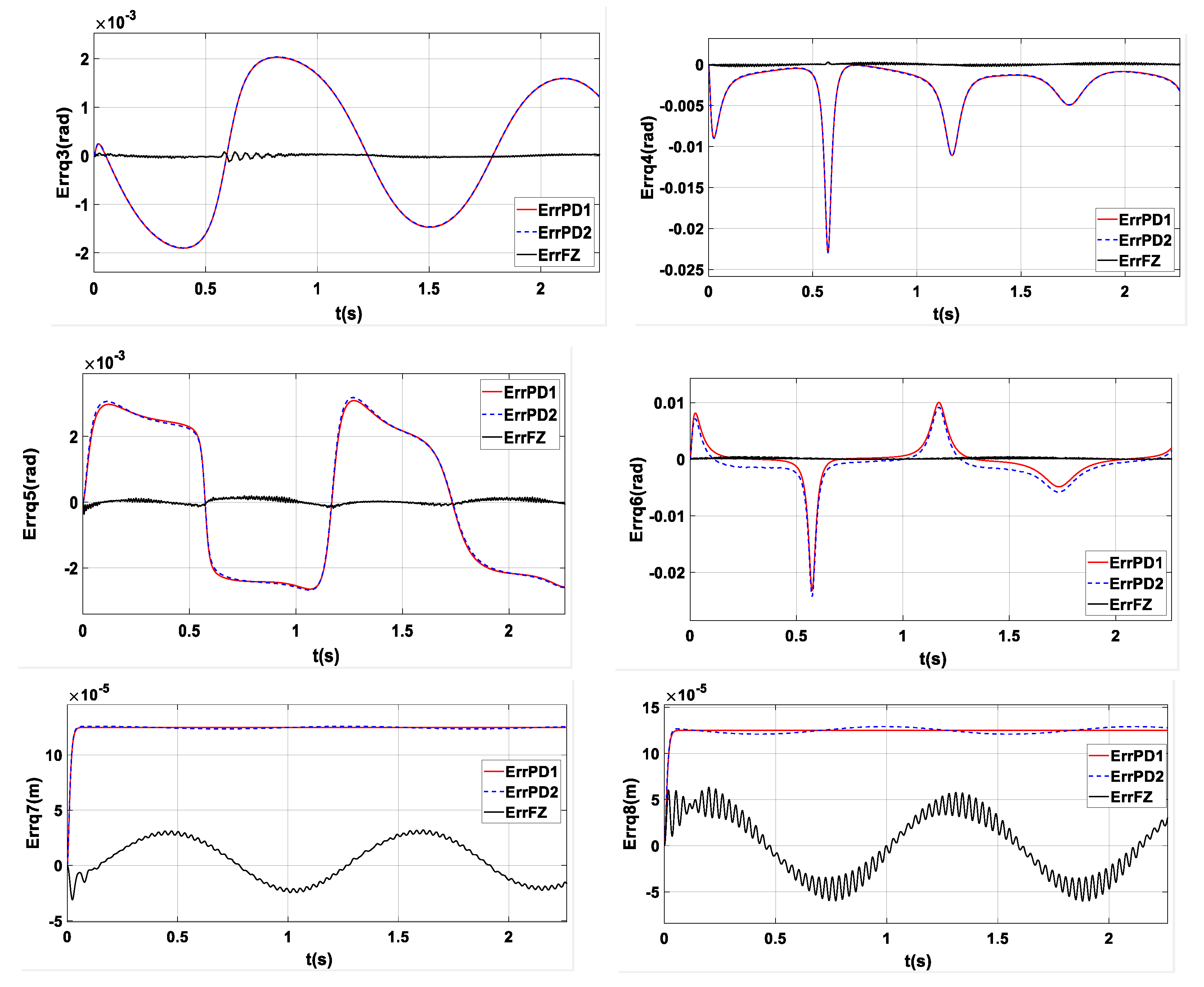
Figure 13 is the graph representing the comparison of joint position errors of the robot between the fuzzy controller and the two cases of the Inverse Dynamics + PD controller.
Figure 14 shows the trajectory error of the cutting point of the tool in the operational frame Odxdydzd, with the lines representing the error of the fuzzy controller, and the two cases of Inverse Dynamics + PD controller.
One can see that the joint position errors of the fuzzy controller are smaller than that of the PD1 and PD2 controllers.
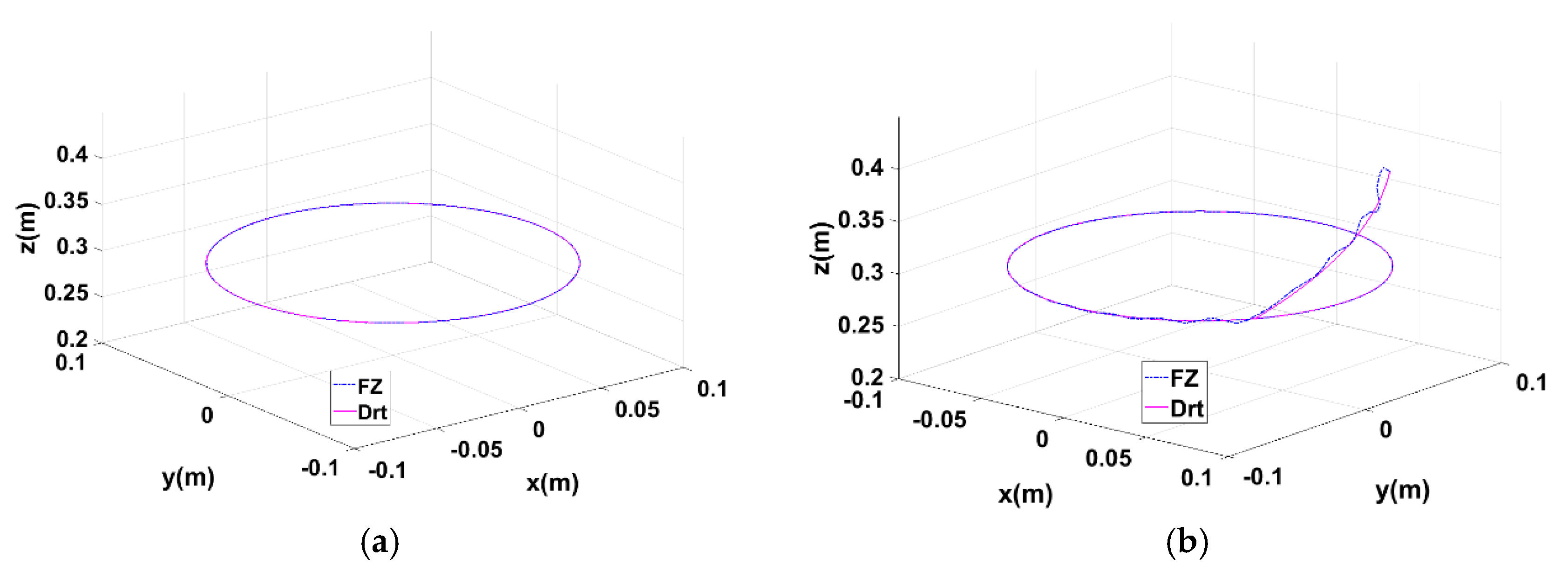
Figure 15a shows the trajectory of the cutting point of the tool in the operational frame. Due to small errors, the desired and actual trajectories of the fuzzy controller and Inverse Dynamics + PD controller are approximately coinciding.
To verify the adjustment capability of the fuzzy controller, the simulation of the fuzzy controller is performed by the initial value of the trajectory as a deviation of the desired values.
Figure 15b shows the asymptotical and convergent process of the trajectory of the cutting point from the initial deviation to coincide with the toolpath (desired trajectory) in the milling process.
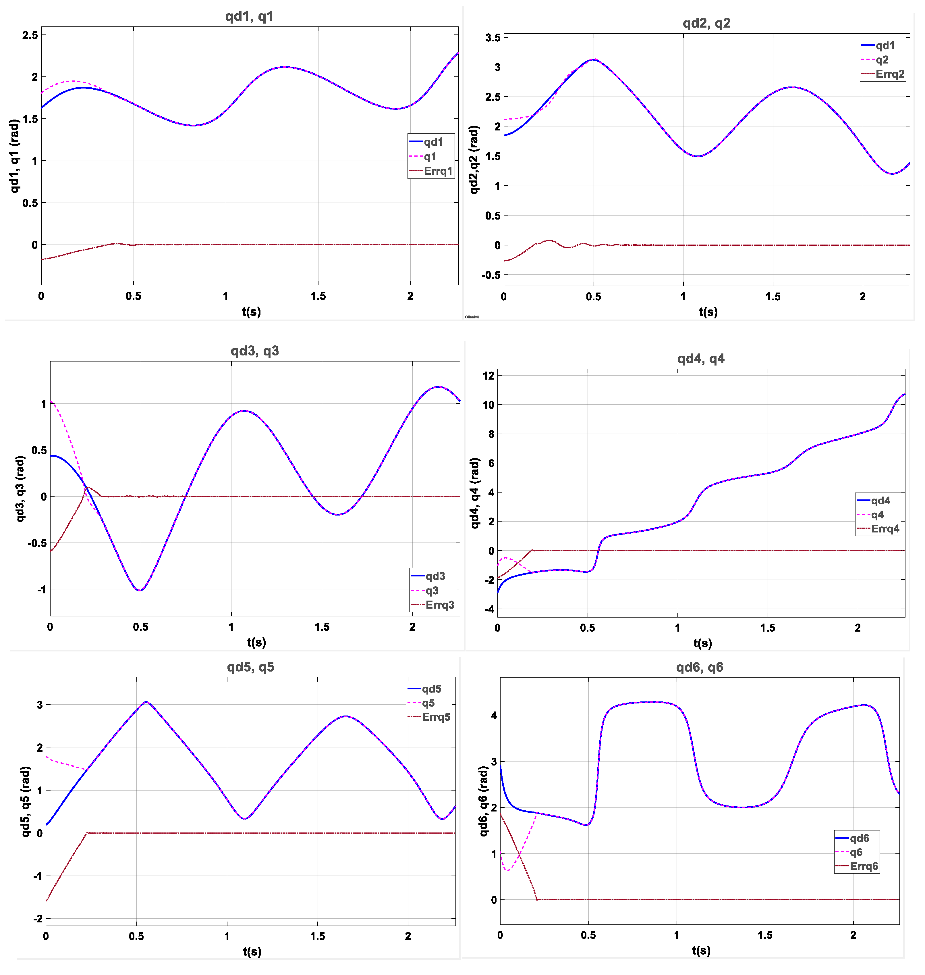
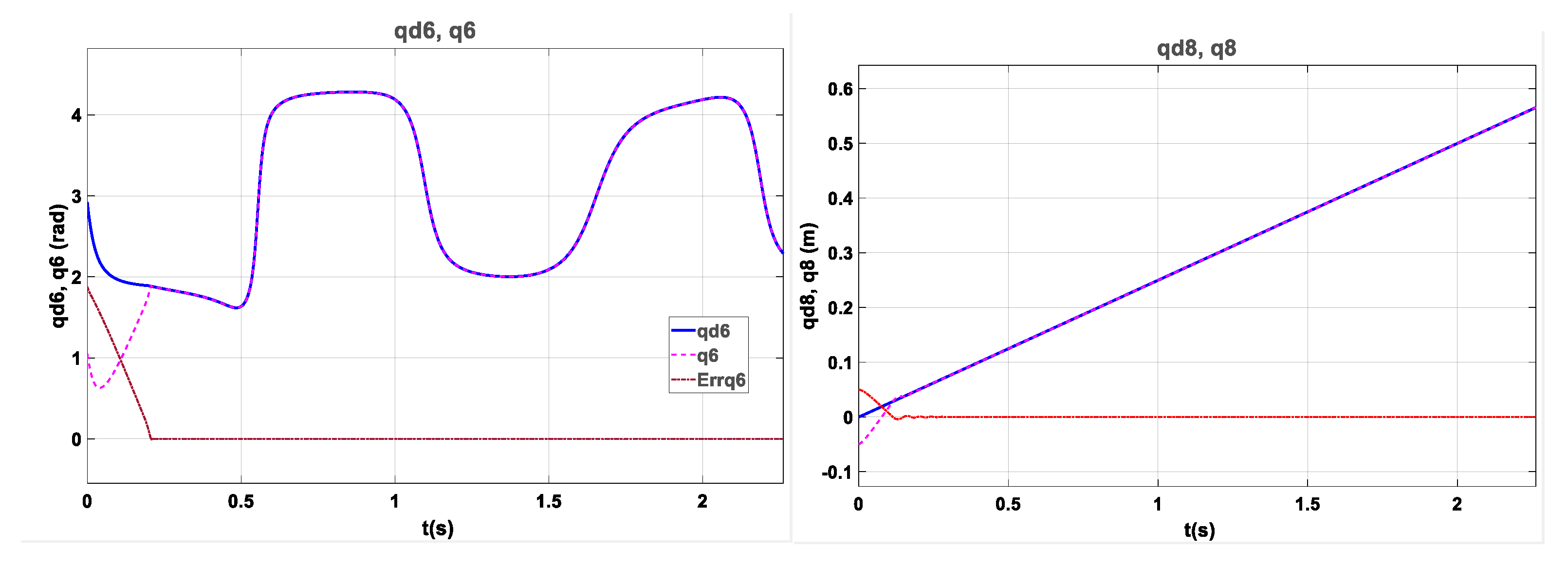
Figure 16 shows the simulation result of the fuzzy controller with initial trajectory error, time history of the joint positions, with the splines that represent the desired, actual trajectories and errors.
From the results, it can be seen that the fuzzy controller is able to control the system to the required state when there are perturbations.
In general, the simulated results show that with the assumption of ideal computed cutting forces, the Inverse Dynamics + PD explicit controller and fuzzy controller give accurate control results.

6.3. Stability Analysis

As mentioned, the designed fuzzy controller is a Mamdani type fuzzy controller, in which the development of fuzzy rule is based on the rules of the PD controller. In general, such a controller has good stability except perturbations.
The input signals of the controller include the joint position errors e(t) and the joint velocity errors e ˙ ( t ) , and the output signal of the controller is the adjustment amounts of the joint driving forces/torques u(t) at each machining instant. A good fuzzy control rule system including the above-mentioned rules will ensure that the calculation of the output value is consistent with the change of input signal and there is less possibility of overshoot. The numerical simulation results show this fact.
On the other hand, the input signal that can greatly change the output quantity is the physical value domain of driving force. Numerical experiments show that when the physical value domain of the driving force is selected at a smaller level than the value to be reached, the control simulation results are not good, with large errors, which are understandable. When the domain of physical values is expanded, the errors decrease, and when the physical value domain is large enough to cover all the necessary values of the driving force, the control accuracy will be good, as shown by the simulation results. The next question will be whether increasing the input signal by expanding the domain of physical values without control, i.e., when the value domain is selected as too large, the value of the output driving force may greatly increase? The fuzzy Inference and Defuzzification show that the output physical value of a variable depends on the input physical value domain and the membership function value of such variable. As the physical value domain increases, the output value increases but non-linearly. Numerical experiments in the direction of gradually expanding the domain of input physical values so that the physical value of the output u(t) increases gradually to the appropriate value, we realize: The error of e(t), e ˙ ( t ) reduction; the membership value of linguistic variables corresponding to the large value of the output u(t) decreases; membership values of linguistic variables with small values increase. In the fuzzy set [NB, NS, Z, PS, PB], the membership value of u(t) corresponding to Z is fast progressing to 1, other values decrease and even the NB, PB values almost go to 0 in the first steps. Based on this and based on the fuzzy inference formula, it is easy to see that the growth rate of the physical value of the output u(t) decreases and the slope of the graph decreases. The slope of the graph gradually reaches 0, the graph is horizontal, then u(t) does not increase. Above that limit, if the physical value domain of the input u(t) continues to rise too high, the physical output value u(t) does not continue to increase, but the controller error will increase again.
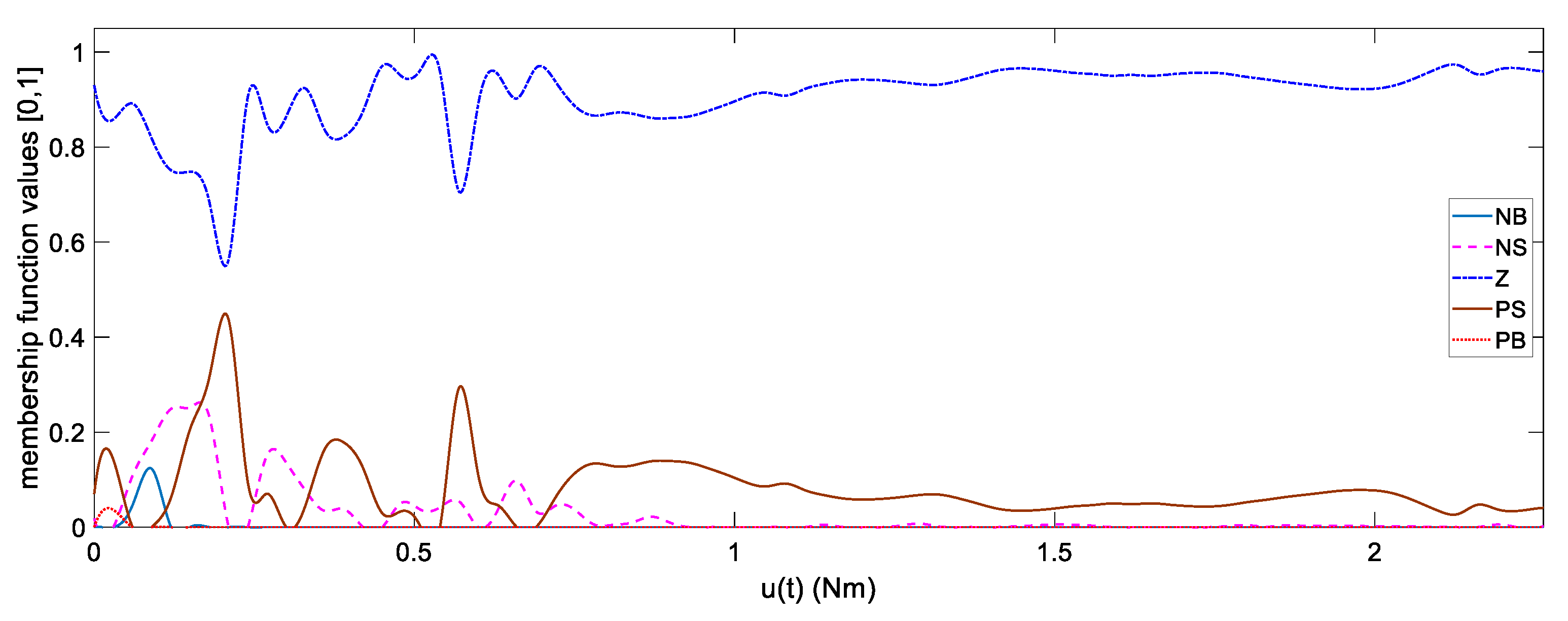
Figure 17 shows the membership function values corresponding to [NB, NS, Z, PS, PB] of the fuzzy set u(t), with the physical value domain of u(t) selected as in Table 6. The membership function value corresponding to NB, PB is almost zero, with Z close to 1. The membership function values corresponding to NS and PS of the physical value u(t) are opposite the sign and adjust the physical output value u(t).
An increase of the physical value domain of u(t) by 3 times obtains the results shown in Figure 18. Membership function values corresponding to NS, PS are about 3 times smaller than the values shown in Figure 17.
Therefore, thanks to the integration of expert knowledge, the fuzzy rules are chosen, then there will be a reasonable upper bound value for the physical value domain of control output signal. At that time, it is possible to arbitrarily select the input physical value domain to get good control results without fear of instability because there is no excessive increase of driving force. Numerical experiments are carried out when control accuracy is almost the best. In this case, when expanding the physical value domain of the driving force by 5 times, the result shows that there are some early points of the control process, when the system is in the start-up phase, that the driving force increases by about (35%÷45%). However, with the entire control process on the operating trajectory, the driving force has no significant change and control accuracy is guaranteed. Thus, with the experiment mentioned above, it is feasible to select a value domain smaller than the upper bound limit.
In addition, through the mentioned numerical simulation results, the controller can return the system to trajectory when there are errors by disturbance.
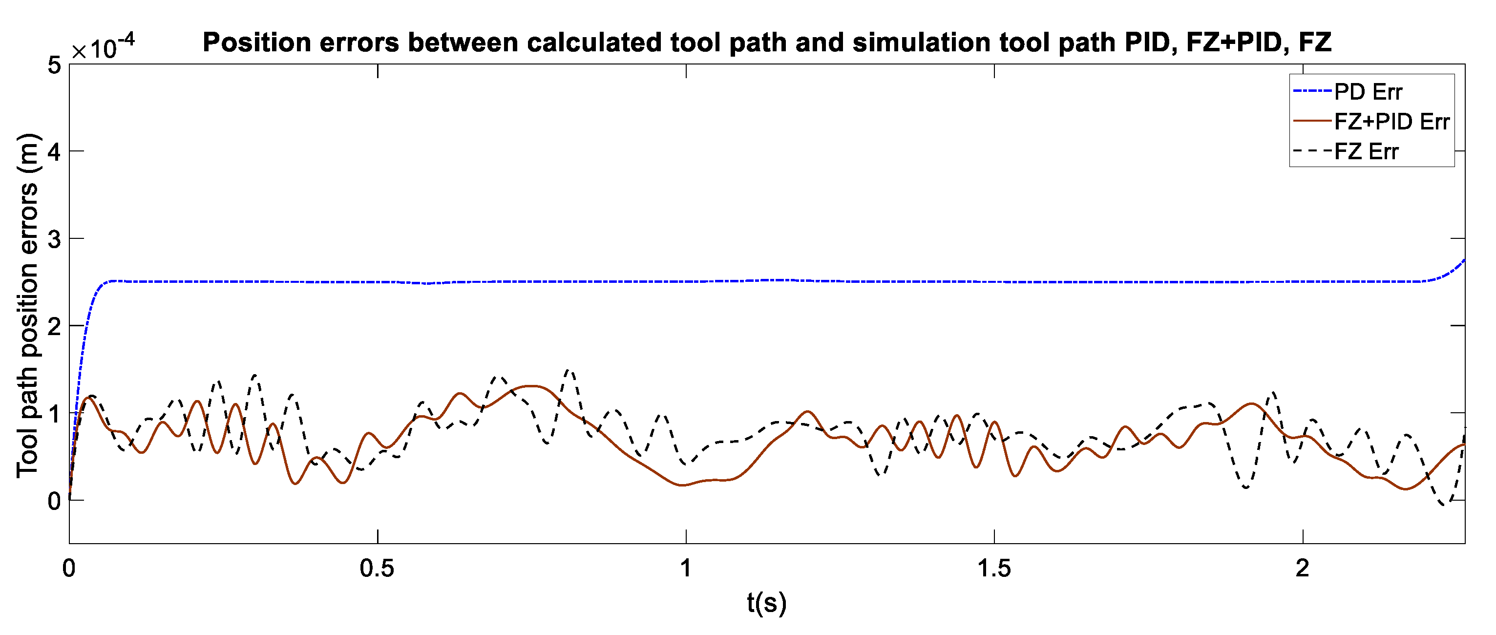
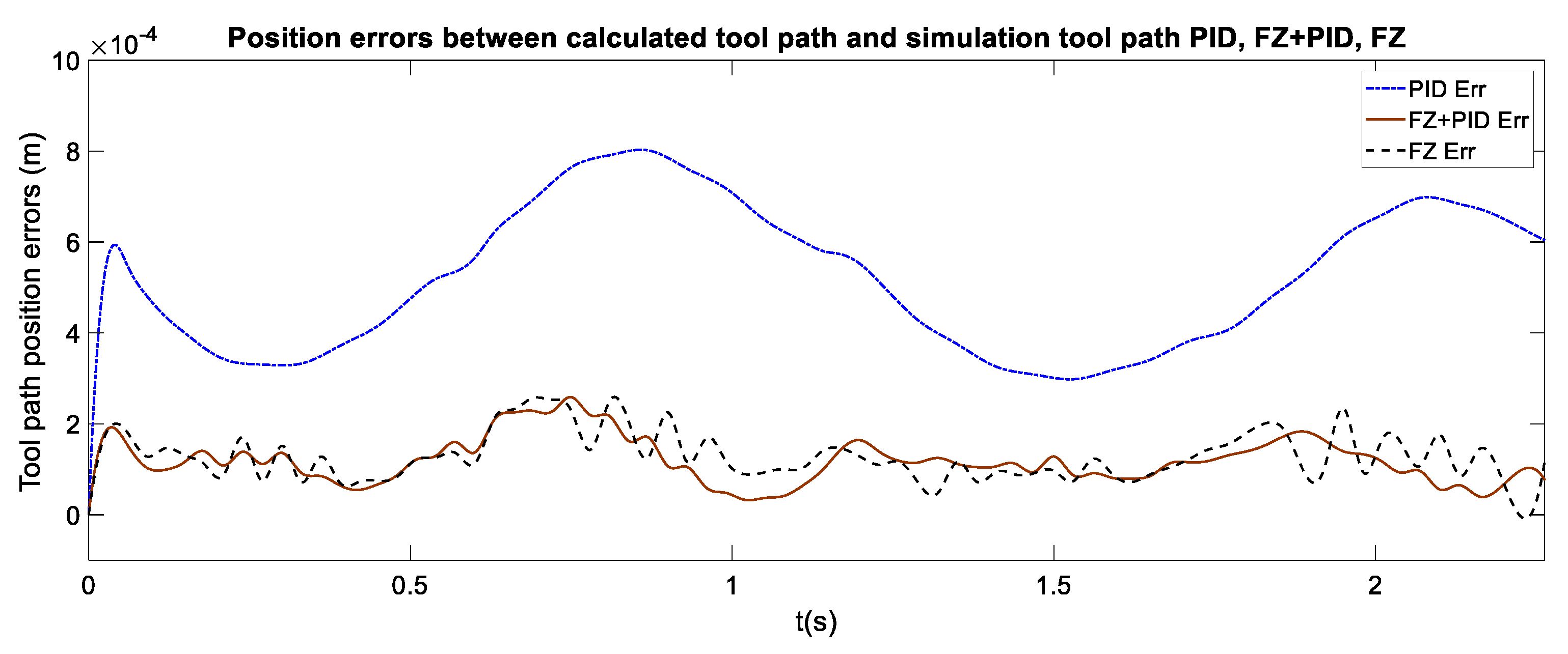
Compare the fuzzy controller (FZ) with a fuzzy controller integrated with PID (FZ + PID) shown in Figure 19 and Figure 20.
The result shows that the accuracies of Fuzzy and Fuzzy + PID controllers are almost the same. On the other hand, with noise increasing the external load (cutting force) within 50%, the accuracy is still guaranteed and the errors are negligible. Figure 19 and Figure 20 also show the simulation results of the Inverse Dynamics + PD controller (no perturbation, Figure 19), and Inverse Dynamics + PID (with perturbation, Figure 20). The adjustment capability of the Inverse Dynamics + PID controller is found to be slower.
Thus, among many methods of ensuring the stability and accuracy of the fuzzy controller, it is possible to say:
-
the fuzzy controller has an integrated PID control unit,
-
the fuzzy controller without integrated PID unit can still be stable and ensure the accuracy, by choosing a good fuzzy rule and physical value domain of appropriate input and output variables.

7. Conclusions

The results show that the controller based on fuzzy logic can meet the requirements of accuracy and reliability. Furthermore, by neglecting the calculations of the cutting forces, it is more convenient to deal with only linear algebraic calculations in fuzzy control rules, which in turn help to greatly reduce the time and computation load and increase the efficiency of the robot control system.
From the simulation results, the fuzzy controller may be even more accurate than the explicit controller, although this is only relative because the presented controllers have not been optimized. The parameters of the above controllers have been selected “quite randomly” in simulation cases.
Theoretically, the explicit controller is accurate when the dynamic model is accurate and contains no perturbations. However, in practice, it is difficult to determine precisely all the system parameters. This leads to errors in the calculation of the control signals.
Meanwhile, the fuzzy controller computes the control law based on the input and output signal errors and the fuzzy rule. Thus, the calculation results can be flexibly adjusted based on the input and output signal errors. This explains the possibility that the fuzzy controller may be more accurate than the explicit controller. In addition, the last simulation result with initial deviation of the trajectory shows that the fuzzy controller is able to control the system to the required state when there are perturbations.
The method of developing fuzzy rules and determining the physical value domain implemented in the article gives good simulation results of the fuzzy controller, which can be applied for designing the fuzzy controller for milling robots.
Difficulties in cutting force calculation and accurately determining the dynamic quantities for complex structural robot systems are always a challenge. Besides, one cannot compensate for all the perturbations such as noise and vibrations occurring due to interactions when the robot is machining or from the environment. Therefore, it is not possible to design an ideal explicit controller. Finding methods to eliminate the aforementioned factors when applying robots in machining is indispensable and compulsory. The controller based on fuzzy logic has been validated to be feasible and reliable via simulation results. It can be developed in practise to overcome the aforementioned uncertainty.

Author Contributions

Methodology, conceptualization and formal analysis, K.B.P.; investigation, K.B.P., H.T.H. and S.V.H.; survey the backgrounds, K.B.P., H.T.H. and S.V.H.; design and collect the preprocessing data, K.B.P., H.T.H.; visualization, writing–original draft, K.B.P., H.T.H.; writing–review & editing, K.B.P.; software, K.B.P.; check the draft, H.T.H. and S.V.H.; discussion and estimation the eficiency of this methodology, K.B.P., H.T.H. and S.V.H.; layout editing, H.T.H. All authors have read and agreed to the published version of the manuscript.

Funding

This research received no external funding.

Conflicts of Interest

The authors declare no conflict of interest.

Appendix A. Summary Fuzzy Logic

Unlike the crisp control that works based on a crisp logic, i.e., binary logic, the fuzzy controller works based on fuzzy logic, implementing many-valued or infinite-valued logic. The basis of crisp logic is that the crisp set has rigid boundaries while the fuzzy logic depends on fuzzy set with soft boundaries. The fuzzy set enables us to represent the real world easily and closely to human thinking. Crisp logic and fuzzy logic are mathematical languages, crisp sets and fuzzy sets include objects, elements, etc., and they are the basis for the mathematical operations. In the theories of fuzzy set, fuzzy logic develops a pretty large mathematical basis for performing mathematical operations on fuzzy sets. Accordingly, firstly, the fuzzy set elements are assigned a linguistic variable in which the linguistic values represented by the element’s membership function on the fuzzy set. Based on the universe of discourse, by quantitative or qualitative inferences, the linguistic value of a linguistic variable is determined. In fuzzy control, this process is called fuzzification process. In order for fuzzy inference to be performed with linguistic variables on fuzzy sets, the tools are developed. Firstly, characteristic parameters of fuzzy set; membership function to determine membership grade of a variable of an element in a fuzzy set. The Inferences: fuzzy relations; fuzzy rule base; Compositional Rule of Inferences… In fuzzy control, these tools are used to perform two main functions: implication and composition of fuzzy rules to come to desired results. This process plays an important role in the fuzzy controller (Appendix B and Figure A1). The physical system only receives and performs commands by physical values, therefore, defuzzification is the process of converting linguistic values into physical (crisp) values based on fuzzy inferences. Accordingly, the fuzzy controller operates in a process with three above-mentioned modules (Appendix B).
Fuzzy logic is a language, a mathematical language, like any other language we know. The elements on which fuzzy logic depend is called fuzzy set and it is also alternatively called the fuzzy algebra. Fuzzy logic is essentially a mixture of various mathematical languages to define another new language as fuzzy logic. Let X be a non-empty set (called the universal set or the universe of discourse or simply domain), which is a set that has all possible members of a particular domain.
A Fuzzy Set F is determined in universal set X in which each element is an ordered pair (x, μF(x)), where: μF: X → [0, 1]. Logical mapping μF is considered as membership function of fuzzy set F.
Characteristic parameters of fuzzy set:
The support (defined domain) of fuzzy set F (defined on the set X) is the crisp subset and defined as
Supp ( F ) = { x X : μ F ( x ) > 0 }
The core (trusted domain) of a fuzzy set F (defined on the set X) is the crisp subset and defined as
Core ( F ) = { x X : μ F ( x ) = 1 }
The height (h) of fuzzy set F (defined on the set X) is the maximum membership function value attained by any point:
h ( F ) = sup x X μ F ( F )
An α-cut of a fuzzy set F (defined on the set X) is a crisp set which its each membership function value in F are greater than or equal to α.
F α = { x X : μ F ( x ) α }
A strong α-cut of a fuzzy set F (defined on the set X) is a crisp set which its each membership function value in F are strictly greater than α.
F α + = { x X : μ F ( x ) > α }
It is easy to see that:
Core ( F ) = F 1 ; Supp ( F ) = F 0 +
The crossover point of a fuzzy set F (defined on the set X) is a point x in X such that
Crossover ( F ) = { x X : μ F ( x ) = 0.5 }
Typical Membership Function: There are many methods of establishing membership functions to determine the membership grade of an x element on a fuzzy set F, such as: triangular membership function, trapezoidal form, Gaussian form, Sign form, Sigmoidial form, Campanulate form. In fuzzy logic control, the triangular and trapezoidal membership functions are often used.
Operations on fuzzy sets: There are many operations on fuzzy sets, but in this paper we introduce three basic operations: unions, intersection of two fuzzy sets and fuzzy complementation. Consider two fuzzy sets A, B on the universe of discourse X. For a given element x of the X, these operations are introduced. Based on the definition of fuzzy union and intersection, there are many formulas that can be applied to calculate the membership function of the union or intersection of two fuzzy sets, such as the formula based on maximum rule, Lukasiewicz rule, direct sum formula, etc. Here, the formulas based on maximum and minimum rules are introduced:
Unions (max rule):
μ A B ( x ) = max { μ A ( x ) , μ B ( x ) } = μ A ( x ) μ B ( x ) ; x X
Intersection (min rule):
μ A B ( x ) = min { μ A ( x ) , μ B ( x ) } = μ A ( x ) μ B ( x ) ; x X
Complement:
μ A ¯ ( x ) = 1 μ A ( x ) ; x X
Linguistic variable: A linguistic variable is a variable that represents a physical quantity by words or sentences in natural or artificial language. A linguistic value is a natural language term which is derived using quantitative or qualitative reasoning. A fuzzy linguistic variable x will take values that are linguistic values. Thus, a variable can both be represented by physical values and linguistic values. For example, velocity variables can be represented by two value domains. The physical value domain:
V = { x R : x 0 }
The linguistic value domain:
V L = { very slow ( VL ) ,   slow ( L ) ,   normal ( M ) ,   fast ( F ) ,   veryfast ( VF ) }
Here, the universal set is the velocity set V, the fuzzy set LV is defined on set V. With a physical value x ∈ V, the membership function can be determined, corresponding to subsets of LV, and represented by vector μ as follow:
x μ = [ μ VL ( x ) ,   μ L ( x ) ,   μ M ( x ) ,   μ F ( x ) ,   μ VF ( x ) ] T
The above mapping is called the fuzzification process, in which the physical value of a variable is transformed into linguistic value.
Fuzzy relations: A fuzzy relation R on Cartesian product of universal sets U1 × U2 × … × Un is any fuzzy subset of U1 × U2 × … × Un. Thus, a fuzzy relation R is defined by a membership function
μ R ( x 1 , x 2 , , x n ) : U 1 × U 1 × U n [ 0 , 1 ]   or   μ R ( x 1 , x 2 , , x n ) [ 0 , 1 ]
If the Cartesian product is formed by just two sets U1 × U2, the relation is called a binary fuzzy relation on U1 × U2.
A relation R between fuzzy sets A and B denotes composition of A and B
R = { ( x , y ) , μ R ( x , y ) : μ R ( x , y ) = min ( μ A ( x ) , μ B ( y ) )   or   μ R ( x , y ) = μ A ( x ) μ B ( y ) }
Composition of fuzzy relations R and S: Let R, S, T be fuzzy relations on the Cartesian spaces X × Y, Y × Z, and X × Z, respectively, x ∈ X, y ∈ Y, z ∈ Z.
Union:
μ R S ( x , y ) = max { μ R ( x , y ) , μ S ( x , y ) } = μ R ( x , y ) μ S ( x , y )
Intersection:
μ R S ( x , y ) = mix { μ R ( x , y ) , μ S ( x , y ) } = μ R ( x , y ) μ S ( x , y )
Complement:
μ R ¯ ( x , y ) = 1 μ R ( x , y )
Max–Min composition:
T = R S = { ( x , y ) , max y { min ( μ R ( x , y ) , μ S ( y , z ) ) } : x x , y y , z z }
Max–Product composition:
T = R S = { ( x , y ) , max y ( μ R ( x , y ) μ S ( y , z ) ) : x x , y y , z z }
Max–Average composition:
T = R S = { ( x , y ) , max y ( μ R ( x , y ) + μ S ( y , z ) ) : x x , y y , z z }
Fuzzy rules and implications: The fuzzy implication (also known as fuzzy rule, fuzzy If-Then rule, or fuzzy conditional statement) is defined in form: “If x is A then y is B”, where A and B are two linguistic variables defined by fuzzy sets A and B on the universal sets X and Y, respectively. There are two well-known fuzzy implication rules, widely used in fuzzy system and fuzzy control:
Min operation rule (Mamdani implication rule): The fuzzy membership function of fuzzy implication
μ A B ( x , y ) = min { μ A ( x ) , μ B ( y ) } = μ A ( x ) μ B ( y )
Product operation rule (Larsen):
μ A B ( x , y ) = μ A ( x ) μ B ( y )
Fuzzy compositional rules: In this paper, the method Mamdani is introduced. The method Mamdani uses a minimum operator as a fuzzy implication operator, and max-min operator for the composition. Suppose fuzzy rule is Single-Input/Single-Output (SISO) Rule Base as R: if x is A then z is C, infer result C′ for another rule if x is A′ then z is C′, where A, C, A′ are known. When input data is a singleton such as A′ = x0,
C = A R ; μ C ( x ) = min { μ A ( x 0 ) , μ C ( z ) } = α μ C ( z ) ;   where   α = μ A ( x 0 )
When input data is fuzzy set A′,
C = A R ;   μ C ( x ) = max { min ( α , μ C ( z ) ) } = max ( α μ C ( z ) ) ; where   α = min ( μ A ( x ) , μ A ( x ) )
The α is called the “matching degree”, “satisfaction degree”, or “firing strength”.
Multi-Input/Single-Output (MISO) Rule Base:
Ri: if x is Ai and y is Bi then z is Ci, i = 1, 2, …, n. Where Ai, Bi, Ci, i = 1, 2, …, n and A′, B′ are known, the output C′ is obtained as follow:
C = i = 1 n C i   ; μ C ( z ) = V i = 1 n μ C i ; μ C i ( z ) = α i μ C i ( z )
When input data are singletons such as x = x0 and y = y0,
C i = A R i   ; α i = μ A i ( x 0 ) μ B i ( y 0 )  
When input data are fuzzy sets, A′ and B′,
C i   =   ( A , B ) R i   ; α i = min { max x ( μ A ( x ) μ A i ( x ) ) , max y ( μ B ( y ) μ B i ( y ) ) }
Defuzzification: In practical applications, the control commands work by crisp value. Therefore it is necessary to defuzzify the result of the fuzzy inference. Defuzzification is the process where the mapping is done to convert the fuzzy results into crisp values. There are many methods for defuzzification technique. This paper introduces two well-known and widely used methods in fuzzy system and fuzzy control.
Center of area method (COA):
y =   S y μ C ( y ) d y S μ C ( y ) d y ;   or   y =   J = 1 n y j μ C ( y j ) j = 1 n μ C ( y j )
where, the first formula for the case y is continuous; S is the Support (defined domain) of fuzzy set C′; n is the number of quantization levels of the output; C is a fuzzy set defined on the output dimension (y).
Mean of maximum method (MOM):
y = j = 1 k y j k
where, yj is the control action whose membership functions reach the maximum; k is the number of such control actions.

Appendix B. Fuzzy Logic Controller

In general, a fuzzy controller has three main components (Figure A1):
  • The interface consists of a fuzzification module and some additional ones for solving problems such as generating trajectories of motion, differentiation, integration… Fuzzification is the method of translating a crisp quantity into a fuzzy quantity.
  • The compositional device consists of two main modules that are fuzzy rules and the inference mechanism. Two approaches for construction of fuzzy logic control are Mamdani and Takagi—Sugeno’s approaches. This paper uses the Mamdani approach in developing fuzzy rules as well as fuzzy inference. In order to develop fuzzy rule systems, the essential nature and key characteristics of the object being controlled are analyzed based on expert knowledge and experience. The effectiveness of these based on the fuzzy approach are the most important factors, i.e., deciding whether fuzzy rules are good or not, to ensure good quality control.
  • Defuzzification is the operation process that inverses the process of fuzzification, where the fuzzy results are converted into crisp values for the controller to perform physical operations.
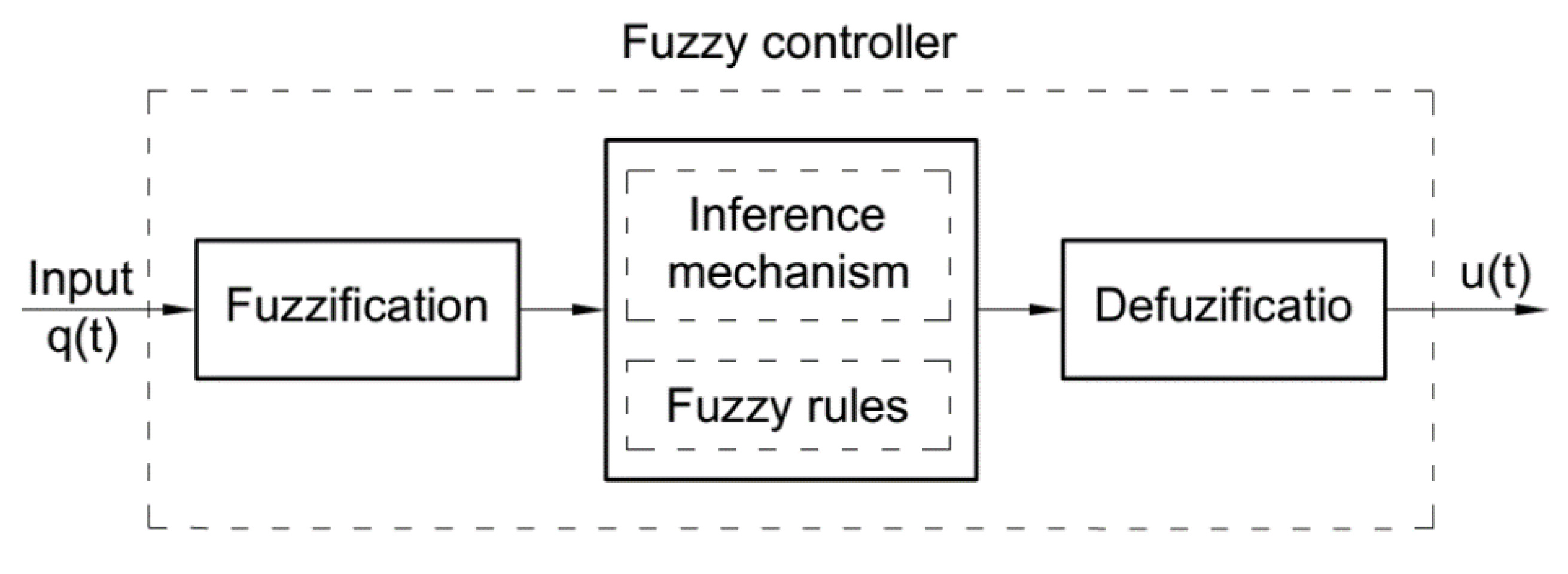
Figure A1. A general fuzzy controller.
Applsci 10 01685 g0a1

References

  1. Appleton, E.; Williams, D.J. Industrial Robot Applications; Springer Science & Business Media: Berlin, Germany, 2012. [Google Scholar]
  2. Ji, W.; Wang, L. Industrial robotic Machining: A review. Int. J. Adv. Manuf. Technol. 2019, 103, 1239–1255. [Google Scholar] [CrossRef] [Green Version]
  3. Pandremenos, J.; Doukas, C.; Stavropoulos, P.; Chryssolouris, G. Machining with robots: A critical review. In Proceedings of the DET 2011, Athens, Greece, 28–30 September 2011; pp. 1–8. [Google Scholar]
  4. Petko, M.; Gac, K.; Góra, G.; Karpiel, G.; Ochoński, J.; Kobus, K. CNC system of the 5-axis hybrid robot for milling. Mechatronics 2016, 37, 89–99. [Google Scholar] [CrossRef]
  5. Cen, L.; Melkote, S.N. CCT-based mode coupling chatter avoidance in robotic milling. J. Manuf. Process. 2017, 29, 50–61. [Google Scholar] [CrossRef]
  6. COMET, E.U. FP7-Project: Plug-and-Produce Components and Methods for Adaptive Control of Industrial Robots Enabling Cost Effective, High Precision Manufacturing in Factories of the Future. Available online: http://www.cometproject.eu (accessed on 1 September 2010).
  7. Petko, M.; Karpiel, G.; Gac, K.; Góra, G.; Kobus, K.; Ochoński, J. Trajectory tracking controller of the hybrid robot for milling. Mechatronics 2016, 37, 100–111. [Google Scholar] [CrossRef]
  8. Gołda, G.; Kampa, A. Modelling of cutting force and robot load during machining. In Advanced Materials Research. Trans Tech Publ. 2014, 1036, 715–720. [Google Scholar]
  9. Cen, L.; Melkote, S.N. Effect of robot dynamics on the machining forces in robotic milling. Procedia Manuf. 2017, 10, 486–496. [Google Scholar] [CrossRef]
  10. Perrusquía, A.; Yu, W.; Soria, A. Position/force control of robot manipulators using reinforcement learning. Ind. Robot Int. J. Robot. Res. Appl. 2019, 46, 267–280. [Google Scholar] [CrossRef]
  11. Lacerda, H.B.; Lima, V.T. Evaluation of cutting forces and prediction of chatter vibrations in milling. J. Braz. Soc. Mech. Sci. Eng. 2004, 26, 74–81. [Google Scholar] [CrossRef] [Green Version]
  12. Leonesio, M.; Villagrossi, E.; Beschi, M.; Marini, A.; Bianchi, G.; Pedrocchi, N.; Isaev, A. Vibration analysis of robotic milling tasks. Procedia Cirp 2018, 67, 262–267. [Google Scholar] [CrossRef]
  13. Wang, G.; Dong, H.; Guo, Y.; Ke, Y. Dynamic cutting force modeling and experimental study of industrial robotic boring. Int. J. Adv. Manuf. Technol. 2016, 86, 179–190. [Google Scholar] [CrossRef]
  14. Lazoglu, I. A new identification method of specific cutting coefficients for ball end milling. Procedia Cirp 2014, 14, 182–187. [Google Scholar]
  15. Ghorbani, H.; Moetakef-Imani, B. Specific cutting force and cutting condition interaction modeling for round insert face milling operation. Int. J. Adv. Manuf. Technol. 2016, 84, 1705–1715. [Google Scholar] [CrossRef]
  16. Nan, C.; Liu, D. Analytical Calculation of Cutting Forces in Ball-End Milling with Inclination Angle. J. Manuf. Mater. Process. 2018, 2, 35. [Google Scholar] [CrossRef] [Green Version]
  17. Kaymakci, M.; Kilic, Z.M.; Altintas, Y. Unified cutting force model for turning, boring, drilling and milling operations. Int. J. Mach. Tools Manuf. 2012, 54, 34–45. [Google Scholar] [CrossRef]
  18. Davoudinejad, A.; Tosello, G.; Parenti, P.; Annoni, M. 3D finite element simulation of micro end-milling by considering the effect of tool run-out. Micromachines 2017, 8, 187. [Google Scholar] [CrossRef] [Green Version]
  19. Huo, D.; Chen, W.; Teng, X.; Lin, C.; Yang, K. Modeling the influence of tool deflection on cutting force and surface generation in micro-milling. Micromachine 2017, 8, 188. [Google Scholar] [CrossRef]
  20. Luo, M.; Chong, Z.; Liu, D. Cutting forces measurement for milling process by using working tables with integrated PVDF thin-film sensors. Sensors 2018, 18, 4031. [Google Scholar] [CrossRef] [Green Version]
  21. Tuysuz, O.; Altintas, Y.; Feng, H.Y. Prediction of cutting forces in three and five-axis ball-end milling with tool indentation effect. Int. J. Mach. Tools Manuf. 2013, 66, 66–81. [Google Scholar] [CrossRef] [Green Version]
  22. Wang, M.; Gao, L.; Zheng, Y. An examination of the fundamental mechanics of cutting force coefficients. Int. J. Mach. Tools Manuf. 2014, 78, 1–7. [Google Scholar] [CrossRef]
  23. Díaz-Tena, E.; Ugalde, U.; De Lacalle, L.L.; De la Iglesia, A.; Calleja, A.; Campa, F.J. Propagation of assembly errors in multitasking machines by the homogenous matrix method. Int. J. Adv. Manuf. Technol. 2013, 68, 149–164. [Google Scholar]
  24. Aydın, M.; Köklü, U. Identification and modeling of cutting forces in ball-end milling based on two different finite element models with Arbitrary Lagrangian Eulerian technique. Int. J. Adv. Manuf. Technol. 2017, 92, 1465–1480. [Google Scholar] [CrossRef]
  25. Artetxe, E.; Urbikain, G.; Lamikiz, A.; López-de-Lacalle, L.N.; González, R.; Rodal, P. A mechanistic cutting force model for new barrel end mills. Procedia Eng. 2015, 132, 553–560. [Google Scholar] [CrossRef] [Green Version]
  26. Lamikiz, A.; De Lacalle, L.L.; Sánchez, J.A.; Salgado, M.A. Cutting force integration at the CAM stage in the high-speed milling of complex surfaces. Int. J. Comput. Integr. Manuf. 2005, 18, 586–600. [Google Scholar] [CrossRef]
  27. Gonzalo, O.; Jauregi, H.; Uriarte, L.G.; de Lacalle, L.L. Prediction of specific force coefficients from a FEM cutting model. Int. J. Adv. Manuf. Technol. 2009, 43, 348. [Google Scholar] [CrossRef]
  28. Lamikiz, A.D.; De Lacalle, L.L.; Sanchez, J.A.; Salgado, M.A. Cutting force estimation in sculptured surface milling. Int. J. Mach. Tools Manuf. 2004, 44, 1511–1526. [Google Scholar] [CrossRef]
  29. Lin, X.; Wu, G.; Zhang, Y.; Cui, T.; Zhang, B.; Sun, P. The identification of the cutting force coefficients for ball-end finish milling. Int. J. Adv. Manuf. Technol. 2019, 102, 4121–4135. [Google Scholar] [CrossRef]
  30. Moges, T.M.; Desai, K.A.; Rao, P.V.M. Modeling of cutting force, tool deflection, and surface error in micro-milling operation. Int. J. Adv. Manuf. Technol. 2018, 98, 2865–2881. [Google Scholar] [CrossRef]
  31. Peng, B.; Bergs, T.; Schraknepper, D.; Klocke, F.; Döbbeler, B. A hybrid approach using machine learning to predict the cutting forces under consideration of the tool wear. Procedia Cirp 2019, 82, 302–307. [Google Scholar] [CrossRef]
  32. Zhang, X.; Yu, T.; Wang, W. Cutting forces modeling for micro flat end milling by considering tool run-out and bottom edge cutting effect. Proc. Inst. Mech. Eng. Part B J. Eng. Manuf. 2019, 233, 470–485. [Google Scholar] [CrossRef]
  33. Zadeh, L.A. Fuzzy sets. Inf. Control 1965, 8, 338–353. [Google Scholar] [CrossRef] [Green Version]
  34. Mamdani, E.H. Twenty years of fuzzy control: Experiences gained and lessons learnt. In Proceedings of the 1993 Second IEEE International Conference on Fuzzy Systems, San Francisco, CA, USA, 28 March–1 April 1993; pp. 339–344. [Google Scholar]
  35. Kumar, V.; Nakra, B.C.; Mittal, A.P. A review on classical and fuzzy PID controllers. Int. J. Intell. Control Syst. 2011, 16, 170–181. [Google Scholar]
  36. Hampel, R.; Wagenknecht, M.; Chaker, N. (Eds.) Fuzzy Control: Theory and Practice; Springer Science & Business Media: Berlin, Germany, 2013. [Google Scholar]
  37. Boutalis, Y.; Christodoulou, M.A.; Theodoridis, D.; Kottas, T. System identification and adaptive control. Theory and Applications of the Neurofuzzy and Fuzzy Cognitive Network Models; Springer International Publishing: Cham, Switzerland, 2014; 313p. [Google Scholar]
  38. Matía, F.; Marichal, G.N.; Jiménez, E. (Eds.) Fuzzy Modeling and Control: Theory and Applications; Atlantis Press: Paris, France, 2014; 288p. [Google Scholar]
  39. Hooda, D.S.; Raich, V. Fuzzy Logic Models and Fuzzy Control: An Introduction; Alpha Science International: Oxford, UK, 2017. [Google Scholar]
  40. Sharma, K.D.; Chatterjee, A.; Rakshit, A. Intelligent Adaptive Fuzzy Control. In Intelligent Control; Springer: Singapore, 2018; pp. 3–21. [Google Scholar]
  41. De Silva, C.W. Intelligent Control: Fuzzy Logic Applications; CRC press: Boca Raton, FL, USA, 2018. [Google Scholar]
  42. Lee, K.H. First Course on Fuzzy Theory and Applications; Springer Science & Business Media: Berlin, Germany, 2004. [Google Scholar]
  43. Barros, L.C.D.; Bassanezi, R.C.; Lodwick, W.A. A First Course in Fuzzy Logic, Fuzzy Dynamical Systems, and Biomathematics: Theory and Applications; Springer-Verlag: Berlin/Heidelberg, Germany, 2017; 299p. [Google Scholar]
  44. Liu, H.; Wang, T.; Wang, D. Constant cutting force control for CNC machining using dynamic characteristic-based fuzzy controller. Shock Vib. 2015, 2015. [Google Scholar] [CrossRef]
  45. Kovač, P.; Rodić, D.; Gostimirović, M.; Savković, B.; Ješić, D. Application of adaptive neuro fuzzy systems for grinding process modeling. In Proceedings of the 6th International Conference on Information Society and Technology ICIST, Society for Information Systems and Computer Networks Pub., Belgrade, Serbia, 28 February–2 March 2016; 2016; pp. 247–250. [Google Scholar]
  46. Huang, S.J.; Shy, C.Y. Fuzzy logic for constant force control of end milling. IEEE Trans. Ind. Electron. 1999, 46, 169–176. [Google Scholar] [CrossRef]
  47. Zhao, Y.; Collins, E.G. Fuzzy PI control design for an industrial weigh belt feeder. IEEE Trans. Fuzzy Syst. 2003, 11, 311–319. [Google Scholar] [CrossRef]
  48. Huang, L.; Ge, S.S.; Lee, T.H. Fuzzy unidirectional force control of constrained robotic manipulators. Fuzzy Sets Syst. 2003, 134, 135–146. [Google Scholar]
  49. Kizir, S.; BİNGÜL, Z. Fuzzy impedance and force control of a Stewart platform. Turk. J. Electr. Eng. Comput. Sci. 2014, 22, 924–939. [Google Scholar] [CrossRef]
  50. Chen, C.H.; Wang, C.C.; Wang, Y.T.; Wang, P.T. Fuzzy logic controller design for intelligent robots. Math. Probl. Eng. 2017, 1–12. [Google Scholar] [CrossRef]
  51. Stoian, V.; Ivanescu, M. Robot Control by Fuzzy Logic. In Frontiers in Robotics, Automation and Control; IntechOpen Pub.: Rijeka, Croatia, 2008; pp. 111–132. [Google Scholar]
  52. Vashisth, H.; Woo, P.Y. Application of fuzzy logic to robotic control. In Proceedings of the 1996 IEEE IECON. 22nd International Conference on Industrial Electronics, Control, and Instrumentation, Taipei, Taiwan, 9 August 1996; Volume 3, pp. 1867–1872. [Google Scholar]
  53. Chaudhary, H.; Panwar, V.; Sukavanum, N.; Prasad, R. Fuzzy PD+ I based hybrid force/position control of an industrial robot manipulator. Ifac Proc. Vol. 2014, 47, 429–436. [Google Scholar] [CrossRef]
  54. de Silva, C.W. Applications of fuzzy logic in the control of robotic manipulators. Fuzzy Sets Syst. 1995, 70, 223–234. [Google Scholar] [CrossRef]
  55. Mendes, N.; Neto, P.; Pires, J.N.; Loureiro, A. An optimal fuzzy-PI force/motion controller to increase industrial robot autonomy. Int. J. Adv. Manuf. Technol. 2013, 68, 435–441. [Google Scholar]
  56. Mendes, N.; Neto, P. Indirect adaptive fuzzy control for industrial robots: A solution for contact applications. Expert Syst. Appl. 2015, 42, 8929–8935. [Google Scholar] [CrossRef]
  57. Khoi, P.B.; Van Toan, N. Hedge-Algebras-Based Controller for Mechanisms of Relative Manipulation. Int. J. Precis. Eng. Manuf. 2018, 19, 377–385. [Google Scholar] [CrossRef]
  58. Toan, N.V.; Khoi, P.B. Fuzzy-based-admittance controller for safe natural human–robot interaction. Adv. Robot. 2019, 1–9. [Google Scholar] [CrossRef]
  59. Wakileh, B.A.M.; Gill, K.F. Use of fuzzy logic in robotics. Comput. Ind. 1988, 10, 35–46. [Google Scholar] [CrossRef]
  60. Khoi, P.B.; Van Toan, N. Optimizing Neuro-Fuzzy System for Robot Control. J. Sci. Technol. 2014, 52, 685–699. [Google Scholar]
  61. Lin, C.H.; Wang, S.H.; Lin, C.J. Interval Type-2 Neural Fuzzy Controller-Based Navigation of Cooperative Load-Carrying Mobile Robots in Unknown Environments. Sensors 2018, 18, 4181. [Google Scholar] [CrossRef] [Green Version]
  62. Van Toan, N.; Khoi, P.B. A control solution for closed-form mechanisms of relative manipulation based on fuzzy approach. Int. J. Adv. Robot. Syst. 2019, 16, 1–11. [Google Scholar] [CrossRef]
  63. Hsu, F.Y.; Fu, L.C. A new adaptive fuzzy hybrid force/position control for intelligent robot deburring. In Proceedings of the 1999 IEEE International Conference on Robotics and Automation, Detroit, MI, USA, 10–15 May 1999; Volume 3, pp. 2476–2481. [Google Scholar]
  64. Hendzel, Z.; Burghardt, A.; Gierlak, P.; Szuster, M. Conventional and fuzzy force control in robotised machining. Solid State Phenom. Trans Tech Publ. 2014, 210, 178–185. [Google Scholar] [CrossRef] [Green Version]
  65. Cuka, B.; Kim, D.W. Fuzzy logic based tool condition monitoring for end-milling. Robot. Comput.-Integr. Manuf. 2017, 47, 22–36. [Google Scholar] [CrossRef]
  66. Hsu, F.Y.; Fu, L.C. Intelligent robot deburring using adaptive fuzzy hybrid position/force control. IEEE Trans. Robot. Autom. 2000, 16, 325–335. [Google Scholar] [CrossRef]
  67. Khoi, P.B.; Van Toan, N. Application of fuzzy logic for controlling mechanisms of relative manipulation robot (MRM robot). J. Sci. Technol. 2016, 54, 385–401. [Google Scholar] [CrossRef] [Green Version]
  68. Khoi, P.B. Calculation and simulation the program motion of mechanisms of relative manipulation (MRM). J. Sci. Technol. 2009, 3, 19–28. [Google Scholar]
  69. Khoi, P.B. Kinematic problems of programming control of mechanism of relative manipulation. In Proceedings of the National Conference on Mechanics, Hanoi, Vietnam, 8–9 April 2009; pp. 317–323. [Google Scholar]
  70. Khoi, P.B.; Hai, H.T. Investigation of kinematics and motion planning for mechanical machining robots. Proc. Natl. Conf. Eng. Mech. Vietnam 2015, 2, 407–418. [Google Scholar]
  71. Hai, H.T. Kinematic Modelling of a Robot in Form-shaping Milling Complex Surfaces. Eur. J. Eng. Res. Sci. 2019, 4, 26–31. [Google Scholar] [CrossRef]
  72. Khoi, P.B.; Huy, L.Q. (Eds.) Kinematic modeling of of the process of grinding turbine blades by using robots. In Proceedings of the 10th National conference on Mechanics, Hanoi, Vietnam, 8–9 December 2017; Volume 1, pp. 803–812. [Google Scholar]
  73. Afonin, V.L.; Khoi, P.B. Method for Calculating Action and Constrained Reactions Forces in Mechanisms of Relative Manipulation while Executing Programming Motion; IMASH, RAS: Moscow, Russia, 1997. [Google Scholar]
  74. Khoi, P.B. Applying Principle of Compatibility for Analyzing Forces of Mechanism of Relative Manipulation Robot. PhD Thesis, Mechanical Engineering Research Institute of the Russian Academy of Sciences (IMASH RAS), Moscow, Russia, 4 December 1997. [Google Scholar]
  75. Khoi, P.B. Dynamical investigation of relation manipulation mechanisms in mechanical processing. In Proceedings of the National Conference on Mechanics, Hanoi, Vietnam, 8–9 April 2004; pp. 181–190. [Google Scholar]
  76. Khoi, P.B.; Hai, H.T. Robot dynamics in mechanical processing. Proc. Natl. Conf. Eng. Mech. Vietnam 2015, 2, 419–427. [Google Scholar]
  77. Khoi, P.B.; Hai, H.T. Force analysis of a robot in machining process. Proc. Natl. Conf. Mach. Mech. Vietnam 2015, 1, 346–359. [Google Scholar]
  78. Hai, H.T. Effect of cutting forces on the form-shaping motion in robotic milling. Am. J. Eng. Res. 2019, 8, 176–185. [Google Scholar]
  79. Hai, H.T. Inverse dynamic analysis of miling machining robot: Application in calibration of cutting force. Vietnam J. Sci. Technol. 2019, 57, 773–787. [Google Scholar]
  80. Khoi, P.B.; Hai, H.T.; Sinh, H.V. Control of inverse dynamics of robot in milling. Proc. Natl. Conf. Eng. Mech. Vietnam 2017, 1, 352–361. [Google Scholar]
  81. Abele, E.; Bauer, J.; Pischan, M.; Stryk, O.V.; Friedmann, M.; Hemker, T. Prediction of the tool displacement for robot milling applications using coupled models of an industrial robot and removal simulation. In Proceedings of the CIRP 2nd Inter Confernce on Process Machine Interactions, Vancouver, BC, Canada, 10–11 June 2010. [Google Scholar]
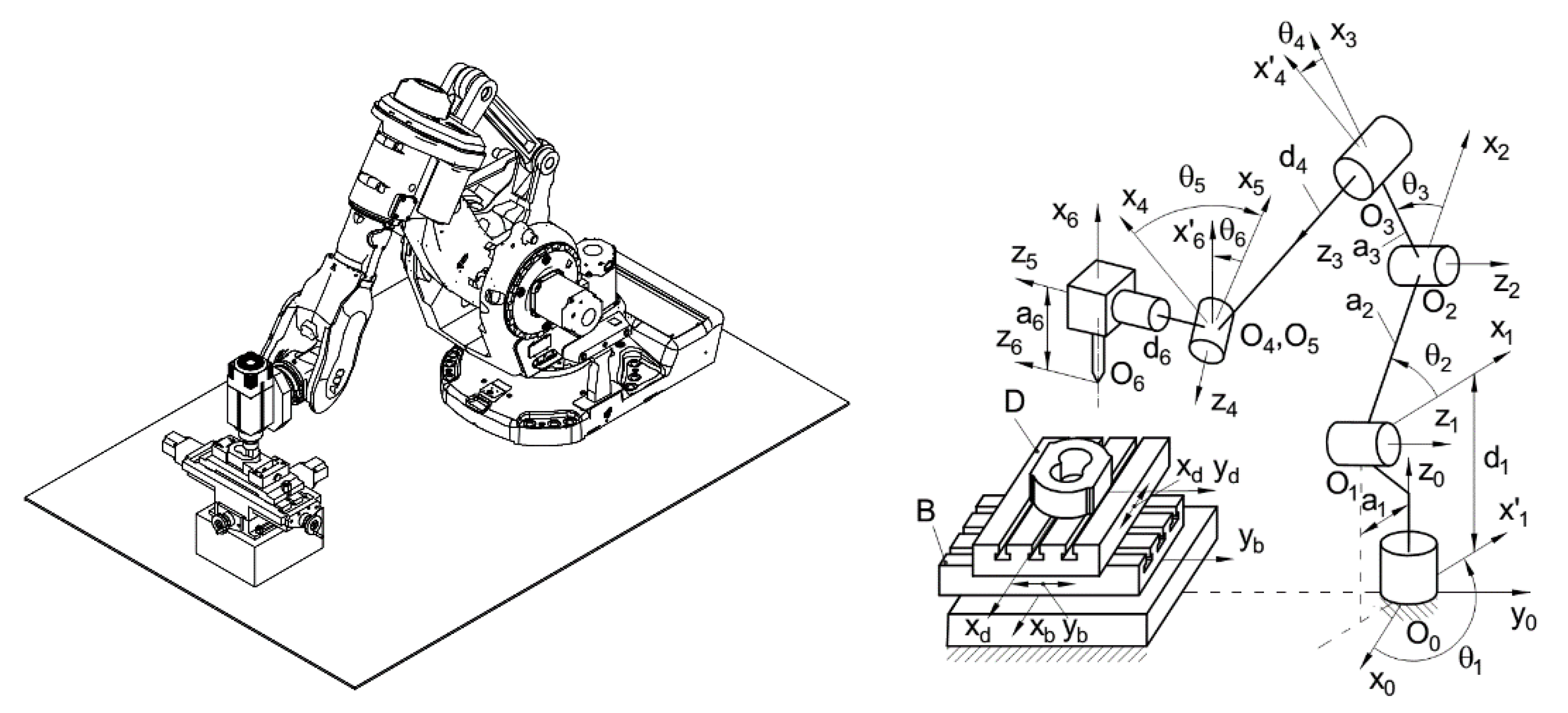
Figure 1. The model of robot; clamping platform has eight degrees of freedom (DOF) in milling process.
Applsci 10 01685 g001
Figure 2. Representation of the cutting force model of the cutting edge i of a disk dz in milling.
Applsci 10 01685 g002
Figure 3. Scheme of the inverse dynamics method combined with the law of derivative proportional control (Inverse Dynamics + PD) controller in joint space
Applsci 10 01685 g003
Figure 4. The membership function of position error, velocity error and adjustment amount of driving torque of joint i: yi (yi = ei, e ˙ i , ui; i = 1, …, 8).
Applsci 10 01685 g004
Figure 5. Scheme of fuzzy logic control for the robot–platform system in machining.
Applsci 10 01685 g005
Figure 6. General block diagram of fuzzy control.
Applsci 10 01685 g006
Figure 7. Block diagram of dual-loop fuzzy control.
Applsci 10 01685 g007
Figure 8. The workpiece and the tool path.
Applsci 10 01685 g008
Figure 9. The end mill cutter.
Applsci 10 01685 g009
Figure 10. The cutting forces corresponding to the two cases of calculation and cutting force coefficient selection. (a)Fx-(N);(b)-Fy(N); (c)Fz-(N);(d)-Mz(Nm).
Applsci 10 01685 g010
Figure 11. The errors of the joint positions of the PD1, PD2 controllers.
Applsci 10 01685 g011
Figure 12. The errors of the cutting trajectory with respect to the set one are the toolpaths of the PD1, PD2 controllers.
Applsci 10 01685 g012
Figure 13. The joint position errors of the PD1, PD2, fuzzy controllers.
Applsci 10 01685 g013aApplsci 10 01685 g013b
Figure 14. The errors of the cutting trajectory with respect to the set one are the toolpaths of the PD1, PD2, FZ controllers.
Applsci 10 01685 g014
Figure 15. The trajectory of the cutting point with respect to the operational frame. (a)- when there is no initial deviation; (b)- there is initial deviation.
Applsci 10 01685 g015
Figure 16. The simulation result of the fuzzy controller with initial trajectory error.
Applsci 10 01685 g016aApplsci 10 01685 g016b
Figure 17. Membership function value of the fuzzy set u(t) corresponding to the physical value domain of u(t) is selected as in Table 6.
Applsci 10 01685 g017
Figure 18. Membership function value of the fuzzy set u(t) corresponding to the physical value domain of u(t) is chosen to be 3 times larger than the value in Table 6.
Applsci 10 01685 g018
Figure 19. Tool path position errors between desired value and simulation result in normal cutting force mode.
Applsci 10 01685 g019
Figure 20. Tool path position errors between desired value and simulation result in cutting force mode increases by 50% due to noise.
Applsci 10 01685 g020
Table 1. The frames and homogeneous coordinate transformation matrices.
LinksFrameKin. Parameters i−1Ai0Ai
The robot kinematic chain
L0O0x0y0z00, …, 0EE
L1O1x1y1z1θ1, d1, a1, α10A11)0A11)
L6O6x6y6z6θ6, d6, a6, α65A66)0A11)... 5A66)
Cutting toolOExEyEzE6xE, 6yE, 6zE,
6αE, 6βE, 6ηE
6AE0A11)... 5A66)6AE
The platform kinematic chain
L0O0x0y0z00, …, 0EE
L0’O0’x0’y0’z0’x0’, y0’, z0’,
α0’, β 0’, η 0’
0A0’0A0’
BObxbybzbxb, yb, zb,
αb, β b, η b
0’Ab(yb)0A0’0’Ab(yb)
DOdxdydzdxd, yd, zd,
αd, β d, ηd
bAd(xd)0A0’0’Ab(yb) bAd(xd)
Cutting toolOExEyEzEdxE, dyE, dzE,
dαE, dβE, dηE
dAE0A0’0’Ab(yb) bAd(xd) dAE
Table 2. Description of physical domains, fuzzy set and linguistic values of the inputs and outputs.
Serial No.Physical Domain XjFuzzy Set FjName of Linguistic Value Notation of Linguistic Value
1X1F1Big NegativeNB
2X2F2Small NegativeNS
3X3F3ZeroZ
4X4F4Small PositivePS
5X5F5Big PositivePB
Table 3. Fuzzy rules.
Adjustment Velocity   Error   e ˙ ( t )
Amount u(t) NBNSZPSPB
Position error e(t)NBPBPBPBPSZ
NSPBPSPSZNS
ZPBPSZNSNB
PSPSZNSNSNB
PBZNSNBNBNB
Table 4. The cutter parameters and the milling process parameters.
Cutter’s MaterialD1 (mm)D2 (mm)L1 (mm)L2 (mm)Z (tooth)vc (m/min)vr (mm/s)Sz (mm/tooth)h0 (mm)Cooling Liquor
Carbide202012550431.33.30.12.2Emunxi
Table 5. Cutting force coefficients in milling.
CaseKtc (N/mm2)Krc (N/mm2)Kac (N/mm2)Kte (N/mm)Kre (N/mm)Kae (N/mm)
11825 77073529.755.71.8
21963 64677829.755.71.8
Table 6. The physical value domain of input and output quantities of the fuzzy controller.
Linkei e ˙ i ui
1[−0.001,0.001] (rad)[−0.5,0.5] (rad/s) [−18,000,18,000] (Nm)
2[−0.001,0.001] (rad)[−2.4,2.4] (rad/s) [−44,000,44,000] (Nm)
3[−0.006,0.006] (rad)[−2.5,2.5] (rad/s) [−42,000,42,000] (Nm)
4[−0.009,0.009] (rad)[−12.0,12.0] (rad/s) [−18,000,18,000] (Nm)
5[−0.008,0.008] (rad)[−7.0,7.0] (rad/s) [−9800,9800] (Nm)
6[−0.008,0.008] (rad)[−10.0,10.0] (rad/s) [−5200,5200] (Nm)
7[−0.001,0.001] (m)[−0.2,0.2] (m/s) [−4700,4700] (N)
8[−0.001,0.001] (m)[−0.5,0.5] (m/s) [−3100,3100] (N)