Nonlinear Optimal Control Law of Autonomous Unmanned Surface Vessels


Abstract
1. Introduction
2. Mathematical Model and Design Objective
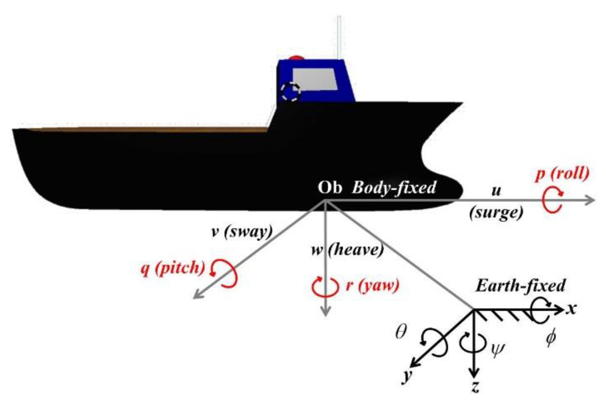
2.1. Rigid-Body AUSV Dynamics
2.2. Problem Formulation
2.3. Nonlinear Optimal Trajectory- and Waypoint-Tracking Problem of AUSVs
3. Results
3.1. Closed-form Solution of Nonlinear Time-Varying Differential Equation (13)
Closed-Form Solution of the Optimal Tracking Problem of AUSVs
3.2. Derivations of Optimal Parameters and for
4. Discussion
4.1. Parameterizations of Controlled AUSV and Ocean-Environment Disturbances
4.2. Control-Parameter Setup
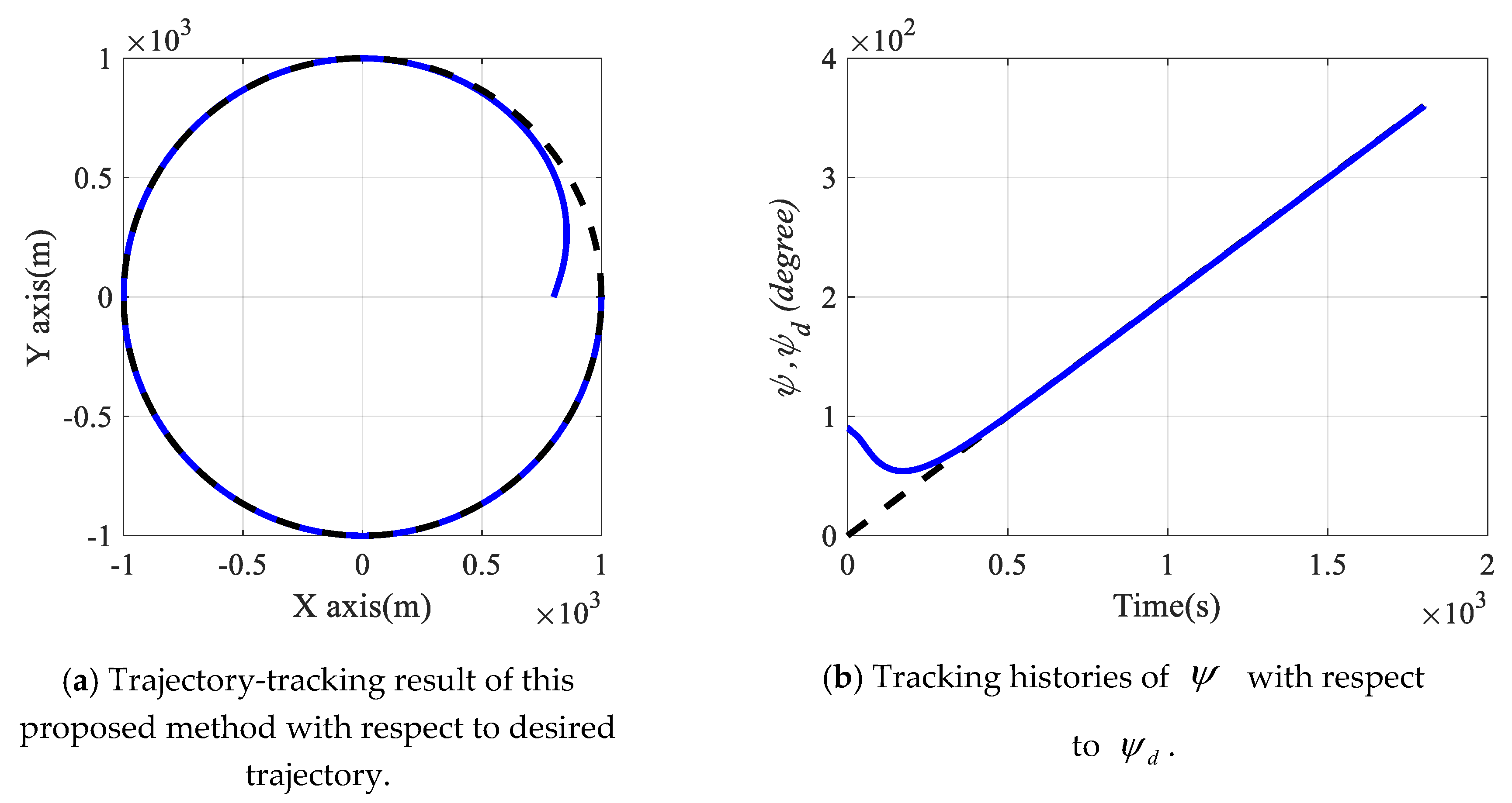
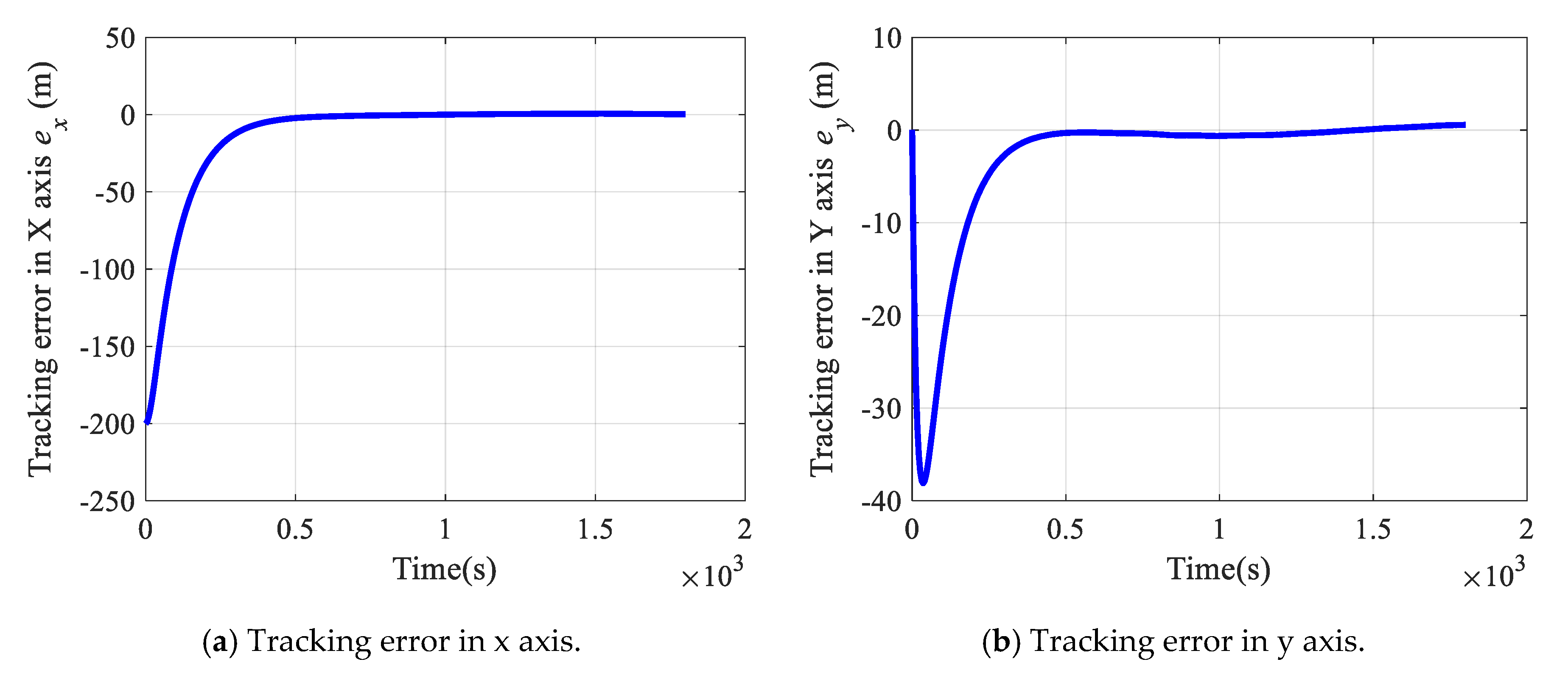
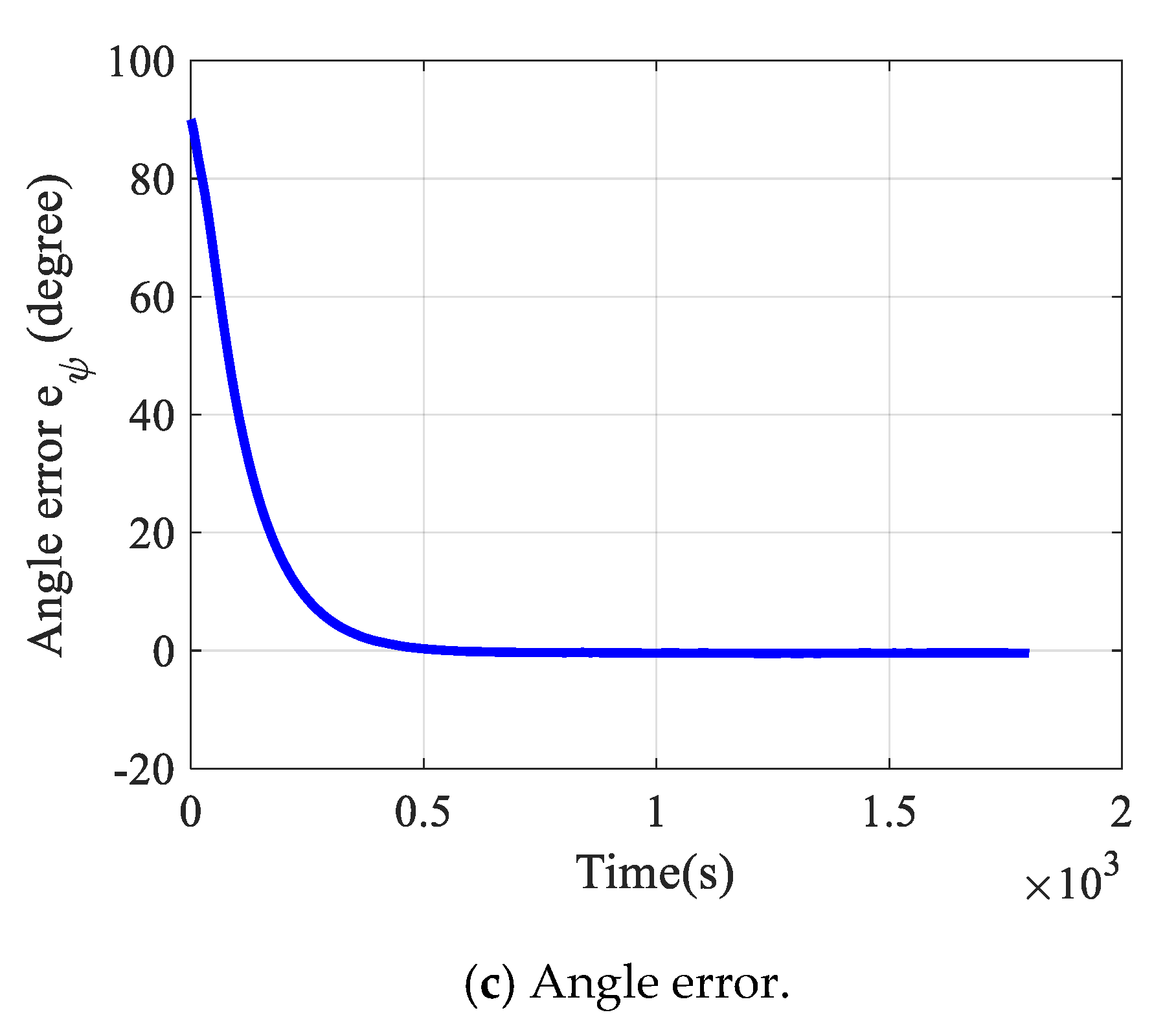
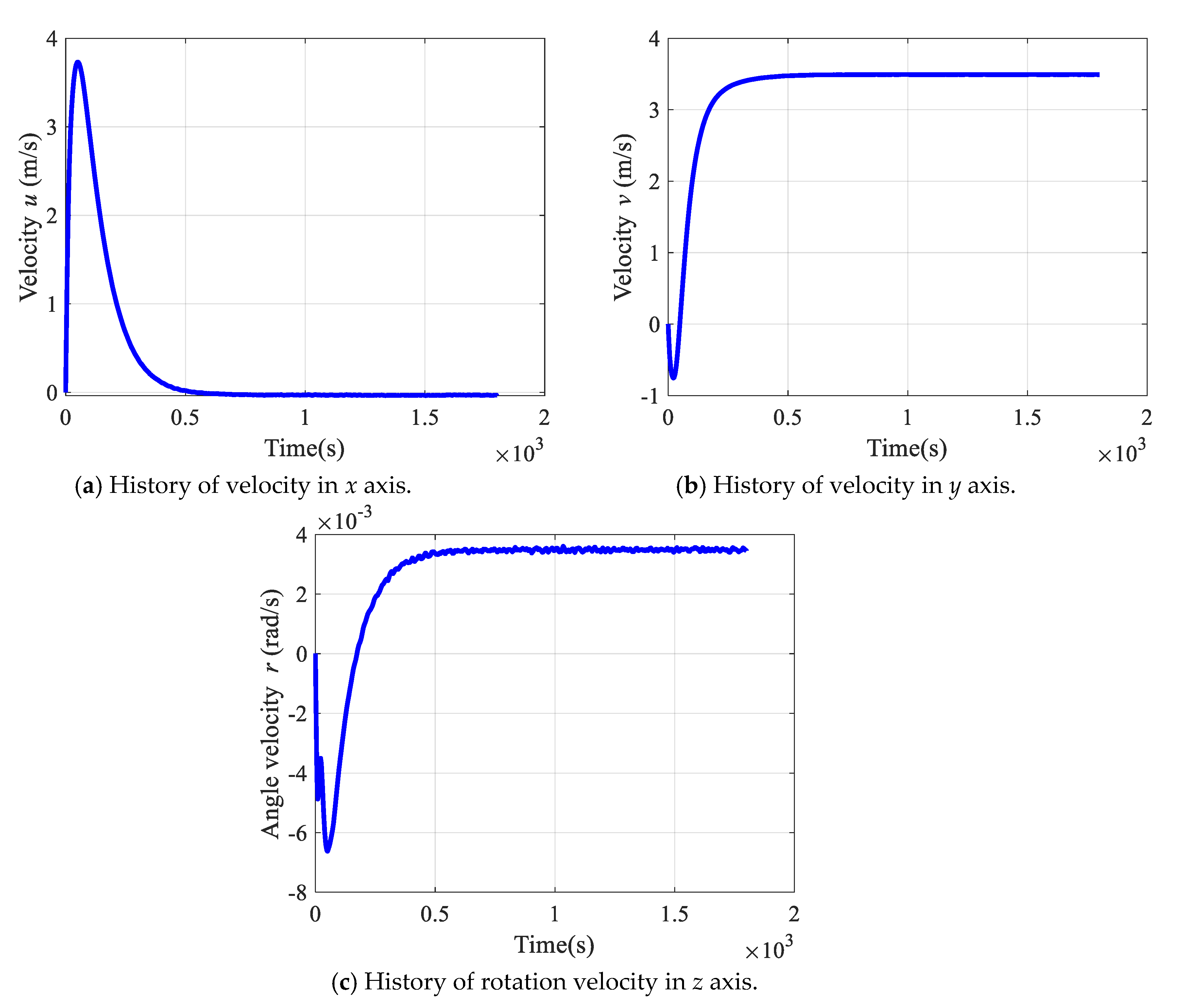
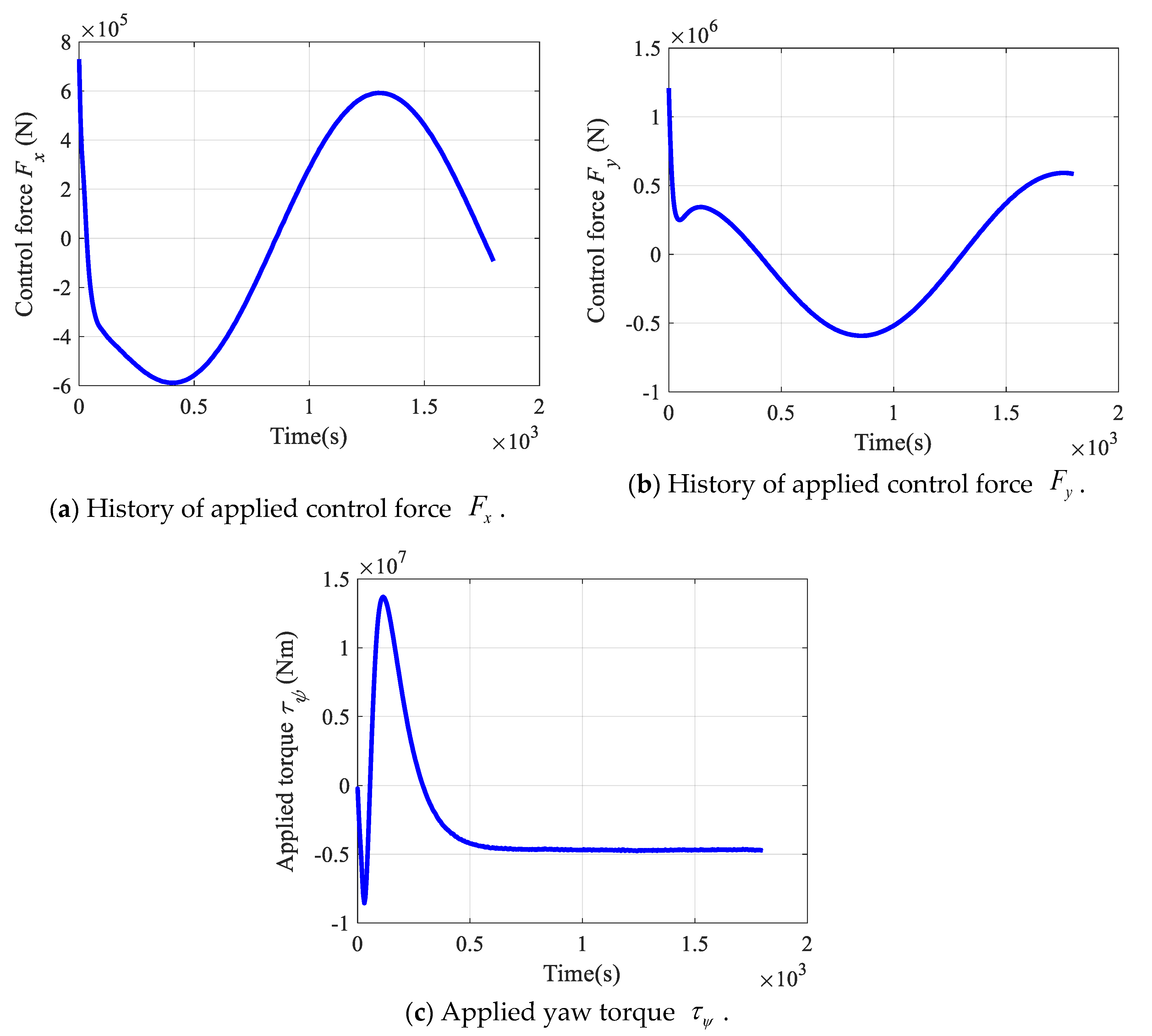
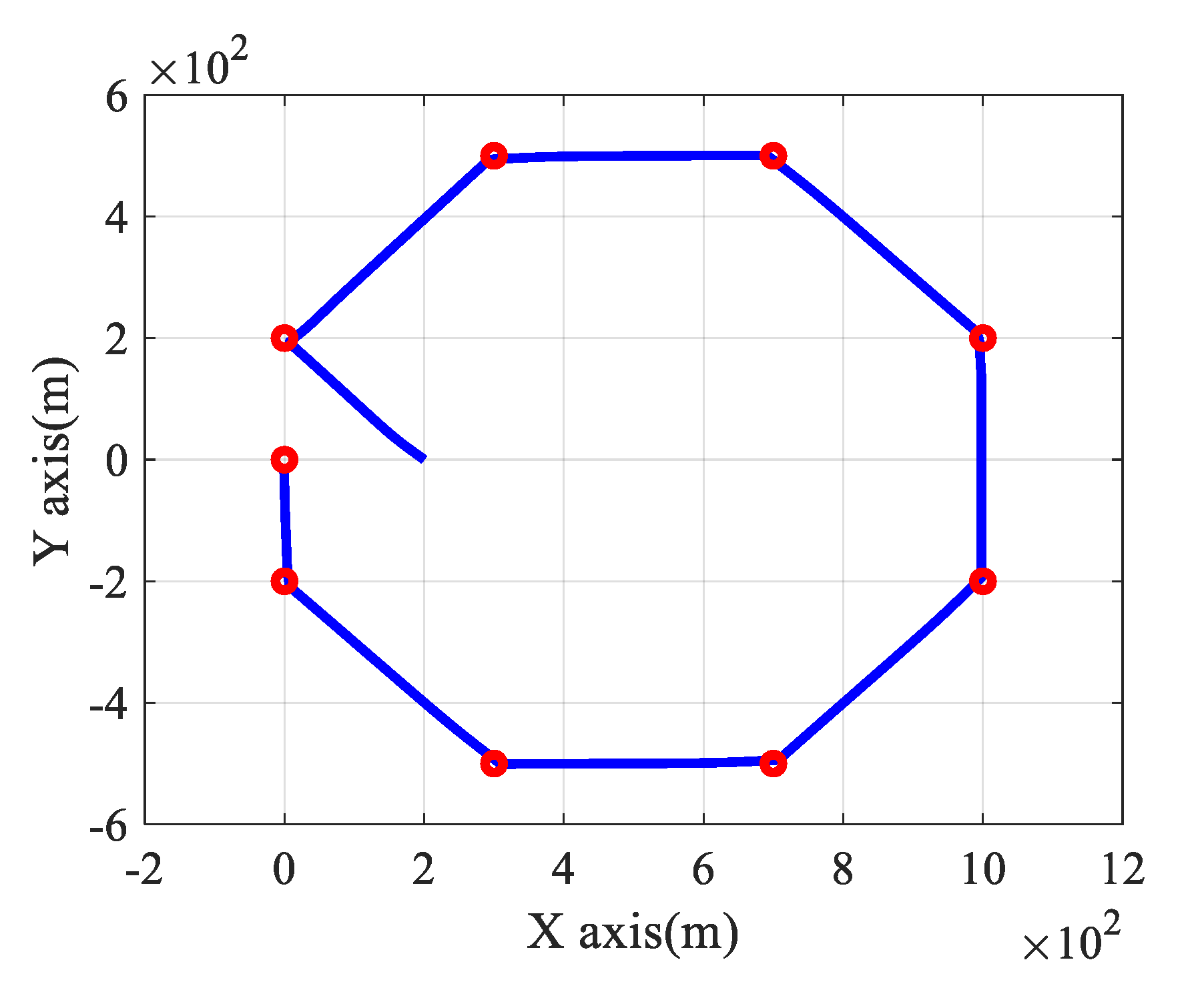
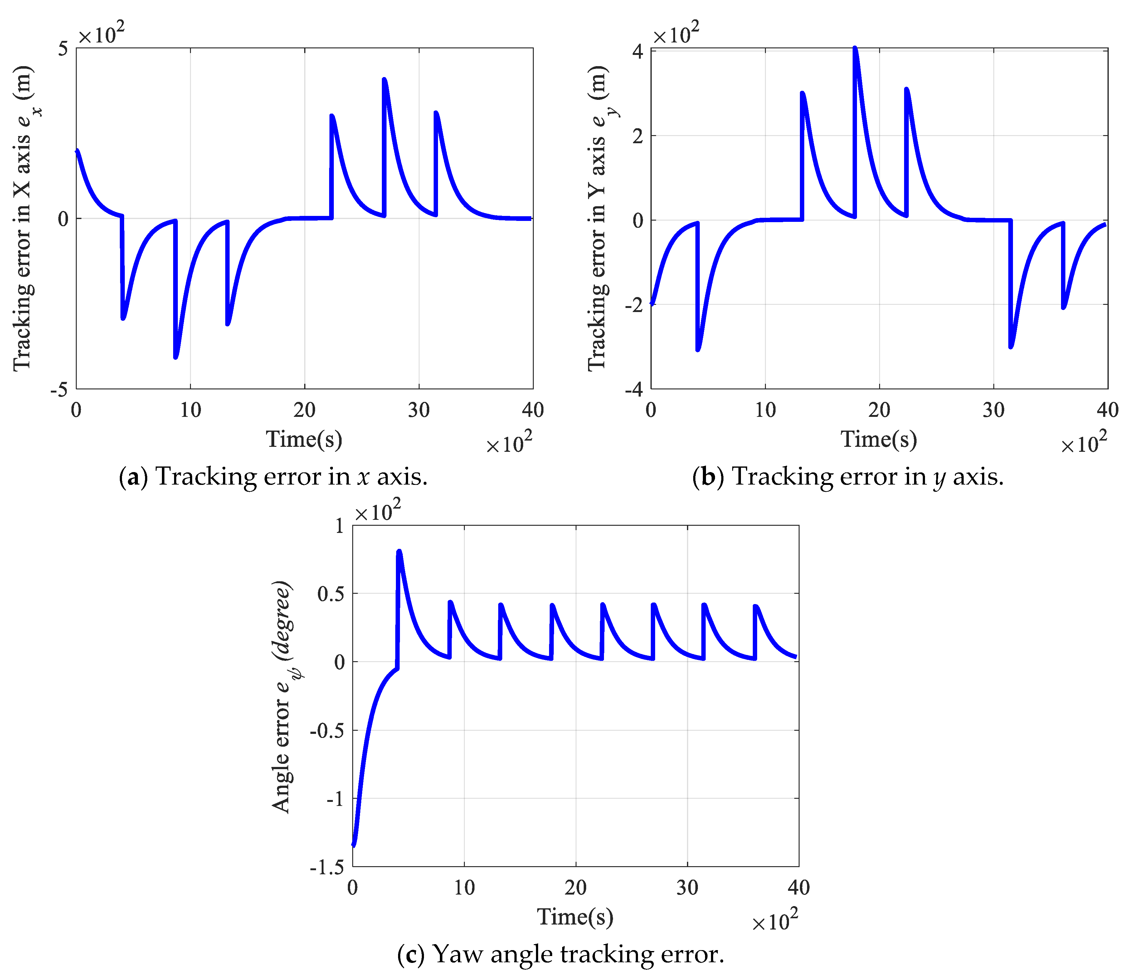
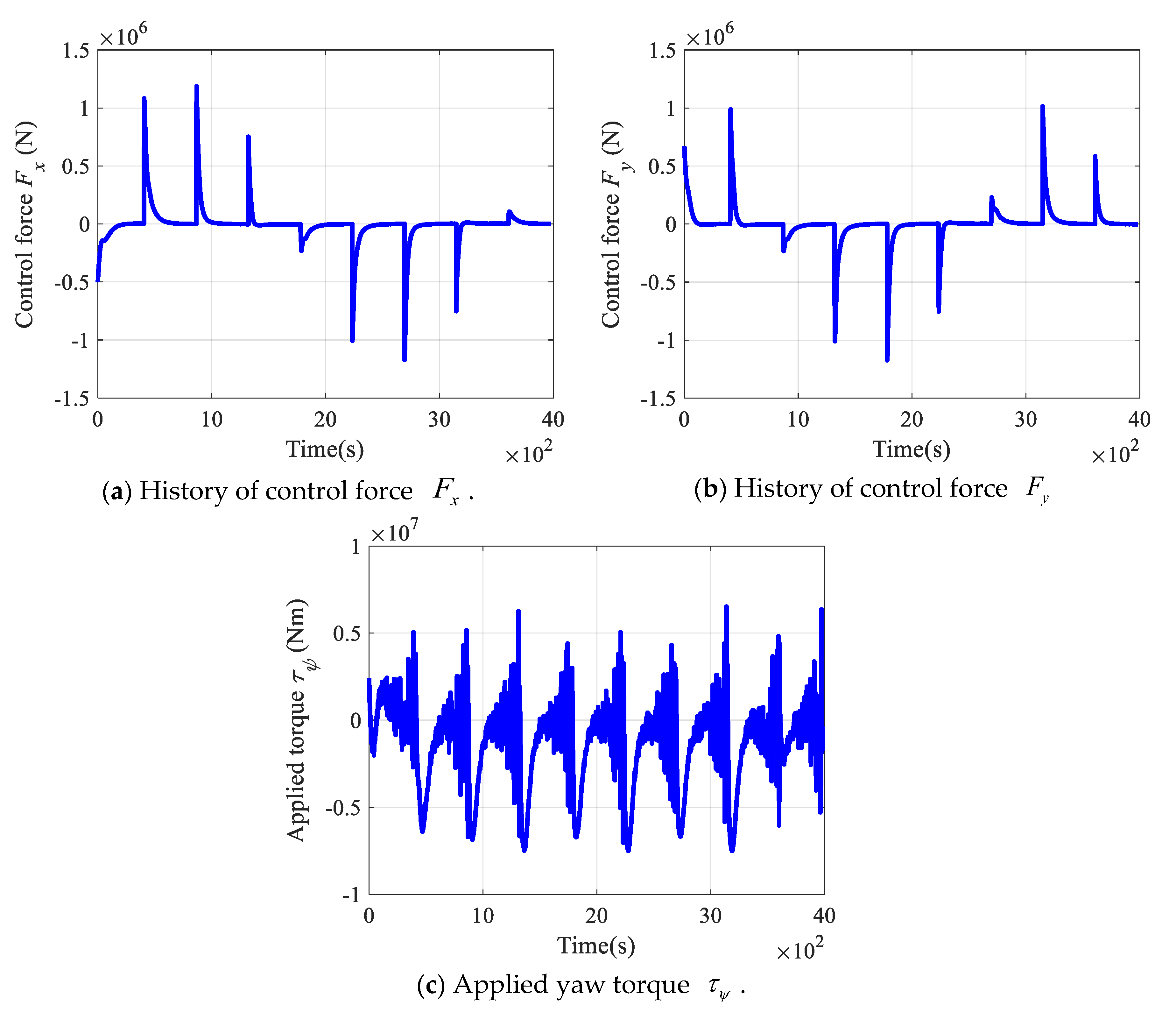
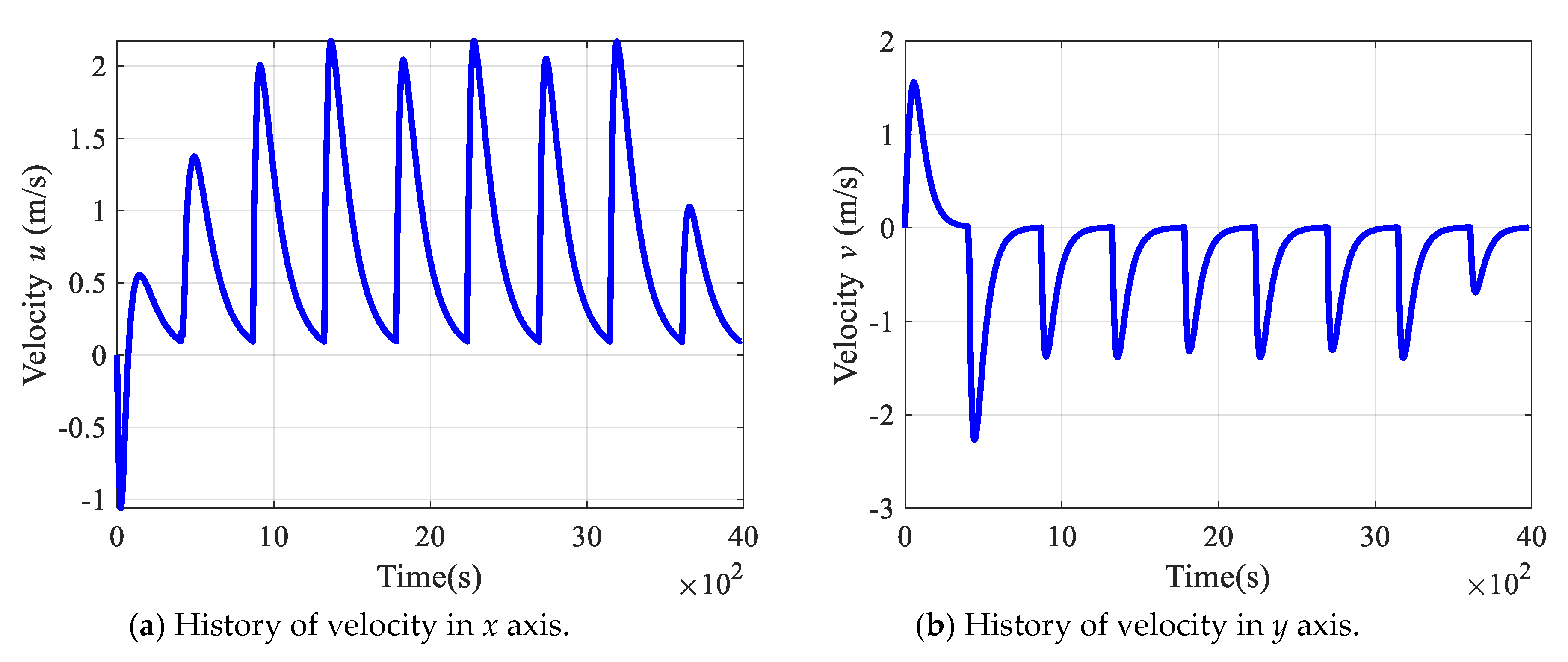
4.3. Simulation Results of Tracking Continuous Trajectory and Waypoints
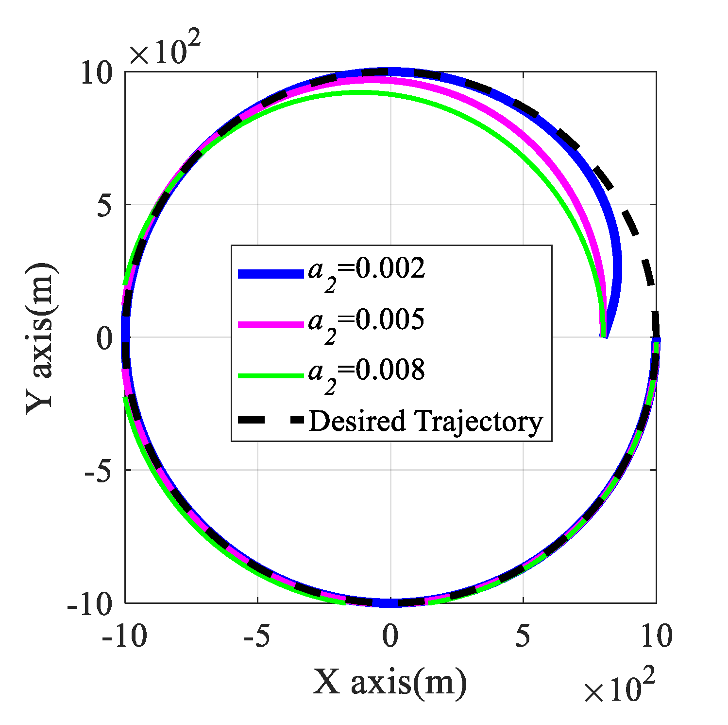
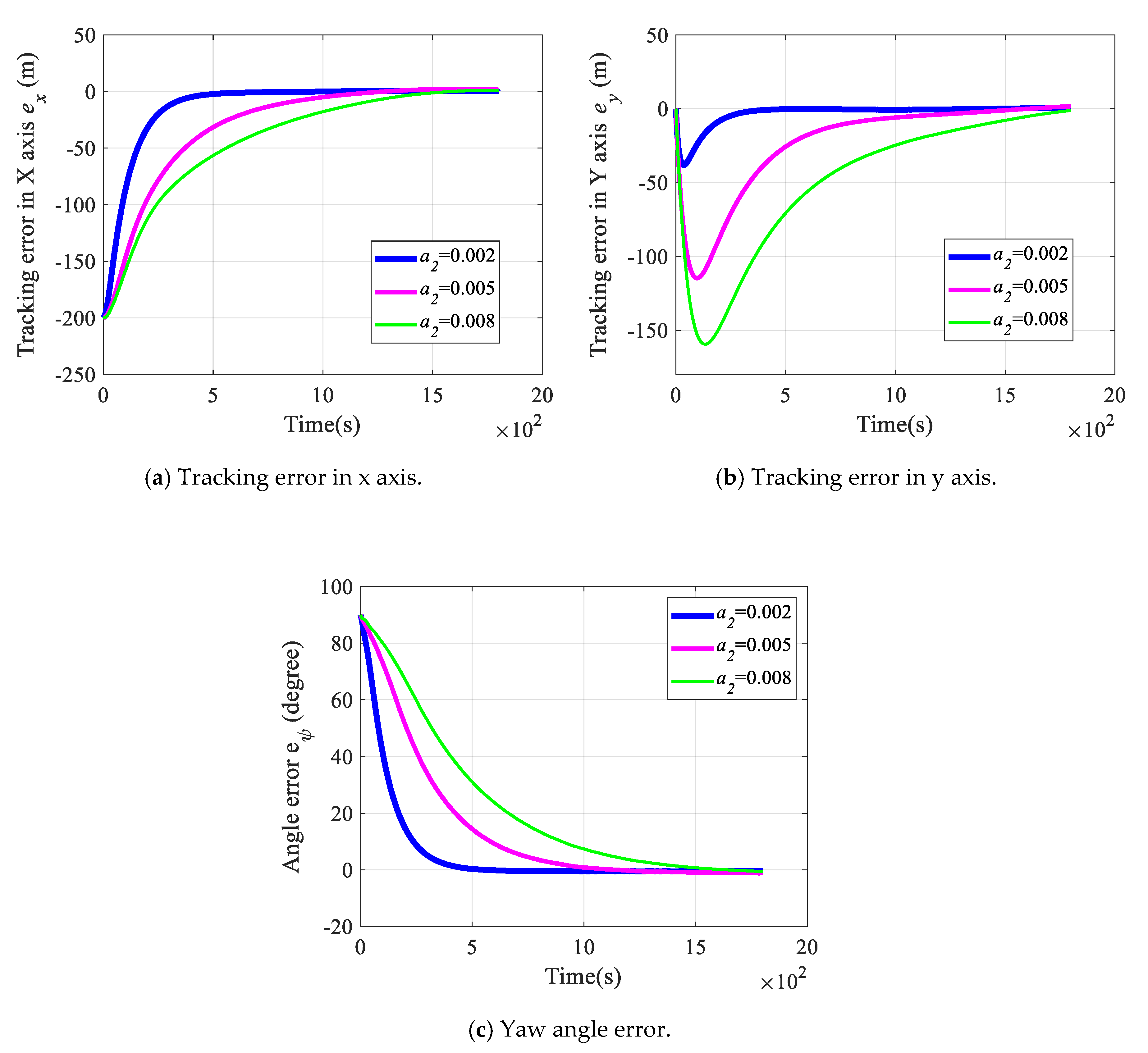
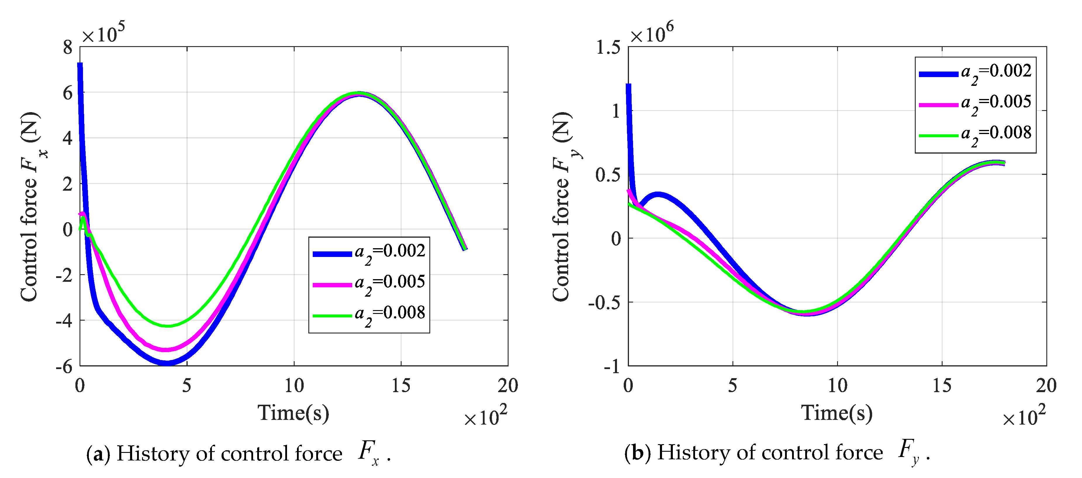
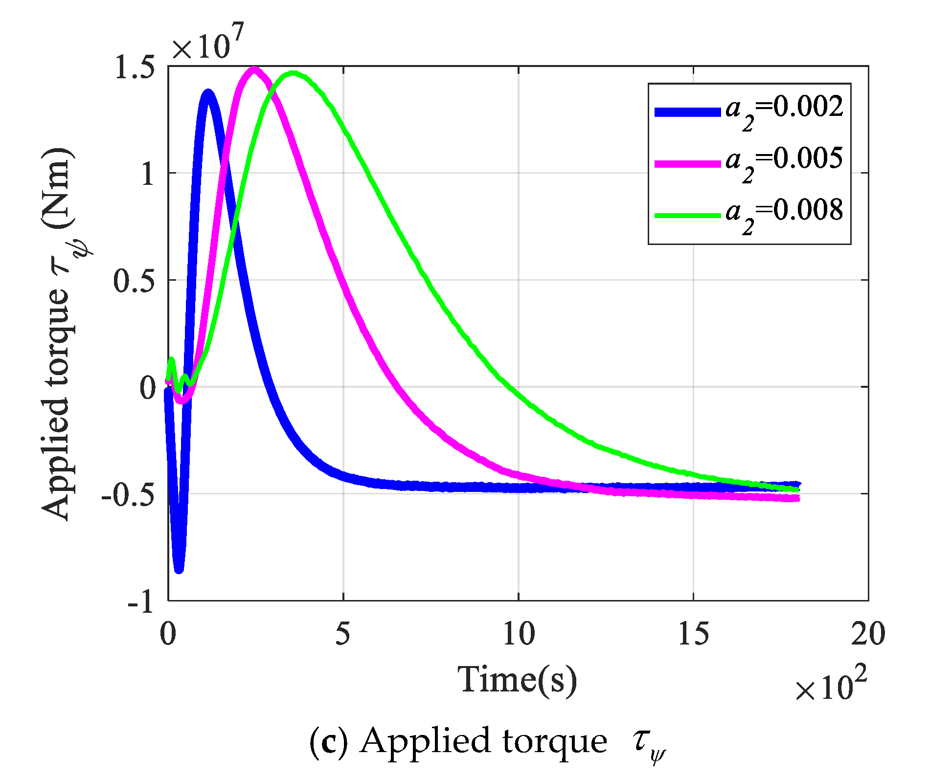
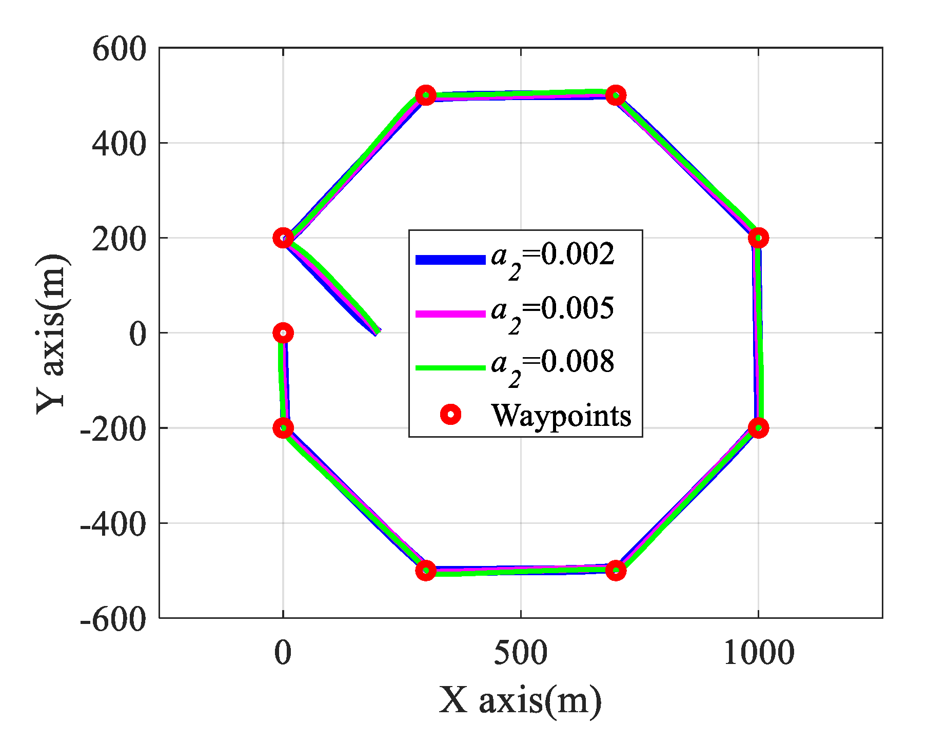
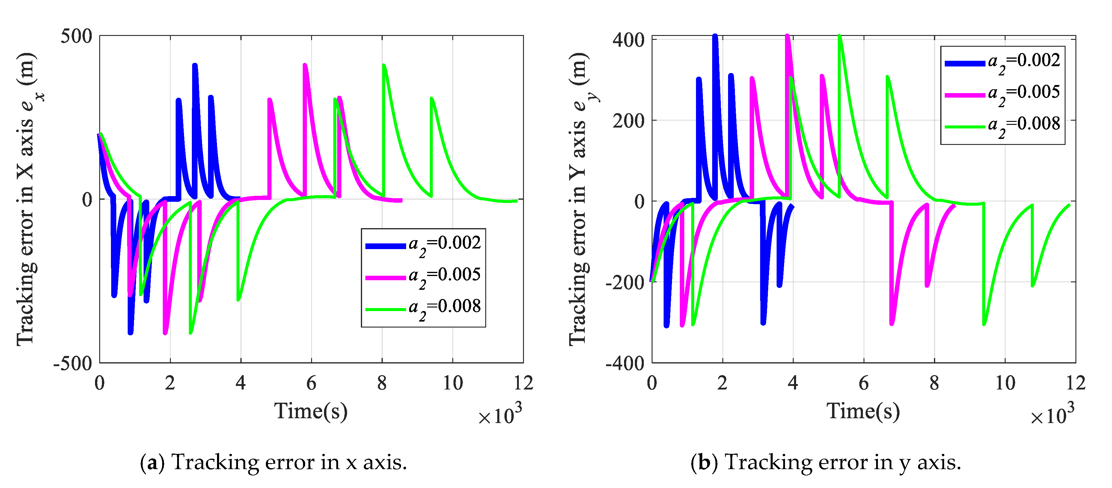
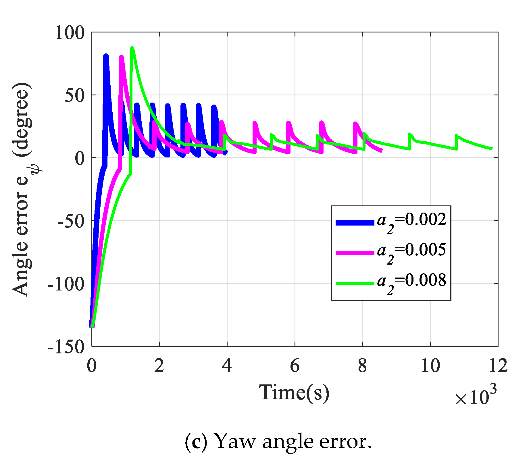
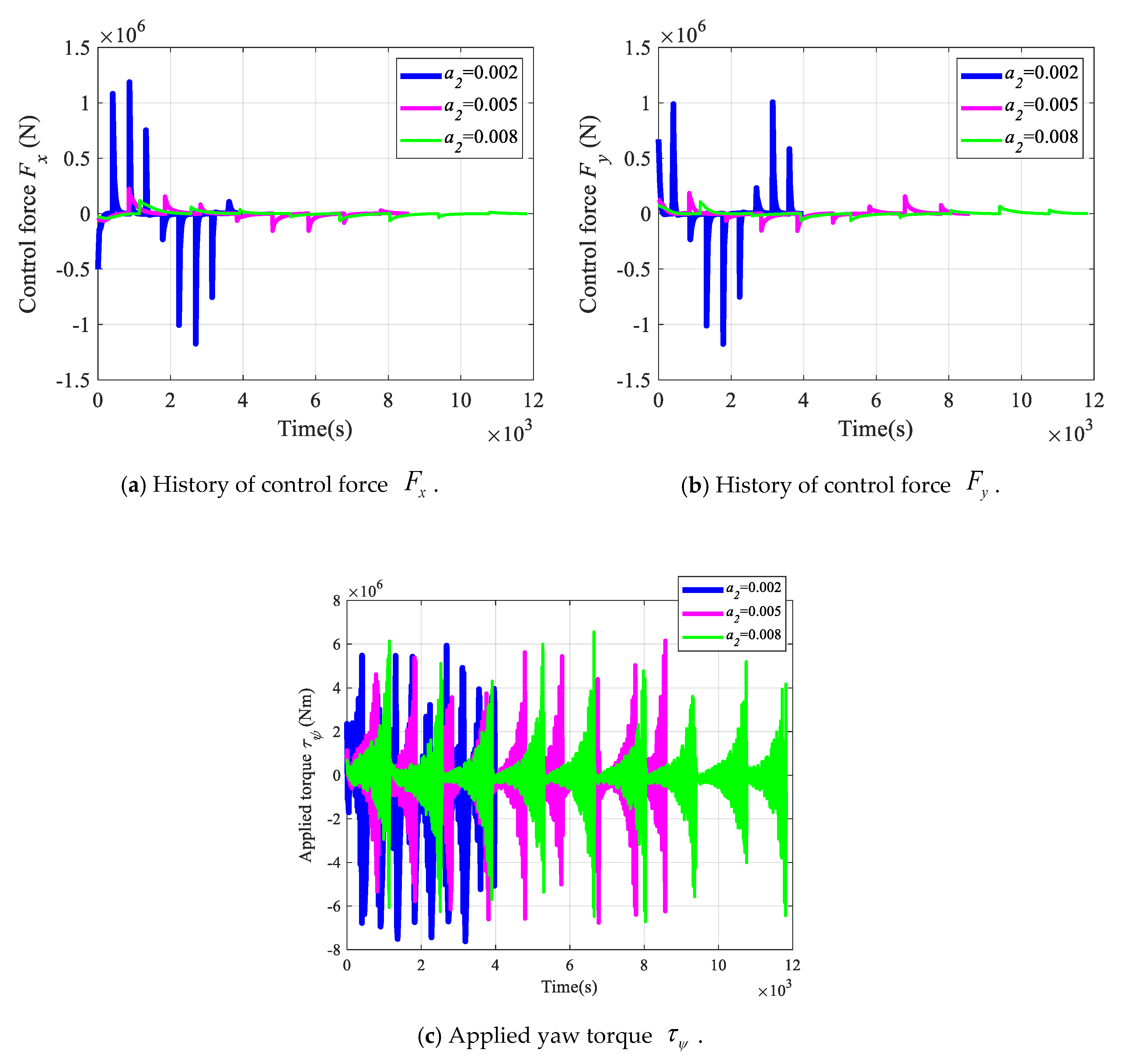
5. Comparisons of Tracking Performance with Respect to Different Control Gains:
6. Conclusions
Author Contributions
Funding
Conflicts of Interest
Appendix A
References
- Papoulias, F.A. Cross track error and proportional turning rate guidance of marine vehicles. J. Ship Res. 1994, 38, 123–132. [Google Scholar]
- Vukic, Z.; Ozbolt, H.; Pavlekovic, D. Improving fault handling in marine vehicle course-keeping systems. IEEE Proc. Robot. Autom. Mag. 1999, 6, 39–52. [Google Scholar] [CrossRef]
- Temel, T.; Ashrafiuon, H. Sliding-mode speed controller for tracking of underactuated surface vessels with extended Kalman filter. Electron. Lett. 2015, 51, 467–469. [Google Scholar] [CrossRef]
- Valenciaga, F. A second order sliding mode path following control for autonomous surface vessels. Asian J. Control 2014, 16, 1515–1521. [Google Scholar] [CrossRef]
- Kahveci, N.E.; Ioannou, P.A. Adaptive steering control for uncertain ship dynamics and stability analysis. Automatica 2013, 49, 685–697. [Google Scholar] [CrossRef]
- Qiaomei, S.; Guang, R. An online adaptive logic-oriented neural approach for tracking control. Ocean Eng. 2013, 58, 106–114. [Google Scholar] [CrossRef]
- Ghommam, J.; Mnif, F.; Derbel, N. Global stabilisation and tracking control of underactuated surface vessels. IEEE Control Theory Appl. 2010, 4, 71–88. [Google Scholar] [CrossRef]
- Chen, X.; Tan, W.W. Tracking control of surface vessels via fault-tolerant adaptive back stepping interval type-2 fuzzy control. Ocean Eng. 2013, 70, 97–109. [Google Scholar] [CrossRef]
- Serrano, M.E.; Godoy Bordes, S.A.; Gandolfo, D.; Mut, V.A.; Scaglia, G.J.E. Nonlinear Trajectory Tracking Control for Marine Vessels with Additive Uncertainties. Inf. Technol. Control 2018, 47, 118–130. [Google Scholar]
- Paliotta, C.; Lefeber, E.; Pettersen, K.Y.; Pinto, J.; Costa, M. Trajectory tracking and path following for underactuated marine vehicles. IEEE Trans. Control Syst. Technol. 2019, 27, 1423–1437. [Google Scholar] [CrossRef]
- Serrano, M.E.; Scaglia, G.; Godoy, S.A.; Mut, V.; Ortiz, O.A. Trajectory tracking of underactuated surface, vessels: A linear algebra approach. IEEE Trans. Control Syst. Technol. 2014, 22, 1103–1111. [Google Scholar] [CrossRef]
- Bertaska, I.R.; Shah, B.; von Ellenrieder, K.; Švec, P.; Klinger, W.; Sinisterra, A.J.; Dhanak, M.; Gupta, S.K. Experimental evaluation of automatically-generated behaviors for USV operations. Ocean Eng. 2015, 106, 496–514. [Google Scholar] [CrossRef]
- Fossen, T.I.; Sagatun, S.I.; Sorensen, A.J. Identification of dynamically positioned ships. Control Eng. Pract. 1996, 4, 369–376. [Google Scholar] [CrossRef]


| Parameter | Value | SI Unit |
|---|---|---|
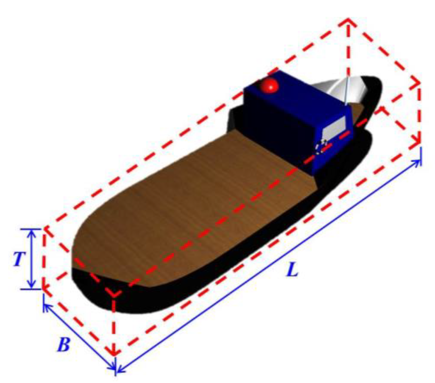
| Length (L) | 76.2 | m |
| Breadth (B) | 30 | m |
| Height (T) | 20 | m |
| Mass (m) | kg | |
| 0 | m |
| Parameter | Value | SI Unit |
|---|---|---|
| 2.0903 109 | kgm2 | |
| −0.5096 106 | kg | |
| −0.1698 106 | kg/s | |
| −3.5608 106 | kg | |
| 1.5081 106 | kgm/s | |
| −0.02268 109 | kgm | |
| 1.5081 106 | kgm/s | |
| −0.02268 109 | kgm | |
| −0.2530 109 | kgm2/s | |
| −0.8780 109 | kgm2 |
| Parameter | Value | Parameter | Value |
|---|---|---|---|
| Vω (m/s) | 3.96 | CXω(γR) | [−0.8 1] |
| CYω(γR) | [−0.7 1] | CNω(γR) | [−1.05 1.05] |
| ρair (kg/m3) | 1.1644 | ρω (kg/m3) | 1025 |
| g (m/s2) | 9.8 | N | 1000 |
| β | [−π π] | Ai | 3 |
| ϕi | [0 2π) | λi | 1 |
| Parameter | Value |
|---|---|
| 0.002 0.005 0.008 | |
| 0 | 0 | 1000 |
| 800 | 0 |
| Scenario 1: circular trajectory | Average run time: 2.6547 × 10⁻⁶ s. |
| Scenario 2: waypoints | Average run time: 2.0099 × 10⁻⁶ s. |
© 2020 by the authors. Licensee MDPI, Basel, Switzerland. This article is an open access article distributed under the terms and conditions of the Creative Commons Attribution (CC BY) license (http://creativecommons.org/licenses/by/4.0/).
Share and Cite
Chen, Y.-Y.; Lee, C.-Y.; Tseng, S.-H.; Hu, W.-M. Nonlinear Optimal Control Law of Autonomous Unmanned Surface Vessels. Appl. Sci. 2020, 10, 1686. https://doi.org/10.3390/app10051686
Chen Y-Y, Lee C-Y, Tseng S-H, Hu W-M. Nonlinear Optimal Control Law of Autonomous Unmanned Surface Vessels. Applied Sciences. 2020; 10(5):1686. https://doi.org/10.3390/app10051686
Chicago/Turabian StyleChen, Yung-Yue, Chun-Yen Lee, Shao-Han Tseng, and Wei-Min Hu. 2020. "Nonlinear Optimal Control Law of Autonomous Unmanned Surface Vessels" Applied Sciences 10, no. 5: 1686. https://doi.org/10.3390/app10051686
APA StyleChen, Y.-Y., Lee, C.-Y., Tseng, S.-H., & Hu, W.-M. (2020). Nonlinear Optimal Control Law of Autonomous Unmanned Surface Vessels. Applied Sciences, 10(5), 1686. https://doi.org/10.3390/app10051686