Article

Measurement and Modeling of 3D Solar Irradiance for Vehicle-Integrated Photovoltaic

1
Toyota Technological Institute, Nagoya 468-8511, Japan
2
Organization for Promotion of Tenure Track, University of Miyazaki, Miyazaki 889-2192, Japan
*
Author to whom correspondence should be addressed.
Appl. Sci. 2020, 10(3), 872; https://doi.org/10.3390/app10030872
Submission received: 2 January 2020 / Revised: 17 January 2020 / Accepted: 22 January 2020 / Published: 27 January 2020

Abstract

:

Featured Application

This technology is expected to be applied to vehicle-integrated photovoltaic.

Abstract

The energy yield of vehicle-integrated photovoltaics (VIPV) differs from that of standard photovoltaics (PV). It is mainly by the difference of the solar irradiance onto the car roof and car bodies as well as its curved shape. Both meaningful and practical modeling and measurement of solar irradiance for VIPV need to be established, rather than the extension of the current technologies. The solar irradiance is modeled by a random distribution of shading objects and car orientation with the correction of the curved surface of the PV modules. The measurement of the solar irradiance onto the car roof and car body is done using five pyranometers in five local axes on the car for one year. The measured dynamic solar irradiance onto the car body and car roof is used for validation of the solar irradiance model in the car.

1. Introduction

Let us think about a solar engine car, considering the recent development and success of EVs (electric vehicles) and PHVs (plug-in hybrid vehicles). Photovoltaic (PV) technologies will be game-changing in the automobile industry. It may be a dream now, but it is worth challenging [1].
The case study of the photovoltaic (PV) driven cars was conducted both by car manufacturers [2] and a think tank [3], and both reached the same conclusion in 2017. About 70% of a vehicle can run exclusively by solar energy on a different calculation basis [2,3]. The calculation base is published, namely: projected area of PV is 3.23 m2, temperature loss is 9%, Maximum power point tracking (MPPT) loss is 5%, DC-to-DC converter (DC is direct current) loss is 10%, battery charging and discharging loss is 5%, Electronic Control Unit (ECU) loss is 0.12 kWh/day, mileage is 12.5 km/kWh for electric vehicles (EVs), 10 km/kWh for plug-in hybrid vehicles (PHVs), and the battery size is 40 kWh to EVs and 10 kWh to PHVs. Then, the requirement of the car roof PV is 1 kW. As a result, 70% of cars (runs less than 30 km/day) are expected to run by solar energy [2,3,4]. When we multiply 71 million vehicles (annual sales in 2017), the expected sales are 50 GW/year (50,000,000 kW/year) [5]. The above calculations assume that the solar cells are stabilized with no or negligible degradation. However, some solar cells degrade with time, and this should be considered, in case such type of solar cells such as, amorphous Si [6], perovskite [7], crystalline Si [8], and Si module [9] are used. The photovoltaic is also useful for auxiliary powers and range-extension of other low-carbon energies, like hybrid vehicles [10], electric vehicles [11], as well as researches on innovation of the usage of solar energy [12] like, auxiliary power [13], charging [14], and support for fuel cells [15].
The efficiency and power rating, as well as energy prediction under the curved surface affected by the shading objects, are critical. For example, the car roof is three-dimensionally curved, and its curvature may induce power loss by increased cosine loss and self-shading loss [1]. This activity is mainly done by an international web-meeting which targets standardization of the vehicle-integrated photovoltaic and regularly publishes almost every half-year with the progress of arguments [16,17,18,19,20]. The irradiance and temperature of the car roof are different from that of the roof top or the ground mounting systems [16]. The expected energy yield should be different.
Car roofs are often shaded, resulting in significant losses by string mismatching [1]. It may be improved by the introduction of a power distribution circuit for compensating the mismatch in view of dynamic shading [21], alignment issue [22], and sampling interval [23]. However, due to the limited area and allowed thickness on the car roof, the most practical approach increases the number of series-connected strings [24].
Another aspect is that the car roof PV is not in the installation of the standard slope angle and orientation. The orientation of the car roof changes with time without correlation to the sun direction. Surrounding buildings and other objects (trees and signals) often shade PV panels, and the variety of the curved shapes has a complicated impact. Such interaction needs to be taken into account [1].
The development of meaningful testing and modeling methods is done by an international group using the web-meeting mentioned above [16,17,18,19,20]. The three dimensional (3D) model of photovoltaic power generation developed initially in the car roof PV, namely VIPV (vehicle integrated photovoltaic), can be extended to VIPV applications with curved PV using a flexible one.
This article covers the modeling and measurement of the solar irradiance of the car body for accurate, meaningful, and non-biased estimation of the energy yield of automobile mounting PV modules.

2. Model

With the progress of automotive technology, it helps to cover the limited power output of the car roof PV so that most private cars will be able to run by solar energy equipped with high-efficiency and 3D curved solar panels [1], and will overcome the loss mentioned above. To do so, the conventional IEC 60904 international standard series for PV electrical characterization, now focusing on 2D flat panels, needs to expand to 3D shaped PV modules [1]. We attempt to define 3D solar irradiation and rating to the 3D curved solar panels [24], either through an analytic approach [25] or numerical calculation based on Monte Carlo methods (ray-tracing simulation) [26]. We also consider the cross effect between the 3D curved surface of the PV module and 3D solar irradiance around the module [24].
The standard PV modules are installed to avoid shadows. However, the car roof PV is not orientated for the utilization of solar energy. The driver’s convenience often shades the PV. The relative orientation of the PV on the car to the sun position is not fixed but frequently changes by driving. The PV on the car body and the car roof is curved. It is often shaded by its surfaces. Therefore, the scale of performance is reconstructed.
The position and height of the shading objects are often difficult to predict. For predicting the total solar energy to a vehicle (either annual or monthly basis) in a specific area, not in a particular driving course, it is convenient to predict the shading influence using rough indicators of the roughness of the land. The value of the annual or monthly solar irradiance value in a specific area is valuable to predict the driving performance of vehicles mounting the PV panel.
We consider the following car-specific issues:
  • Greater chance of shading by objects around the car (trees and buildings)
  • Curved surface
  • The orientation angle randomly varies
  • Mismatching loss by partial shading

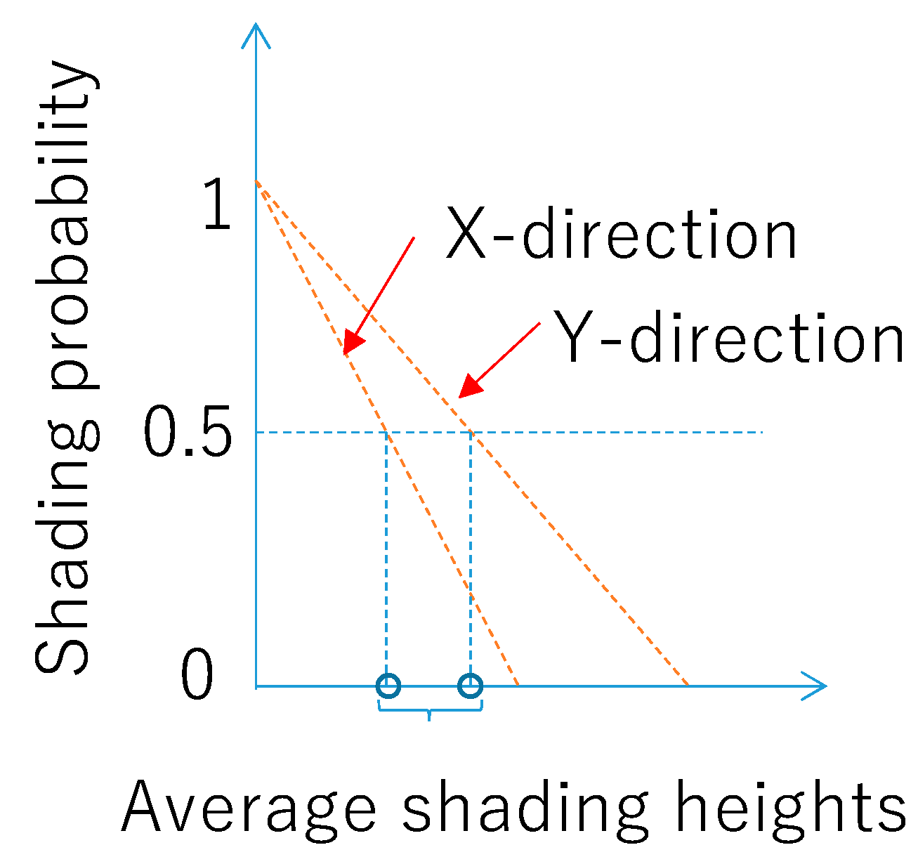
2.1. Shading Probability

The shading influence is complicated and varies by the position and the relative orientation (to the sun position) of the panel. In the case of the car roof PV, the position (orientation) of the panel cannot be predicted. One practical approach is to rely on the probability model, supposing that some statistical model randomly distributes the distribution of height and density of the shading objects, and the orientation of the car is independent and random as well.
Assuming that the segmented annular region, and the building or other shading objects are randomly distributed in this region with random height (Figure 1), the probability of the shading can be approximated as a linear relationship [26], because the height of the shading object is assumed to be inversely proportional to the distance from the car, whereas the number of shading objects along the arc of the given distance is proportional to the distance from the car so that the product of two factors is the constant value (Figure 2). Note that it is convenient to represent the height of the surrounding buildings and other shading objects scaling by the shading angle (grazing angle) [24].
Supposing the height of the shading object (represented by shading angle, namely, grazing angle) is distributed by the ranged uniform distribution, the accumulated distribution as a function of the shading angle (grazing angle) is calculated as a ranged integral so that the general trend is a linear one starting at zero degrees of the shading angle (grazing angle). It is also important to note that the distribution of the shading objects to the car and building is not axially symmetric and different in the direction parallel to the road and orthogonal to the road. Typically, the shading probability of the car roof PV along the road is less than that of the orthogonal direction of the road in the local coordinate. The area of the segmented annular is convenient to model such a situation (Figure 1) [24]. Note that the annular in place of the disk should be considered to avoid the situation of “division by zero” in angle calculation [26]. In addition, note that the line slope varies in two directions, one is along the road, and the other is orthogonal to the road [24]. A single parameter can represent this trend, namely, average shading height, corresponding to 50% probability of shading [26].

2.2. 3D Irradiance Model

For modeling the solar irradiance of the car roof, we assume a simple shading and scattering reflection model. The entire shading objects assume that the reflectance is 0.25, and the reflection is Lambertian. Both direct and scattered solar irradiance are assumed to be shaded by the shading objects as a function of the sun height and DNI (direct normal irradiance). The probability of the shading event calculates the shading probability and solid angle.
Assuming that the diffused irradiance from the unshaded sky is uniform, the factor of the diffused sunlight relative to the unshaded sky is approximated by the Equation (1) using random numbers. Note that the shape of buildings and other shading objects are rectangular, they are not spherical triangles or spherical trapezoids. It is realistic to model it as a cylinder sky using Equation (1).
σ s ( θ h ) = 1 ( 1 R b ) ( θ h 90 ° )
where σ s ( x ) is a function of the ratio of the diffused sunlight from the sky excluding the reflection of the direct sunlight to the shading objects, R b is the reflectance of the shading objects (fixed to 0.25 in this calculation), θ h is the average height of the shading objects scaled by the grazing angle (note that the maximum angle is 45° in this model).
The direct sunlight was approximated by Equation (2).
σ d ( η , θ h ) = [ 0 ( η < 0 ) η 2 θ h ( 0 η 2 θ h ) 1 ( η > 2 θ h )
where σ d ( x , y ) is a function of the ratio of illumination of the direct sunlight with the sun height x and the average shading height y .
The scattered sunlight by the reflection of the building from the direct sunlight is approximated by Equations (3) and (4). Note that the scattered irradiation by the reflection of the direct sunlight is seen on one side of the car body (not both sides), and the impact is half of the reflection by scattered light.
σ b s h ( η , θ h ) = 1 2 R b ( θ h 90 ° ) σ d ( η , θ h ) cos η
σ b s v ( η , θ h ) = 1 4 R b ( θ h 90 ° ) σ d ( η , θ h ) cos η
where σ b s h ( x , y ) and σ b s v ( x , y ) are functions of the ratio of illumination by the scattered reflection from the direct sunlight onto the horizontal and vertical planes with the sun height x and the average shading height y . Note that the illumination by the wall of the building happens on a single side of the road.
The directional cosine of the direct sunlight to the car side (vertical plane, random orientation) is approximated by Equation (5).
c θ s i d e ( ω ) = 0 ° 360 ° cos ( γ α ( ω ) ) ( cos ( γ α ( ω ) ) > 0 ) d γ 360 ° cos ( η ( ω ) )
where c θ s i d e ( ω ) is a function of the directional cosine of the direct sunlight to the car body as a function of the hour angle ω . The sun height η and the azimuth angle α are also the functions of ω . This equation also contains Boolean algebra in the parentheses that return 1 when the conditional equation is true and 0 when the conditional equation is false. Note that the azimuth angle is not needed to be considered in the calculation on the irradiance on the car roof (horizontal plane).
The irradiance on the car roof is approximated using the direct normal irradiance DNI and diffused irradiance from the sky SI using Equation (6) with calculation results of Equations (1)–(3).
C I r o o f = · σ s · S I + ( σ d sin η + σ bsh ) · D N I
where C I r o o f is solar irradiance onto the car roof affected by surrounding shades. Note that the arguments of functions in Equation (6) are omitted.
The irradiance on both car sides (both the direction parallel to the road and orthogonal to the road) is approximated by Equation (7) using Equations (1), (2), and (4)–(6).
C I s i d e = R r 2 C I r o o f + σ s 2 · S I + ( σ d · c θ s i d e + σ b s v ) · D N I
where C I s i d e is the solar irradiance onto the car side affected by surrounding shades, and R r is a reflection of the road. Note that the arguments of functions in Equation (7) are omitted as well.

2.3. Relation to the Conventional Solar Irradiance Model

For a definition of the angle of the solar irradiance and module orientation, the reference axis should be local to the automobile [1]. Each axis moves by the movement of the vehicle, and is independent of the orientation of the sun. On the other hand, the relative position is unchanged, and thus a linear coordinate conversion dynamically synchronized to the location, direction, and speed of the car, monitored by a GPS, handles this situation. The coordinate is an orthogonal one (Figure 3).
Supposing that the orientation of the car is independent of the sun’s position and random, the standard and local irradiance parameters of the car body can be converted to the following nine equations [1]. Some functions and equations contain Boolean algebra, and they return one or zero depending on whether the operation results are true or false. The vehicle body was always assumed as level.
Q r o o f = Q Z
Q s i d e = Q X + + Q X + Q Y + + Q Y 4
Φ = if ( Q Z > Q t h , tan 1 ( | max ( Q X + , Q X ) max ( Q Y + , Q Y ) | Q Z ) , N a N )
D = if ( min ( Q X + , Q X ) + min ( Q Y + , Q Y ) < Q s i d e , Q Z > Q t h , 0 )
where Qroof is the irradiance onto the car roof. Qside is the averaged irradiance of the car sides. Since the orientation of the car is independent of the sun’s orientation, the side irradiation may be regarded as the averaged value from four car sides. Φ is the main angle of the solar beam onto the car roof. Qth is the threshold of the effective measurement value of the irradiance. It must be greater than zero (non-zero value). NaN represents a missing or faulted value. D is the discriminant of the non-shaded condition. False (= 0) if the car roof is shaded. The function if(condition, x, y) returns x if the condition is true (non-zero), y otherwise. The function max(A, B, C, ...) returns the largest value from A, B, C, ... The function min(A, B, C, ...) returns the smallest value from A, B, C, ... Note that Equation (10) contains a two-dimensional vector calculation, and Equation (11) contains the Boolean algebra.
The orientation angle of the principal solar beam, not always equal to the orientation angle of the direct beam, is calculated by the following equations.
Q S 1 = max ( Q X + , Q X , Q Y + , Q Y )
Q S 2 = max 2 nd ( Q X + , Q X , Q Y + , Q Y )
a x 1 = ( Q S 1 = Q X + ) π 2 + ( Q S 1 = Q Y ) π + ( Q S 1 = Q X ) 3 π 2
a x 2 = ( Q S 2 = Q X + ) π 2 + ( Q S 2 = Q Y ) π + ( Q S 2 = Q X ) 3 π 2
G = m o d ( if ( ( Q S 1 > Q t h s ) ( | a x 1 a x 2 | = π 2 ) , tan - 1 ( Q S 2 Q S 1 ) s ign ( a x 2 a x 1 ) + a x 1 + D i r , N a N ) , 2 π )
where Qs1, Qs2, ax1, and ax2 are parameters calculated by Equations (12)–(15) and are used in Equation (16). G is the orientation angle of the main solar beam. Dir is the orientation angle of the car. The function max2nd(A, B, C, ...) returns the second largest value from A, B, C, ... The function mod(x, y) returns the remainder on dividing x by y (x modulo y). The result has the same sign as x. The function sign(x) returns 0 if x = 0, 1 if x > 0, and −1 otherwise. Note that Equations (14)–(16) contain Boolean algebra.
Mounting five orthogonally-arranged pyranometers, and applying Equations (8)–(16) to the monitored irradiance data, the three-dimensional solar irradiance around the vehicle may be modeled [27].

2.4. Angular Distribution Model

The angular distribution of the solar irradiance is calculated by the weighted histogram of the angular distribution. The angular distribution model is crucial both to the validation of the 3D solar irradiance model around the car body and optimization design of the high-performance static concentrator module (CPV) on the car roof [2]. For example, a new type of static concentrators consists of an array of dielectric lenses [28], its optimization algorithm for VIPV [29], combination to high-efficiency on Si tandem solar cells enhanced by an innovative partial concentrator configuration [30], its prototype [31], and demonstration to VIPV application [32]. In case the high-efficiency multi-junction cells are used for VIPV, it is essential to consider the spectrum impact correctly of the cross effect between the spectrum and angular distribution of the solar irradiance [33]. For example, a detailed spectrum energy model for the tandem solar cell was developed at the University of Miyazaki and recently published [34]. The model, as mentioned above, was expanded to the design of the future high-efficiency solar cell for VIPV application in the worst-case combination of atmospheric parameters [35] and realistic atmospheric parameters and measured spectrum [36]. The atmospheric parameters that impact performance of high-efficiency solar cells are identified using a statistical approach [37] and also to concentrator photovoltaic (CPV) [38] that is recently considered as a right candidate [39], fine-tuning of the bandgap design for VIPV application based-on the model as mentioned above [40], prediction of the energy yield with consideration of the spectrum and angular issues [41], and the rating method of the VIPV with consideration of above issues [42]. The detailed information of the high-efficiency PV modules used for the validation of the model is found in the article by Ota [43]. The angular distribution model is also useful for this purpose, but it is essential to note that it is deeply coupled with the spectrum variation that is not covered by this article. For the application of the angular model to the spectrum-sensitive tandem cells or CPV, it is indispensable to develop the 3D solar irradiation model further.
The meteorological data and irradiance data are given by the solar irradiance database, specifically, families of MEteorological Test data for PhotoVoltaic system (METPV), specifically, METPV-3 [44], METPV-11 [45], and METPV-ASIA [46]. It provides both direct and diffused irradiance every hour. The discrete sampling also makes the distribution shaggy, and to make it continuous, the event time is shifted in the range of plus or minus 30 min, also given by the random number under the ranged uniform distribution. The variance of the reflectance by the road and buildings (or mountains, etc.) also fluctuates the direction of the leading solar beam to the car. The modulation of the reflectance is also given by the random number, precisely, 0.10 to 0.40 for vertical reflection (building or trees), and 0.00 to 0.14 for the horizontal reflection (road).
However, the measurement system defined in Figure 3 does not have enough angular resolution. Instead, the measurement of the incident angle of the main beam is done by the ratio of the vertical irradiance (car roof) and the highest two irradiances of the car side, specifically, in Equation (10). The validation of the model in the angular distribution in this article is done by comparison of the weighted histogram of the main beam of the solar irradiance using Equation (10).

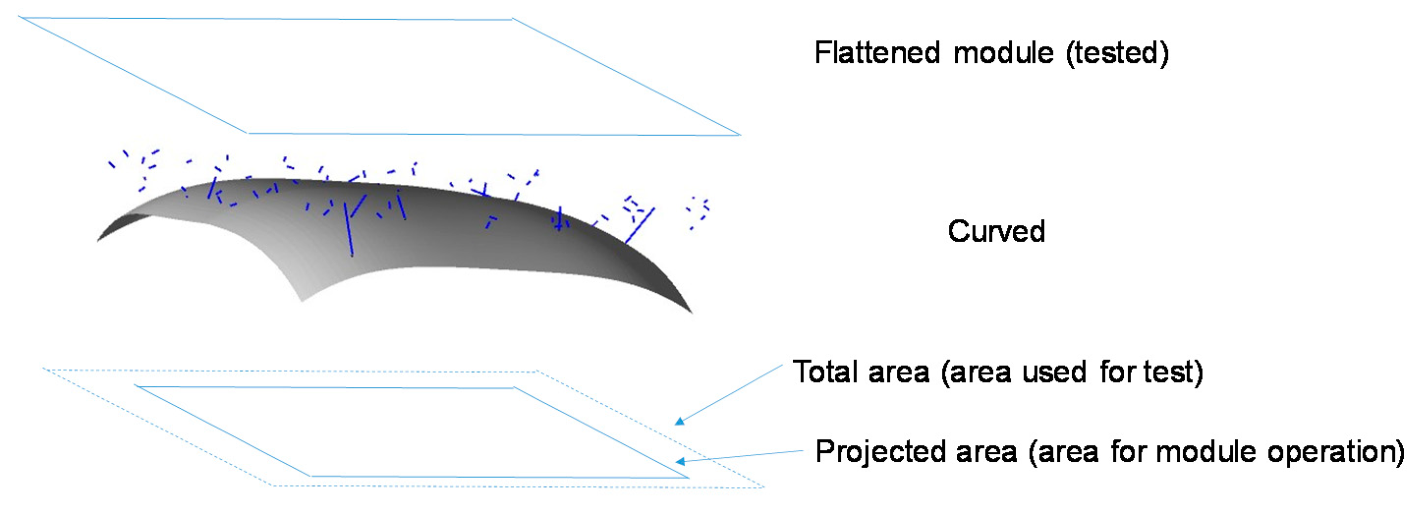
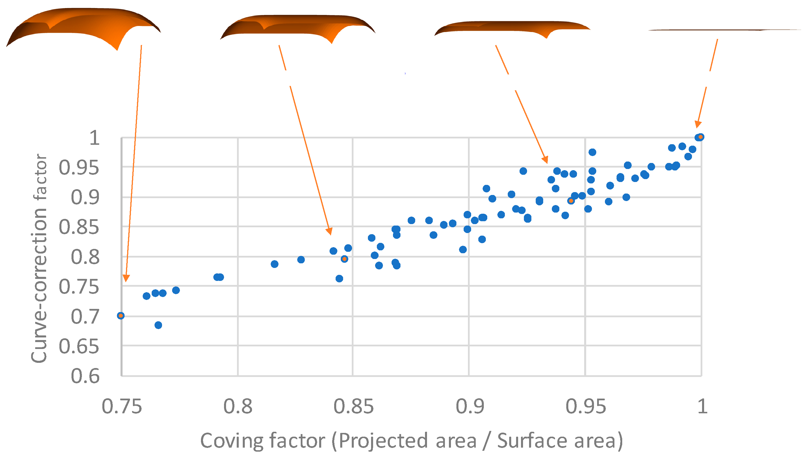
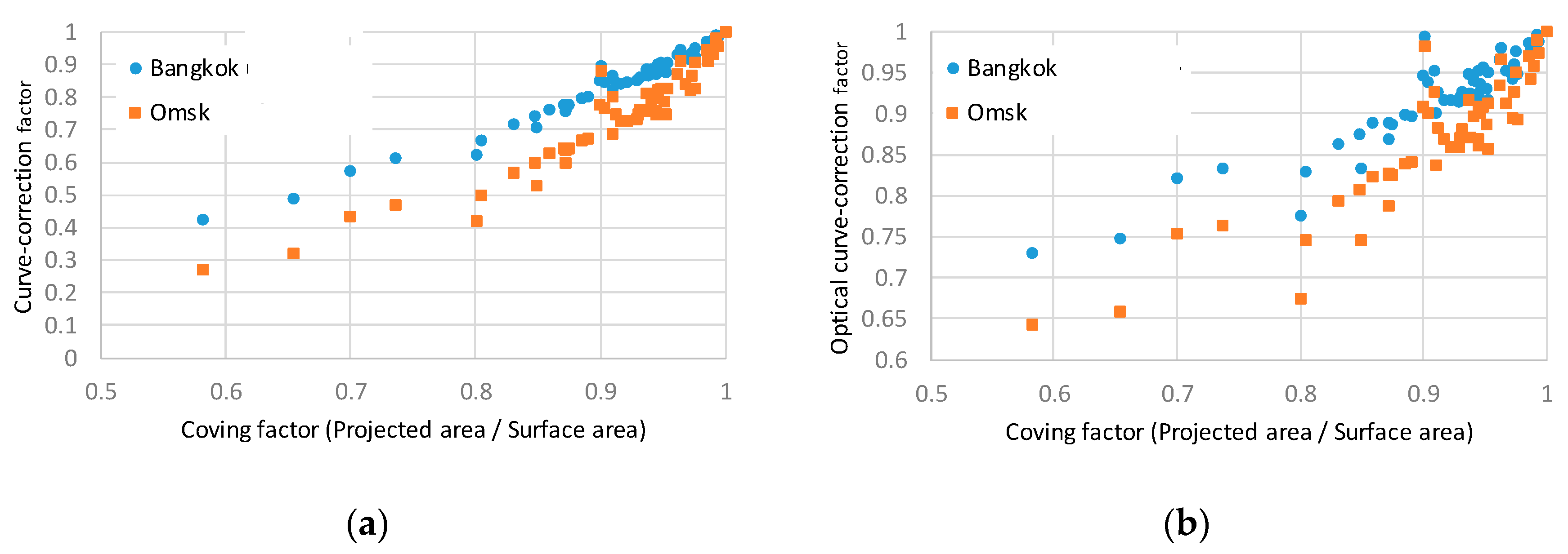
2.5. Curve Correction Model

All the formulas and protocols for measurement of the performance of the PV module is based on the preconditions that the PV modules are flat. For example, determination of the output power and other fundamental electrical parameters such as short-circuit current and open-circuit voltage of the PV modules, are essential to determine the input solar energy to the product of the irradiance and aperture area. On the other hand, the definition of the aperture area for the curved PV is not identical to the surface of the module. The car roof is three-dimensionally curved, and its curvature may induce power loss by increased cosine loss and self-shading loss [1]. Another aspect that we need to consider is that the car roof PV and BIPV (building integrated photovoltaic) are not in the installation of the standard slope angle and orientation. The orientation of the car roof changes with time without correlation to the sun direction. Surrounded buildings and other objects often shade both. These factors have a different impact on the curve shape. Such interaction needs to be taken into account.
We attempt to introduce a simple correction factor that includes complete irradiation loss to the curved surface. We call it the “curve correction factor.”

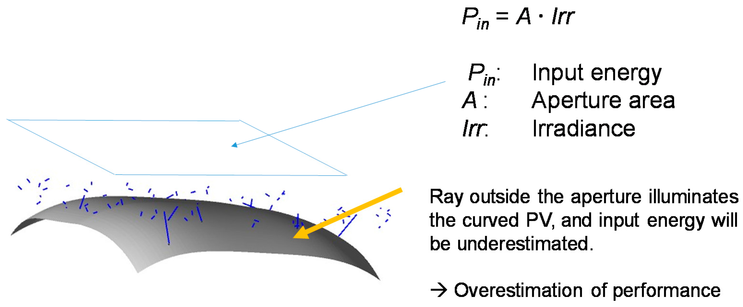
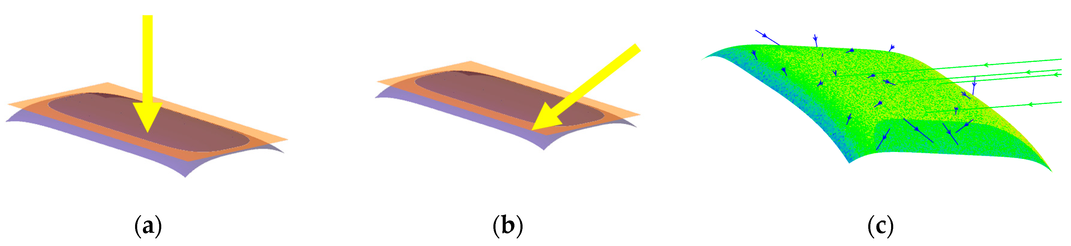
2.5.1. Why the Curved PV Modules are Often Overestimated in Efficiency Measurements

Before discussing the curve correction, let us clarify where the standard measurement method has a problem. The curved modules are often overestimated in efficiency measurements. It is because the input energy is often underestimated during the measurement by the indoor solar simulator.
To explain this, let us return to the definition of efficiency measurement of the solar cells and modules (Equation (17)).
η = P i n P o u t
where η is the measured energy efficiency of the solar cell or module using the solar simulator. P i n is the input power to the solar cell or the module. P o u t is the output power of the solar cell or the module. The measurement of P o u t of the curved module is the same as the standard flat PV modules, and it is a simple electrical measurement. However, the trappy measurement is P i n .
In the standard measurement of the solar cell and module, P i n is calculated by Equation (18).
P i n = A · I r r
where A is an aperture area. I r r is irradiance in the aperture window. In the solar simulator measurement, I r r is adjusted as 1 kW/m2 and uniform in the entire area of the aperture area A . For the standard flat PV module, the aperture area A is the same as the module active area. However, this definition is not applied to the curved PV module because the aperture area is defined as the window of the flat plane, and not the curved surface.
The first cause of the overestimation is that the curved PV module often collects more light than is defined by the aperture window (Figure 4). Since the illumination area of the solar simulator is always more extensive than the PV module, the curved module receives more unexpected light coming from the outer region so that it generates more unexpected power. Alternatively, it is an excellent way to place an aperture mask on the curved PV module. However, it is often eliminated because the multiple reflections between the aperture mask and optics in the solar simulator disturbs the uniform illumination in the zone of the aperture window, and the solar simulator often and repeatedly requires time-confusion adjustment in the optics. In addition, there are no agreed standards in the position of the aperture mask for the curved PV module. Depending on the curved shape, the aperture mask interferes with the body of the curved module.
The second cause is the aperture area; namely, the module area in the active region of the curved module is not defined clearly (Figure 5) and may have multiple definitions. It is a cause of fatal error in the estimation of the module efficiency in the dividing area of the module (Equations (17) and (18)).
The third cause is the difference in the angular distribution in the indoor measurement (typical solar simulator) and outdoor operation. The curved surface generates more loss in the illumination by a higher incident angle (Figure 6). Unlike the case of the flat PV module, it cannot be applied to the indoor module efficiency to the outdoor operation. Correction by the curved shape is essential.

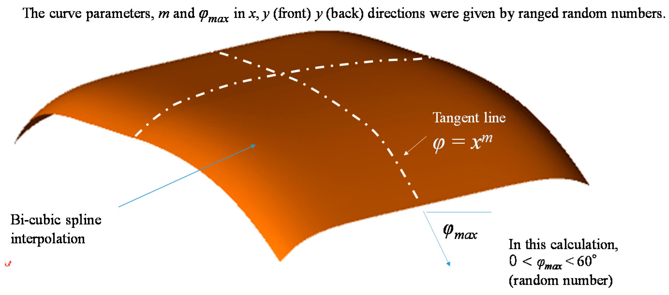
2.5.2. Examples of the Curve-Correction Calculations

A PV module with a curved surface is different from a flat plate module on power output. Specifically, the self-shielding effect of shielding a part of the incident from a shallow angle on its convex surface, the local cosine loss at each point of the solar cell is not constant, and due to the above factors, a mismatching loss further reduces the power output. That is, the output of the curved module has a different output value from the performance test with a conventional solar simulator designed for a flat plate, as we discussed in the previous section. Nonetheless, the exact test method of synthesizing the separately measured outputs by decomposing the curved surface into little surface elements (approximating each surface element to a very flat plate) is scarce in reality [25]. Therefore, a method of considering the power generation output on the 3D curved surface by multiplying the value measured by assuming the curved module as a 2D flat plate by the curve correction factor was studied. This curve correction factor is convenient because it can be uniquely determined for each curved surface given the incidence angle characteristics of the module and the incidence angle distribution of the solar cell if the mismatching loss is neglected.
The curve correction factor can be calculated by numerical, geometric calculation [35] or ray-tracing simulation [1]. For the geometrical calculation, it is important to add two conditions for avoiding complexity. First, the module does not absorb the light in the backside. Second, the curved surface is simple convex (no two or more peaks), namely the partial derivative functions of the profile function of the curved surface concerning x and y have no more than two points of the zero-crossing.
The curve correction factor f is defined as Equation (19).
P = A I f η
where P is the output of the module, A is a flattened area of the panel (not projected area), I is irradiance of the curved roof, f is the curve-correction factor, and η is the module efficiency measured by the flat condition by the conventional solar simulator. The curve correction factor f is a unique value depending on the 3D curve shape of the panel if the angular distribution of the solar irradiance is given. It is typically calculated by a numerical calculation (calculation algorithm should be open, transparent, and repeatable within some acceptable numerical errors, i.e., use of the Monte Carlo method). It should apply to the 3D CAD (computer-aided design) interface (most of the car roof 3D shapes were not simple polynomials but segmented smooth functions).
The curve correction factor f can be expressed as the product of two parameters (Equation (20)).
f = f 1 f 2
where, f1 is the coving factor, or in another way, geometrical curve correction factor corresponding to the ratio of the projected area by surface area, f2 is the irradiance ratio due to the local cosine loss and self-shading loss, in other words, optical curve correction factor. The parameter f1 may represent the overall shape of the curved surface.

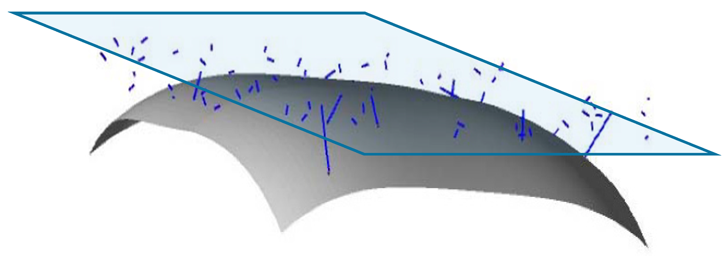
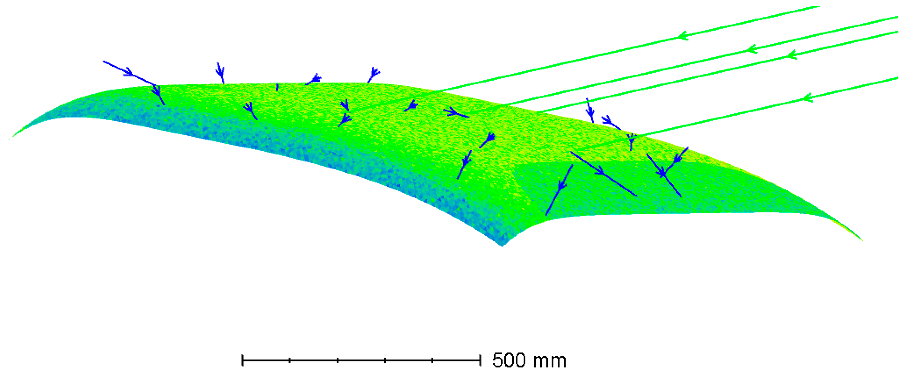
2.5.3. Curve-Correction Calculation Based on Ray-Tracing Simulation

The basic idea of the curve correction factor is the ratio of the absorbed flux and that of the light source with the area of the projected area of the curved PV panel that is placed just on the curved PV panel (Figure 7). The line segment around the light source (semi-transparent light-blue area) corresponds to the rays emitted from the light source. The short line segments correspond to the ray that does not reach to the curved surface. The longer line segments correspond to the one that hits the curved PV panel (curved opaque gray surface), namely the ray that is absorbed by the PV. Note that some rays just above the curved PV panel do not hit the curved module due to its curvature. To avoid the situation, the real light-source was placed on the surface of the virtual source plane (semi-transparent light-blue area) with a ten times larger area than the virtual light source. A detector is placed on the virtual light source and measures the total flux that passes the aperture zone (corresponding to the projected area) and compares the total flux absorbed by the curved PV surface (opaque gray surface). Note that the absorption at the backside surface is disabled in this calculation. The angular characteristics of the absorption are assumed as a Lambertian surface.
The curve correction factors of the various shape of the car roof are calculated and plotted in Figure 8; each corresponding marker in the plot was given by the random numbers. The curve shape of the car roof widely varies. Random numbers model each surface with an approximation of the bi-cubic spline function structured by the power function of the tangent lines (Figure 1). The curve shape profile is approximated as the segmented (symmetrical to left–right direction, but asymmetrical to front–back direction) power function constrained by the maximum slope at the edges. Specifically, it keeps symmetry in the X direction, but allows asymmetry in the Y direction, considering that the curve shape of the car roof may vary in the front and tail of the car body. The synthesis calculation is illustrated in Figure 9.
The curve correction factor decreases by the increase of curvature of the surface [20], corresponding to the ratio of the projected area by surface area (Figure 8). The geometrical factor f1 dominates it, but the optical curve correction also decreases by the increase of the curvature as well. However, the optical influence depends on the surface shape, and it is essential to calculate its factor to every curve surface.
The above approach can simulate the distribution of the solar irradiance of the curved car roof PV panel. To do this, it is necessary to specify the orientation of the panel, sun height, and ratio of the direct and scattered components. It is not appropriate to use the statistical distribution of the incident angle data because the distribution depends on the direction of the direct sunlight.
The distribution of the irradiance varies by both sun height and orientation angle. Unlike the BIPV, the orientation angle of the car roof PV varies by time. Such non-uniformity is observed by the measurement of the mini-module attached to various places on the car roof [33].
To avoid complexity, the validation by the measurement in this article does not consider the non-uniformity and the resultant mismatching loss in the module, but only considers the total flux absorbed by the module. The mismatching loss is handled separately by a Monte Carlo simulation, but it is not validated in this article. Although the mismatching loss due to non-uniformity may be expected, it will be significantly relaxed by the appropriate string design [24], and thus less significant than the reduction of the total flux.
The curve correction factor is also affected by the angular distribution of the solar irradiation. Roughly, the angular distribution of the sunlight in the horizontal surface moves to the higher incident angle when the sun height is low, thus higher latitude, lower average height of the shading objects, and seasonal fluctuation of the sunshine duration are high in winter, like the area of the south-east side of mountains in Asian monsoon regions.
The curve correction factors, f and f2, significantly vary by the site conditions, including latitude, climate pattern, and shading environment (urban zone or rural zone). This is because of the difference in the distribution of the incident angle onto the curved surface (Figure 10).

2.6. Partial and Dynamic Shading Model

The shading influence is complicated and varies by the position and the relative orientation (to the sun position) of the panel. In the case of the car roof PV, the position (orientation) of the panel cannot be predicted. One practical approach is to rely on the probability model, supposing that the distribution and height of the shading objects are randomly distributed by some statistical model and the orientation of the car is independent and random as well.
Most of the PV on the car roof is curved, which induces the non-uniform illumination caused by areal variation of the local cosine loss and self-shading loss. Such non-uniform illumination caused by the curved surface is equivalent to the partial shading given by the non-uniform photo-current output from each solar cell. A ray-tracing simulation can estimate such non-uniformity (Figure 11).
The above approach simulates the distribution of the solar irradiance of the curved car roof PV panel. To do this, it is necessary to specify the orientation of the panel, sun height, and ratio of the direct and scattered components. It is not appropriate to use the statistical distribution of the incident angle data because the distribution depends on the direction of the direct sunlight.
The distribution of the irradiance varies by both sun height and orientation angle. The orientation angle of the car roof PV varies by time. Such non-uniformity is observed by the measurement of the mini-module attached to various places on the car roof [23].
As was discussed in the previous sections, car roof PV is often partially shaded or receives equivalent non-uniform illumination caused by its basic curved shape. Both partial shading and non-uniform illumination can be simultaneously and quantitatively modeled, considering that both primarily effect variation of the short-circuit current of the cells.
For simplicity, cells in a module are categorized into three types.
  • In the sun
  • Full shade
  • Partial shade
Cells in the sun are supposed to be illuminated by all the sunlight, including direct sunlight; the shaded cells do not receive the direct component of the sunlight but instead receive diffused sunlight + reflected sunlight.
Random numbers give the number of the shaded cells (both full shaded and partially shaded) with some constraints. Random numbers also give the ratio of the shaded area of each partially-shaded cell. Random numbers give the position of the sun that affects the angle of the sunbeam and the orientation of the car roof as well. Finally, the I–V curve of each cell is calculated by three randomly distributed parameters (normal distribution). The property of the probability variables used for the Monte Carlo simulation is summarized in Table 1. The irradiance and climate conditions corresponding to the above parameters are found in the METPV-11 [45] and METPV-ASIA [46] databases. Given these probability parameters, I–V curves of entire cells in the array affect different illumination conditions, and variations of characteristics are calculated, and the maximum power point is calculated for taking the simulated power output affected by the partial shading.
It is important to note that the probability modeling of the partial shading, corresponding to the fourth through sixth rows of Table 2, is the key to the simulation. To minimize the evil influence of the partial shading, the PV and car manufacturers try to place the series strings as close as possible to the shape of the partial shading or non-uniform illumination pattern caused by the curvature of the car body. In a way, the distribution of the shaded cells are not uniformly distributed but leaves some distribution pattern. To mimic this situation, the random model is made by three steps (see fourth to sixth rows of Table 1). Specifically, the number of the shaded cells in each string is allocated using Equation (21), and the short-circuit current from each cell impacted by shading is given in Equation (2). Note both Equations (1) and (2) contain Boolean algebra. It is also important to note that the vector and matrix data that are generated by the above calculations and contain the information of the shaded ratio of each cell in the module are only used as the circuit calculation of the module by series-parallel connection with bypass diodes. Therefore, in the downstream calculation step, the position of the shaded cell is not referenced, but they may be redistributed in the series connection by order of the shaded ratio.
Applsci 10 00872 i001
I r i , j = S T I + ( ( j < S c n i ) + i f ( ( S c n i j < S n p i + S c n i ) S n p i > 0 ,   r u n i f ( S n p i ,   0 ,   1 ) j S c n i ,   0 ) ) · D T I T I S
where SF(n, Nstrings) is a function that generates a vector containing the number of shaded cells in each string. n is a scalar parameter of the number of cells in a string. Nstrings is a scalar parameter of the number of strings in a module. floor(z) is a function that returns the greatest integer ≤ z. rnd(x) is a function that returns a uniformly distributed random number between 0 and x. if(cond, x, y) is a function that returns x if cond is true (nonzero), y otherwise. stack(A, B, C, ...) is a function that returns an array formed by placing A, B, C, ... top to bottom. submatrix(A, ir, jr, ic, jc) is a function that returns the matrix consisting of rows ir through jr and columns ic through jc of array A. Ir in Equation (22) is an array that contains solar irradiance of each cell in the module affected by partial shadings. STI is a scalar parameter of the diffused sunlight onto the module plane. Scn is a vector that contains a number of the unshaded cells in each string in the module. Snp is a vector that contains a number of partially shaded cells in strings. runif(m, a, b) is a function that returns a vector of m random numbers with uniform distribution, and m is a scalar of real values, amb. To allow integration and other operations over this argument, values outside of the stated range are allowed, but they produce a 0 result. a and b are real numbers, a < b. DTI is a scalar parameter of the direct sunlight onto the module plane. TIS is a scalar parameter of the total sunlight onto the module plane.

3. Results

In this article, we evaluate the annual irradiance incident on the car using five pyranometers located in five orthogonal directions. We also present the seasonal variation of the angular distribution of the leading solar beam and the annually angular distribution model on a car roof.

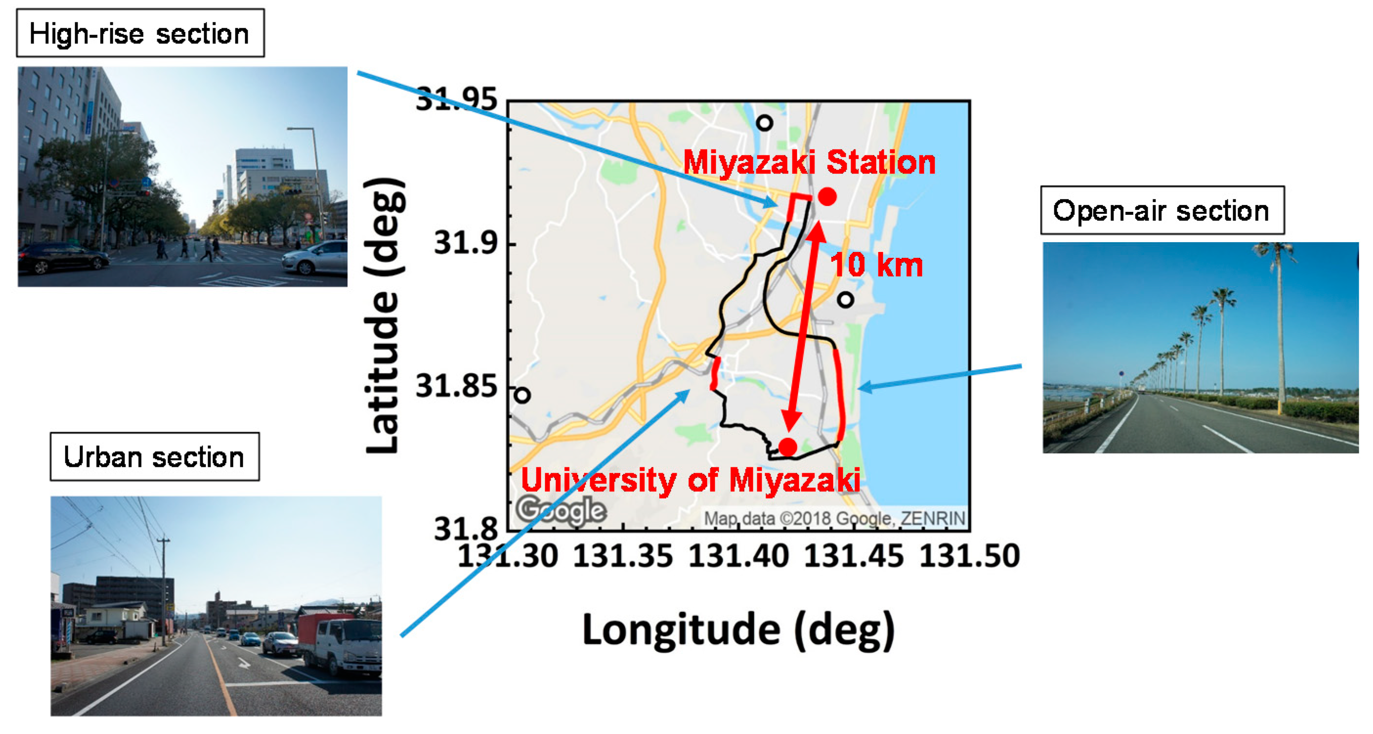
3.1. 3D Measurement by Multiple Pyranometer Array

The measurement system consists of five pyranometers mounted on the car roof, along with a GPS; thus, it could be moved on the road. The pyranometer axes Qx+, Qx−, Qy+, Qy−, and Qz are defined, as shown in Figure 12. One pyranometer is placed horizontally on the car roof (Qz), and four pyranometers are placed vertically facing each side of the car (Qx+, Qx−, Qy+, Qy−). The global irradiance onto the car roof (Iz) is measured using a pyranometer Qz. The global irradiance onto the side of the car (Ix+, Ix−, Iy+, Iy−) is measured using pyranometers Qx+, Qx−, Qy+, Qy−. The direction of the moving car is equal to that of Qy+. An ambient temperature meter (Pt 100 temperature sensor) is also placed on the car roof. The GPS is incorporated into the data logger, and data are recorded in 1 s intervals. The total number of hours of sun radiation (more than 10 W/m2 in Iz) received over the year was 3374 h, while the number of hours the car was running was approximately 6% of this.
To acquire a dataset for comparison, a conventional static irradiance measurement system with a pyrheliometer, a tracking pyranometer mounted onto a sun tracker, a horizontal pyranometer, and two vertical pyranometers facing eastward and westward was installed at the University of Miyazaki, Japan (31°49′ N, 131°24′ E). The elevation angle and azimuth angle of the sun position are calculated based on the conventional method, including the day angle, declination angle, time equation, hour angle, latitude, and longitude.

3.2. Measurement Example of the Solar Irradiance on the Car Roof and Car Side

The city of Miyazaki, Japan, is one of the capitals of local government in Japan (Miyazaki prefecture) with a population of approximately 200,000. Thus, this area contains an urban zone, a residential zone, and a rural zone. In a way, it may be a representative zone in the solar environment (shading frequency and shading height). We did not constrain the driving course of the one-year monitoring of the solar irradiance on the car, but the most frequent driving course of this car is shown in Figure 13 since it was used for commuting between the University of Miyazaki and the driver’s residence.
The typical monitored result in the route in Figure 13 is shown in Figure 14 (clear sky day) with comparison to the global horizontal irradiance (GHI) of fixed pyranometers (mounted on a roof of one of the buildings of the University of Miyazaki).
In the region of the open-air section, the solar irradiance on the car roof is almost identical to the GHI by the fixed pyranometers. However, that of other areas had frequent dips in the irradiance on the car. The timestamp and position data taken by GPS confirmed that these are because of the shading effects by buildings and mountains. The car roof irradiance often exceeded GHI. It is also confirmed because of the reflectance of the buildings.

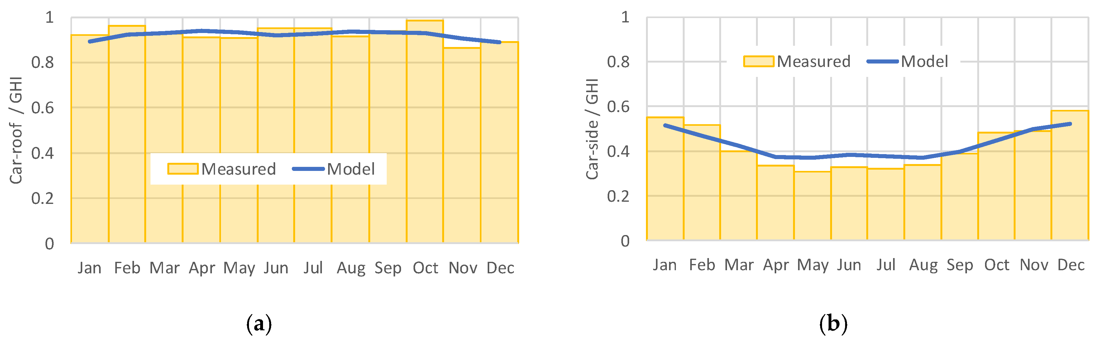
3.3. Validation of the Solar Irradiation Model around the Car (Intensity)

The above model was compared with the one-year observation result of the solar irradiance to the vehicle, including seasonal (monthly) fluctuation. After fitting to the measurement irradiance dataset, the fitted average shading height is 18.7° in the direction along the road (local axis) and 12.3° in the direction orthogonal to the road (local axis), and 15.5° as the average. The averaged shading height after data fit was 15.5°, and it is very close from the value of rough physical measurement (15° on average). The average reflectance from the road is also fit to the measured data and obtained as 0.088, also a reasonable value for aged asphalt (typical value is 0.07). The comparison to the measured irradiance and modeled irradiance are compared in Table 2.
The validation is also done by a one-month integration (seasonal fluctuation). The model met the modeled values in every month (Figure 15). The trend of the residual errors could be explained by the difference in climate from the regular year (for example, cloudy in summer).
The same comparison is made on a daily base (Figure 16). Since every day’s climate is not always identical to the one in the solar database, there are significant errors in the time-series trend. However, the range of the distribution in the modeled irradiance is almost the same as the measured irradiance.

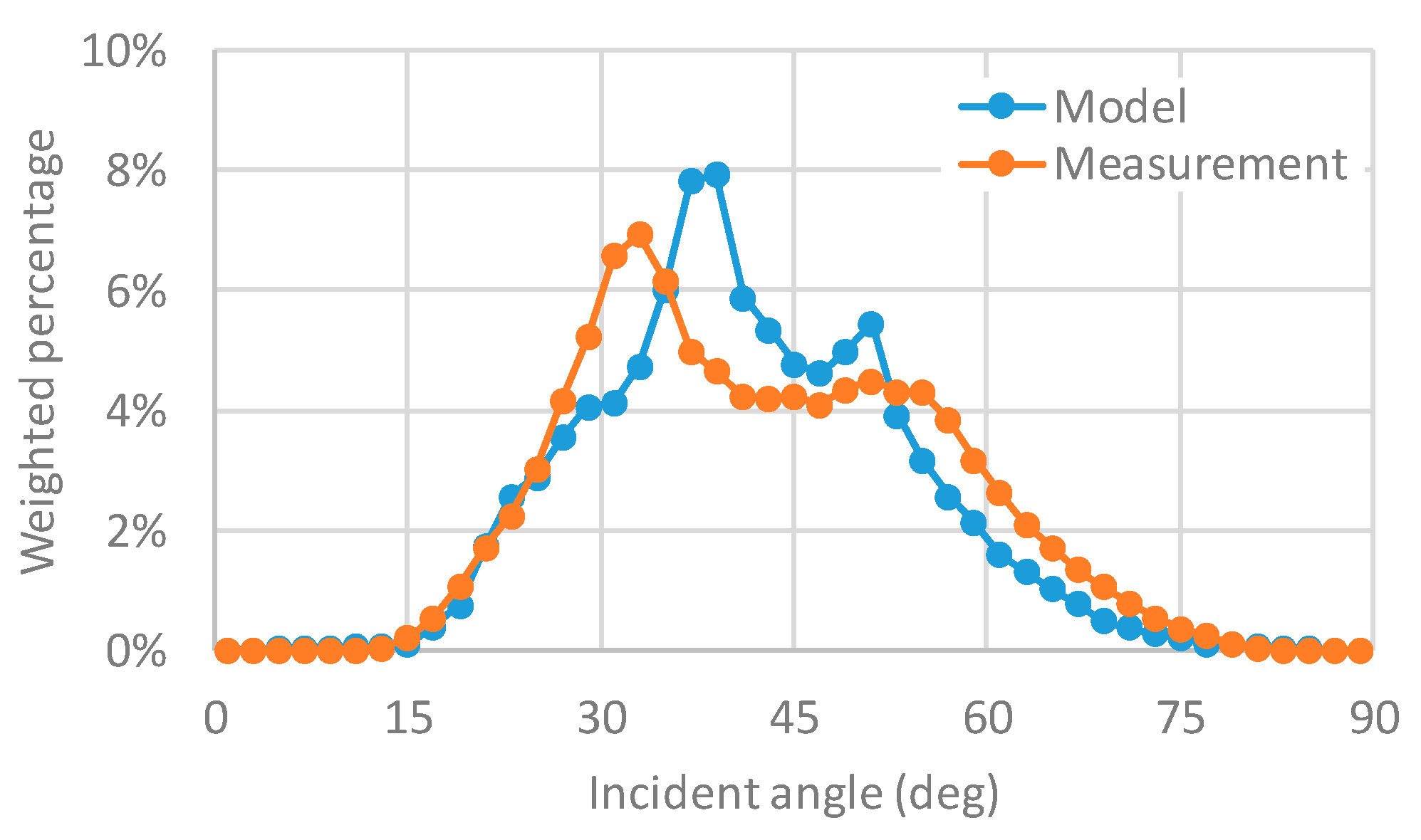
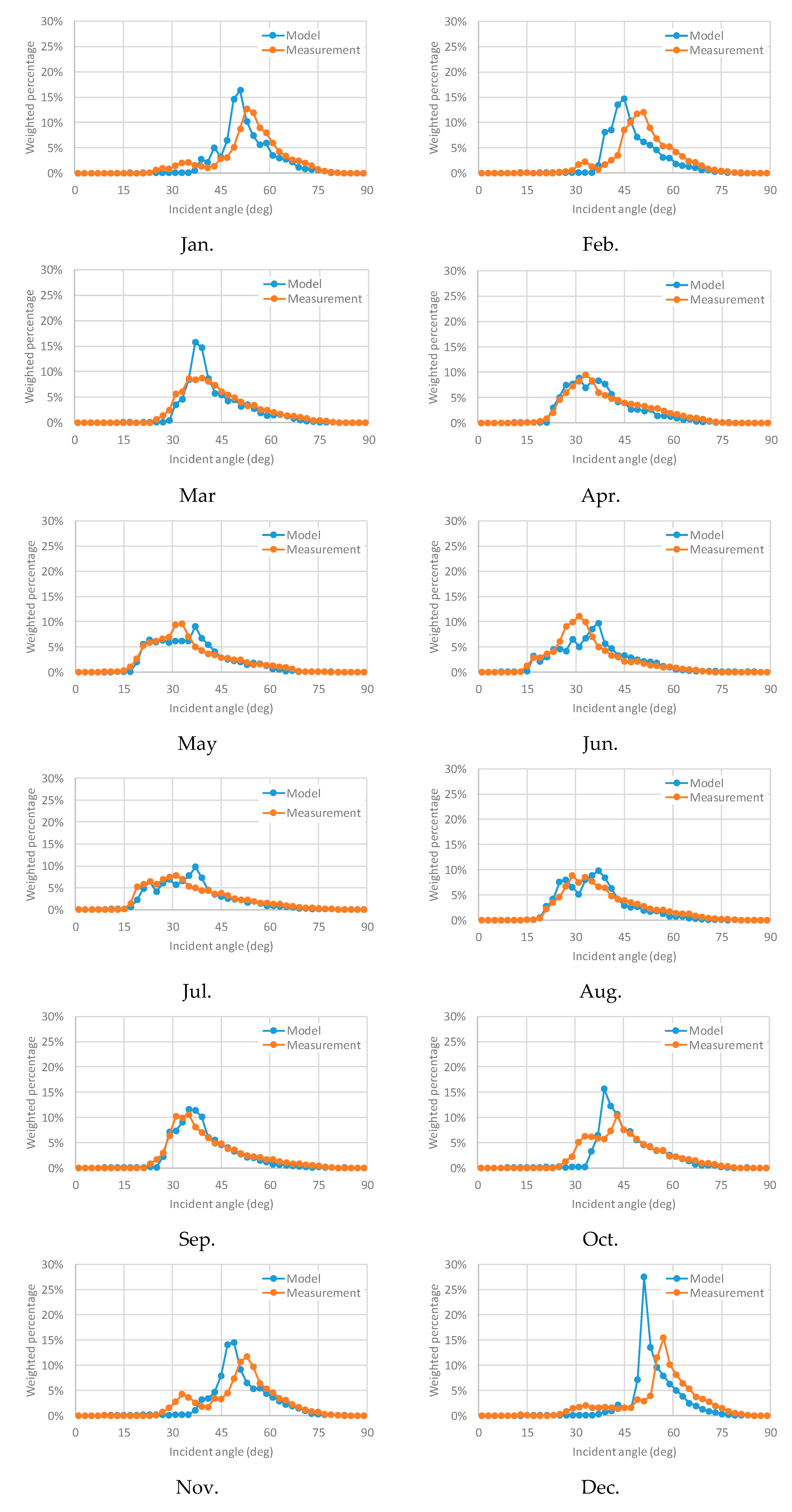
3.4. Validation of the Solar Irradiation Model around the Car (Angle)

After validation of the irradiance model affected by the surrounding shading objects, the histogram of the car irradiance is counted using the one-year irradiation model. The results of annually integrated angular distribution are shown in Figure 17. For examining the seasonal trend, the weighted histograms of the angular distribution of the leading solar beam in each month are plotted in Figure 18. The residual error of the model is observed in more than 30° of incident angle or winter season (corresponding low sun height and high incident angle). It is possible because the model of the shading height distribution is too simplified. However, the overall trend meets the measured one, and the angular model can be used for a rough estimation of the solar irradiance environment around the car body.

4. Discussion

4.1. Simplified Rating Method of VIPV Considering 3D Solar Irradiance

The standard rating measurement for PV is done by a single measurement in the normal illumination. However, that of VIPV is not sufficient because it uses three-dimensional solar irradiance by a curved module and three-dimensional installation (frequently, the PV module on the car side is added).
The ratio of solar resource measurement is useful for a quick rating of the VIPV system on the car by three-dimensional measurement. Possible steps are as follows:
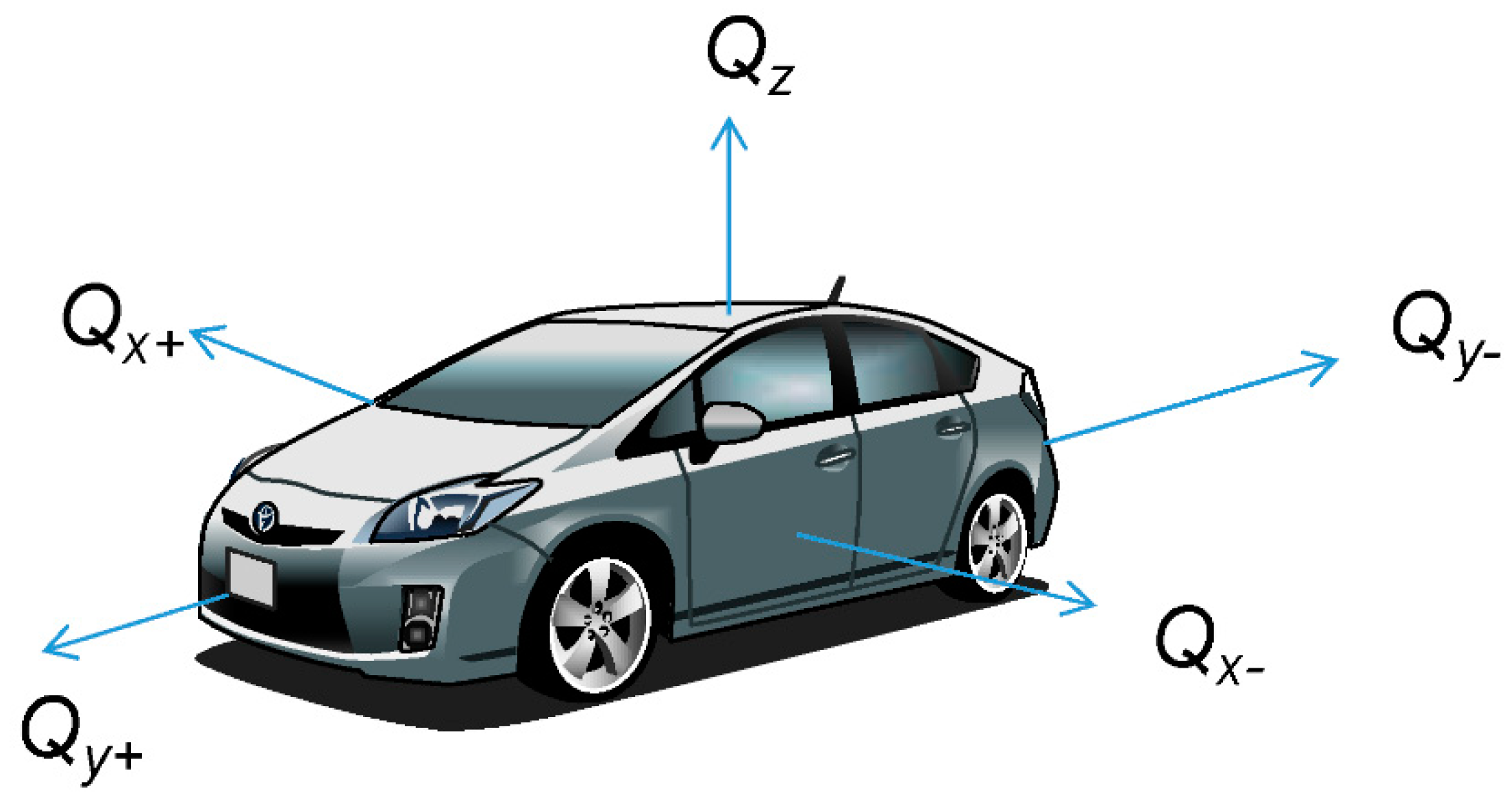
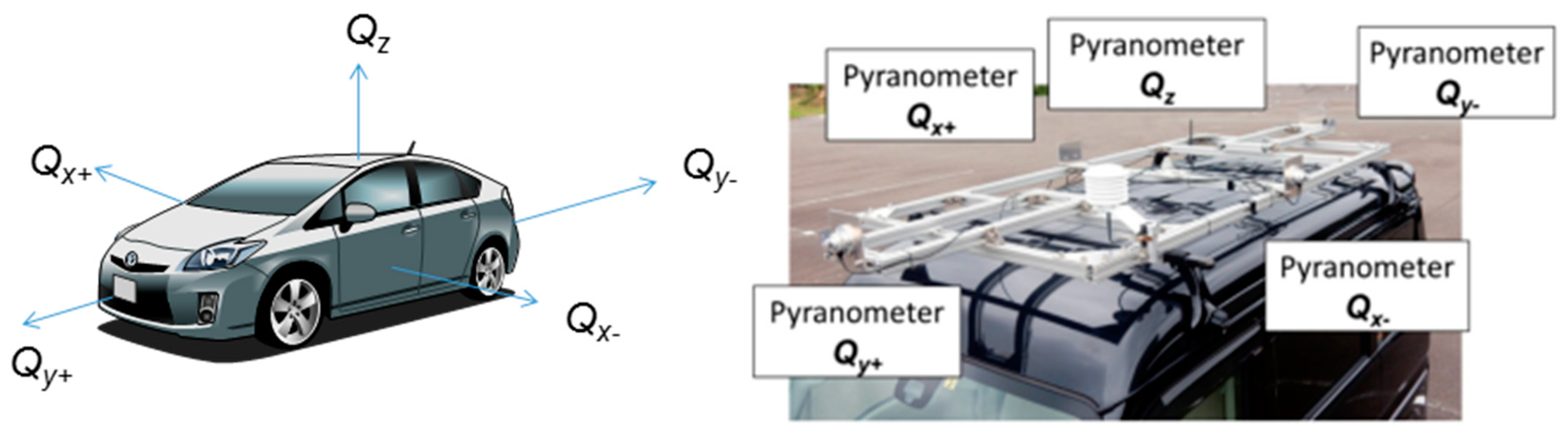
  • Measure the PV performance in five directions (see Figure 2).
  • The rating of the total performance in the specific area can be weighted by the normalized solar resources using Equation (23) and the values in Table 2, namely,
    P = a P z + b ( P x + + P x ) + c ( P y + + P y )
    where P is the rated power output. Pz is the measured power output by the illumination on the car roof. Px+, Px−, Py+, and Py1 are the measured power outputs by the illumination on the car sides in the direction defined in Figure 1. a, b, and c are weighting coefficients given by Table 2. Note that the coefficients a, b, and c in our measurement in Miyazaki, Japan are 0.925, 0.395, and 0.435, respectively. Equation (21) gives a total energy output of the entire PV system on the vehicle considering 3D solar irradiance around the vehicle comparable to GHI.

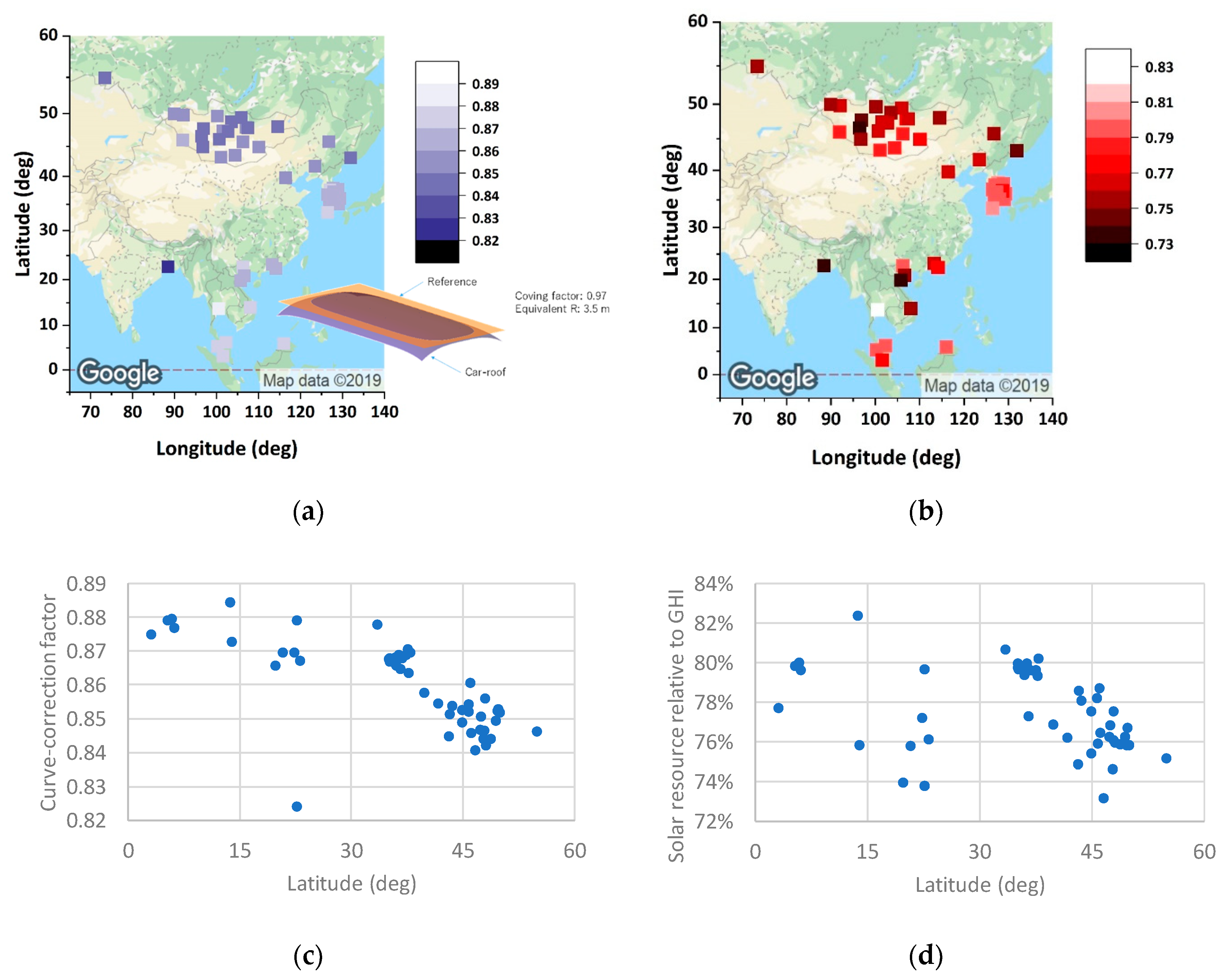
4.2. Estimation of the Practical Solar Resource to VIPV in Other Regions

Assuming that the density and height distribution of the shading objects are the same to that of Miyazaki, Japan, namely the average shading height is about 15.5°, it may be possible to anticipate the energy yield of the VIPV in various area in the world; this is useful to anticipate the merits of the introduction of solar-driven vehicles.
Figure 19 indicates the map of the practical solar resource on the car roof normalized to the GHI, affected by climate conditions. They are calculated using a model in Section 2.2 and Section 2.5, using METPV-ASIA solar irradiance database. Due to the shading impact and curved surface, the practical solar resource for the car roof is less than the typical installation. The rough value may be 3/4 of the GHI.
Generally speaking, both the shading impact and curve impact increases with the decrease of the sun height, namely, increasing the latitude. However, both curve-correction factor and effective solar resource to the car roof normalize to GHI (including the loss by the curved surface), do not show a strong correlation to latitude (thus sun height), and unlike other typical solar resource parameters, is affected by local meteorological conditions. Also, note that both the curve-correction factor and the effective solar resource relative to GHI are strongly affected by the distribution (both special and height) of shading objects.

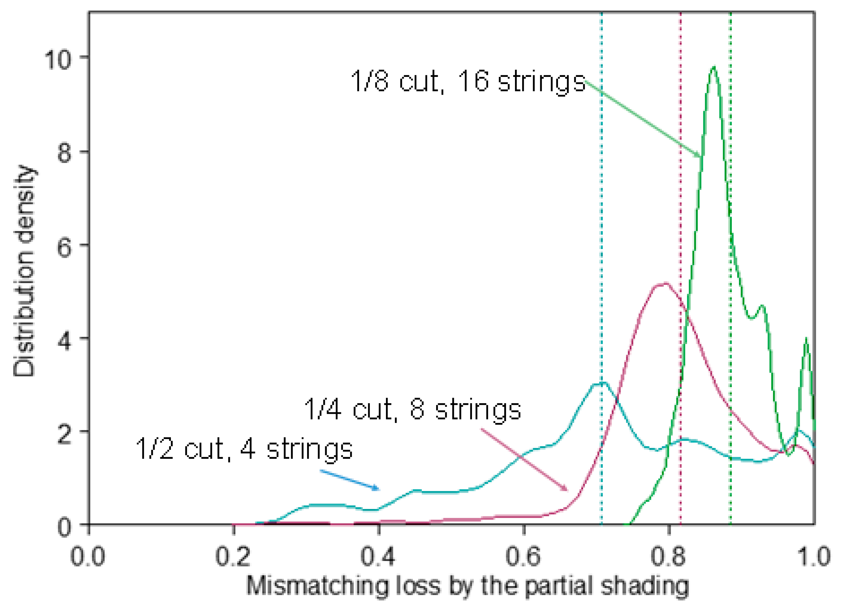
4.3. Partial Shading Issue

Since calculated power and related loss are affected by probability variables, the calculated result is not a single number but shows a distribution. Figure 20 shows an example of the distribution of the normalized efficiency of several array designs of the car roof PV, affected by the mismatching loss result from partial shading. The ratio of the power output of the partially shaded module is less than the ratio of the area in the sun. The reduction ratio corresponds to the mismatching loss. The loss factor is a function of the number of strings, curvature of the car roof, and latitude.

4.4. Limitation of the Model

First, the model discussed in this article relies on the random number and assumes that every parameter affecting the solar resource on the car roof and car side is distributed by a simple rule, for example, ranged uniform distribution. It may be meaningful to the averaged or integrated energy yield but cannot be applied to the power prediction in specific driving points and directions, specific climate as well as specific surrounding conditions. The given distributions may not be equal to the real situation that varies every position and every time. In this sense, it is to be applied to annual or other long-term integration like annual energy yield.
Distribution of the shading objects (both spatial distribution and height distribution) is essential to the model. Our model is based on a linear trend (Figure 2) but is too simplified to the shading in the high-rise section in Figure 13, where the trend of Figure 2 may become trapezoid or other complicated shapes. Namely, the energy yield in the urban area may give an optimistically-biased value.
For the moment, the impact by the partial shading has not been considered yet. We only estimated the impact of using a Monte Carlo simulation. Depending on the string configuration or the power-conditioner connected to the car-mounted module, the output power may drop by the mismatching loss that was not anticipated to the model.

4.5. Feasibility of the VIPV Based on Our Measurement and Modeling

Compared with the past reports by Toyota Motors [2] and New Energy and Industrial Technology Development Organization (NEDO) [3] which did not consider the shading effect by surrounding objects and loss by the curved surface, our research gives a more realistic solar resource on the car roof and car side. These two reports gave an overestimation of the energy yield expectation. The rough number suggested by this research is around 3/4 using highly curved PV modules on the car roof and shading effects (taken by the capital of the local government in Japan).
As it is measured and modeled in this study, the energy yield of VIPV is undoubtedly less than that of the PV power plant that is constructed maximizing the energy yield by a given amount of the solar panels. However, considering that the related soft-cost and other balance of system costs (construction, structure, connecting to the grid, distribution, and the cost of the constructing and operation of the EV charging station) that are to be eventually shared by car owners or car manufacturers, VIPV will be attractive option both in cost and user-friendliness.

4.6. Future Works

For improvement of the energy yield prediction of VIPV, the following works are to be done.
  • Improvement of the shading model. The current model is useful but too simplified, especially in the urban area. Note that more than 45° of the average shading height is not allowed, because the maximum height becomes more than 90°. Even in the area of Miyazaki, the average height of 15.5° means that the maximum height should be 31°. However, there are many buildings of more than 31°. Possibly, we need to develop a curved trend, namely the two parameters model.
  • Modeling of partial shading validated to the measured data. To do this, we need to start monitoring the partial shading on the car roof and car body.
  • Validation of energy yield using the real curved PV module.
  • Validation of the shading model by several areas with different shading height and shading density.
  • Development of the spectrum model for predicting energy yield by multi-junction solar cells on the car roof and car body.

5. Conclusions

As a result of increasing concerns of greenhouse gas emissions in the transportation sectors, the fuel and engine of the car are required to consider the total emission of CO2 on a well-to-wheel basis. The typical approach is an electric vehicle (EV) [47] charged by the electricity generated by renewable energy like solar power [48]. The primary energy should be renewable energy; otherwise, a significant reduction of the greenhouse gas emission will not be expected [49]. However, this approach relies on the infrastructure of the distribution of clean electricity (PV power station installation, grid construction and connection, distribution of the clean electricity, and installation and operation of the EV charging station). It is much more convenient that the car collects solar energy and runs by it (or at least extending the range of mileage supported by its PV modules to reduce the frequency of charging).
Solar-powered vehicles are now seriously discussed, and we have several feasibility reports [2,3]. In principle, it is feasible by the improvement of both PV and car technologies to run a majority of electric vehicles on solar energy. However, as it is often the case of the early feasibility study, it is not supported by the real solar resources of the car running in the real environment. The motivation for our study is to know the real and active solar energy for the car through both modeling and measurement.
For modeling, we developed a simple shading model using uniformly distributed (density and height) shading objects and random driving orientation using a simple combination of the collimated direct sunlight, uniform diffused sunlight, and reflection by road and shading objects. For the validation of the model, we used an array of pyranometers mounted on the car in five axes and monitored the solar resource around the car for one year. The model was validated in x, y, and z-directions local to the car as well as the angular distribution of the main beam of the solar irradiance on the car roof.
Additionally, we developed the curved surface of the car roof and car body using the correction method. Commonly the car roof and car body are curved, and car manufacturers want PV panels that are also curved to fit the car body. The measurement (indoor testing) and performance (outdoor operation) in the standard PV panel was established by the fact that the PV panel always has a flat surface. We had to construct both the testing method and operation model from the beginning considering the three-dimensional density of the photon energy absorbance. Our solution is to introduce a curve-correction factor that keeps compatibility with the current testing equipment and standards. The curve-correction factor can be calculated by the ray-tracing calculation, once both the curve profile (possibly by CAD file) and angular distribution of the solar irradiance (also given by those mentioned above by the new solar resource model on the car body).
Another crucial factor that affects energy yield from the VIPV is the mismatching loss either by the partial shading or non-uniform distribution by the curved surface. Currently, we developed a Monte Carlo simulation assuming that random numbers give the non-uniformity and ratio of the partial shading.
Here is a summary of the conclusion in technical issues:
  • A simple shading model to VIPV was developed and validated by one-year monitoring on the solar irradiation on the car roof and car body in five axes.
  • The curve-correction model of the curved surface of VIPV was developed.
  • A mismatching model using Monte Carlo simulation was developed to analyze the partial shading of VIPV.

Author Contributions

Conceptualization, K.A.; methodology, Y.O.; software, K.A.; validation, Y.O.; investigation, Y.O.; data curation, Y.O.; writing—original draft preparation, K.A.; writing—review and editing, Y.O.; visualization, K.A., and Y.O.; supervision, Y.O.; project administration, M.Y.; funding acquisition, M.Y. All authors have read and agreed to the published version of the manuscript.

Funding

Part of this research was funded by the New Energy and Industrial Technology Development Organization (NEDO) under the Ministry of Economy, Trade, and Industry (METI), Japan.

Acknowledgments

The modeling of VIPV was first discussed in the international web meetings (76 scientists and engineers are registered) for the standardization of the car roof PV, starting discussions in December 2017. Part of this research was funded by NEDO, Japan. The standardization activities were supported by JEMA, Japan.

Conflicts of Interest

The authors declare no conflicts of interest.

References

  1. Araki, K.; Ji, L.; Kelly, G.; Yamaguchi, M. To Do List for Research and Development and International Standardization to Achieve the Goal of Running a Majority of Electric Vehicles on Solar Energy. Coatings 2018, 8, 251. [Google Scholar] [CrossRef] [Green Version]
  2. Masuda, T.; Araki, K.; Okumura, K.; Urabe, S.; Kudo, Y.; Kimura, K.; Nakado, T.; Sato, A.; Yamaguchi, M. Static concentrator photovoltaics for automotive applications. Sol. Energy 2017, 146, 523–531. [Google Scholar] [CrossRef]
  3. NEDO. Interim Report of the Exploratory Committee on the Automobile Using Photovoltaic System. Available online: http://www.nedo.go.jp/news/press/AA5_100909.html (accessed on 9 May 2018).
  4. Masuda, T.; Araki, K.; Okumura, K.; Urabe, S.; Kudo, Y.; Kimura, K.; Nakado, T.; Sato, A.; Yamaguchi, M. Next environment-friendly cars: Application of solar power as automobile energy source. In Proceedings of the IEEE 43rd Photovoltaic Specialists Conference (PVSC), Portland, OR, USA, 5–10 June 2016; pp. 580–584. [Google Scholar]
  5. Araki, K.; Sato, D.; Masuda, T.; Lee, K.H.; Yamada, N.; Yamaguchi, M. Why and how does car roof PV create 50 GW/year of new installations? Also, why is a static CPV suitable to this application? In AIP Conference Proceedings; AIP Publishing: Melville, NY, USA, 2019; Volume 2149, p. 050003. [Google Scholar]
  6. Stutzmann, M. Role of mechanical stress in the light-induced degradation of hydrogenated amorphous silicon. Appl. Phys. Lett. 1985, 47, 21–23. [Google Scholar] [CrossRef]
  7. Moeini, I.; Ahmadpour, M.; Mosavi, A.; Alharbi, N.; Gorji, N.E. Modeling the time-dependent characteristics of perovskite solar cells. Sol. Energy 2018, 170, 969–973. [Google Scholar] [CrossRef]
  8. Lindroos, J.; Savin, H. Review of light-induced degradation in crystalline silicon solar cells. Sol. Energy Mater. Sol. Cells 2016, 147, 115–126. [Google Scholar] [CrossRef]
  9. Meyer, E.L.; Van Dyk, E.E. Assessing the reliability and degradation of photovoltaic module performance parameters. IEEE Trans. Reliab. 2004, 53, 83–92. [Google Scholar] [CrossRef]
  10. Letendre, S.; Perez, R.; Herig, C. Vehicle integrated PV: A clean and secure fuel for hybrid electric vehicles. In Proceedings of the Solar Conference; American Solar Energy Society: Boulder, CO, USA; American Institute of Architects: Washington, DC, USA, 2003; pp. 201–206. [Google Scholar]
  11. De Pinto, S.; Lu, Q.; Camocardi, P.; Chatzikomis, C.; Sorniotti, A.; Ragonese, D.; Iuzzolino, G.; Perlo, P.; Lekakou, C. Electric vehicle driving range extension using photovoltaic panels. In Proceedings of the IEEE Vehicle Power and Propulsion Conference (VPPC), Hangzhou, China, 17–20 October 2016; IEEE: Piscataway, NJ, USA, 2016; pp. 1–6. [Google Scholar]
  12. Kim, J.; Wang, Y.; Pedram, M.; Chang, N. Fast photovoltaic array reconfiguration for partial solar powered vehicles. In Proceedings of the International Symposium on Low Power Electronics and Design, La Jolla, CA, USA, 11–13 August 2014; pp. 357–362. [Google Scholar]
  13. Alhammad, Y.A.; Al-Azzawi, W.F. Exploitation the waste energy in hybrid cars to improve the efficiency of solar cell panel as an auxiliary power supply. In Proceedings of the 10th International Symposium on Mechatronics and its Applications (ISMA), Sharjah, UAE, 8–10 December 2015; IEEE: Piscataway, NJ, USA, 2016; pp. 1–6. [Google Scholar]
  14. Fujinaka, M. The practically usable electric vehicle charged by photovoltaic cells. In Proceedings of the 24th Intersociety Energy Conversion Engineering Conference, Washington, DC, USA, 6–11 August 1989; IEEE: Piscataway, NJ, USA, 2002; pp. 2473–2478. [Google Scholar]
  15. Ezzat, M.F.; Dincer, I. Development, analysis and assessment of a fuel cell and solar photovoltaic system powered vehicle. Energy Convers. Manag. 2016, 129, 284–292. [Google Scholar] [CrossRef]
  16. Araki, K.; Ota, Y.; Nishioka, K.; Tobita, H.; Ji, L.; Kelly, G.; Yamaguchi, M. Toward the Standardization of the Car-roof PV—The challenge to the 3D Sunshine Modeling and Rating of the 3D Continuously Curved PV Panel. In Proceedings of the IEEE 7th World Conference on Photovoltaic Energy Conversion (WCPEC) (A Joint Conference of 45th IEEE PVSC, 28th PVSEC & 34th EU PVSEC), Waikoloa Village, HI, USA, 10–15 June 2018; pp. 368–373. [Google Scholar] [CrossRef]
  17. Araki, K.; Algora, C.; Siefer, G.; Nishioka, K.; Leutz, R.; Carter, S.; Wang, S.; Askins, S.; Ji, L.; Kelly, G. Standardization of the CPV and car roof PV technology in 2018—Where are we going to go? AIP Conf. Proc. 2018, 2012, 070001. [Google Scholar]
  18. Araki, K.; Algora, C.; Siefer, G.; NIshioka, K.; Muller, M.; Leutz, R.; Carter, S.; Wang, S.; Askins, S.; Ji, L.; et al. Toward Standardization of Solar trackers, concentrator PV, and car-ROOF pv. Grand Renew. Energy Proc. Jpn. Counc. Renew. Energy 2018, 2018, 37. [Google Scholar]
  19. Araki, K.; Algora, C.; Siefer, G.; Nishioka, K.; Leutz, R.; Carter, S.; Wang, S.; Askins, S.; Ji, L.; Kelly, G. Standardization of the CPV technology in 2019—The path to new CPV technologies. In AIP Conference Proceedings; AIP Publishing: Melville, NY, USA, 2019; Volume 2149, p. 090001. [Google Scholar]
  20. Ota, Y.; Masuda, T.; Araki, K.; Yamaguchi, M. Curve-Correction Factor for Characterization of the Output of a Three-Dimensional Curved Photovoltaic Module on a Car Roof. Coatings 2018, 8, 432. [Google Scholar] [CrossRef] [Green Version]
  21. Schuss, C.; Kotikumpu, T.; Eichberger, B.; Rahkonen, T. Impact of dynamic environmental conditions on the output behaviour of photovoltaics. In Proceedings of the 20th IMEKO TC-4 International Symposium, Benevento, Italy, 15–17 September 2014; pp. 993–998. [Google Scholar]
  22. Schuss, C.; Gall, H.; Eberhart, K.; Illko, H.; Eichberger, B. Alignment and interconnection of photovoltaics on electric and hybrid electric vehicles. In Proceedings of the IEEE International Instrumentation and Measurement Technology Conference (I2MTC) Proceedings, Montevideo, Uruguay, 12–15 May 2014; pp. 153–158. [Google Scholar]
  23. Schuss, C.; Eichberger, B.; Rahkonen, T. Impact of sampling interval on the accuracy of estimating the amount of solar energy. In Proceedings of the IEEE International Instrumentation and Measurement Technology Conference Proceedings, Taipei, Taiwan, 23–26 May 2016; pp. 1–6. [Google Scholar]
  24. Araki, K.; Lee, K.-H.; Masuda, T.; Hayakawa, Y.; Yamada, N.; Ota, Y.; Yamaguchi, M. Rough and Straightforward Estimation of the Mismatching Loss by Partial Shading of the PV Modules Installed on an Urban Area or Car-Roof. In Proceedings of the 46th IEEE PVSC, Chicago, IL, USA, 16–21 June 2019. [Google Scholar]
  25. Tayagaki, T.; Araki, K.; Yamaguchi, M.; Sugaya, T. Impact of Nonplanar Panels on Photovoltaic Power Generation in the Case of Vehicles. IEEE J. Photovolt. 2019, 9, 1721–1726. [Google Scholar] [CrossRef]
  26. Araki, K.; Ota, Y.; Lee, K.-H.Y.; Yamada, N.; Yamaguchi, M. Curve Correction of the Energy Yield by Flexible Photovoltaics for VIPV and BIPV Applications Using a Simple Correction Factor. In Proceedings of the 46th IEEE PVSC, Chicago, IL, USA, 16–21 June 2019. [Google Scholar]
  27. Ota, Y.; Masuda, T.; Araki, K.; Yamaguchi, M. A mobile multipyranometer array for the assessment of solar irradiance incident on a photovoltaic-powered vehicle. Sol. Energy 2019, 184, 84–90. [Google Scholar] [CrossRef]
  28. Araki, K.; Ota, Y.; Ikeda, K.; Lee, K.H.; Nishioka, K.; Yamaguchi, M. Possibility of static low concentrator PV optimized for vehicle installation. AIP Conf. Proc. 2016, 1766, 020001. [Google Scholar]
  29. Ota, Y.; Nishioka, K.; Araki, K.; Ikeda, K.; Lee, K.H.; Yamaguchi, M. Optimization of static concentrator photovoltaics with aspherical lens for automobile. In Proceedings of the IEEE 43rd Photovoltaic Specialists Conference (PVSC), Portland, OR, USA, 5–10 June 2016; pp. 570–573. [Google Scholar]
  30. Araki, K.; Lee, K.H.; Yamaguchi, M. The possibility of the static LCPV to mechanical-stack III-V//Si module. Aip Conf. Proc. 2018, 2012, 090002. [Google Scholar]
  31. Sato, D.; Lee, K.H.; Araki, K.; Masuda, T.; Yamaguchi, M.; Yamada, N. Design and Evaluation of Low-concentration Static III-V/Si Partial CPV Module for Car-rooftop Application. In Proceedings of the IEEE 7th World Conference on Photovoltaic Energy Conversion (WCPEC) (A Joint Conference of 45th IEEE PVSC, 28th PVSEC & 34th EU PVSEC), Waikoloa Village, HI, USA, 10–15 June 2018; pp. 954–957. [Google Scholar]
  32. Sato, D.; Lee, K.H.; Araki, K.; Masuda, T.; Yamaguchi, M.; Yamada, N. Design of low-concentration static III-V/Si partial CPV module with 27.3% annual efficiency for car-roof application. Prog. Photovolt. Res. Appl. 2019, 27, 501–510. [Google Scholar] [CrossRef]
  33. Ekins-Daukes, N.J.; Betts, T.R.; Kemmoku, Y.; Araki, K.; Lee, H.S.; Gottschalg, R.; Yamaguchi, M. Syracuse-a multi-junction concentrator system computer model. In Proceedings of the Conference Record of the Thirty-first IEEE Photovoltaic Specialists Conference, Lake Buena Vista, FL, USA, 3–7 January 2005; IEEE: Piscataway, NJ, USA, 2005; pp. 651–654. [Google Scholar]
  34. Tawa, H.; Saiki, H.; Ota, Y.; Araki, K.; Takamoto, T.; Nishioka, K. Accurate output forecasting method for various photovoltaic modules considering incident angle and spectral change owing to atmospheric parameters and cloud conditions. Appl. Sci. 2020, in press. [Google Scholar] [CrossRef] [Green Version]
  35. Araki, K.; Ota, Y.; Lee, K.H.; Nishioka, K.; Yamaguchi, M. Optimization of the Partially Radiative-coupling Multi-junction Solar Cells Considering Fluctuation of Atmospheric Conditions. In Proceedings of the IEEE 7th World Conference on Photovoltaic Energy Conversion (WCPEC) (A Joint Conference of 45th IEEE PVSC, 28th PVSEC & 34th EU PVSEC), Waikoloa Village, HI, USA, 10–15 June 2018; pp. 1661–1666. [Google Scholar]
  36. Araki, K.; Ota, Y.; Saiki, H.; Tawa, H.; Nishioka, K.; Yamaguchi, M. Super-Multi-Junction Solar Cells—Device Configuration with the Potential for More Than 50% Annual Energy Conversion Efficiency (Non-Concentration). Appl. Sci. 2019, 9, 4598. [Google Scholar] [CrossRef] [Green Version]
  37. Saiki, H.; Sakai, T.; Araki, K.; Ota, Y.; Lee, K.H.; Yamaguchi, M.; Nishioka, K. Verification of uncertainty in CPV’s outdoor performance. In Proceedings of the IEEE 7th World Conference on Photovoltaic Energy Conversion (WCPEC) (A Joint Conference of 45th IEEE PVSC, 28th PVSEC & 34th EU PVSEC), Waikoloa Village, HI, USA, 10–15 June 2018; pp. 949–953. [Google Scholar]
  38. Araki, K.; Ota, Y.; Lee, K.H.; Sakai, T.; Nishioka, K.; Yamaguchi, M. Analysis of fluctuation of atmospheric parameters and its impact on performance of CPV. AIP Conf. Proc. 2018, 2012, 080002. [Google Scholar]
  39. Araki, K.; Lee, K.H.; Yamaguchi, M. Impact of the atmospheric conditions to the bandgap engineering of multi-junction cells for optimization of the annual energy yield of CPV. AIP Conf. Proc. 2017, 1881, 070002. [Google Scholar]
  40. Araki, K.; Ota, Y.; Lee, K.H.; Nishioka, K.; Yamaguchi, M. Improvement of the Spectral Sensitivity of CPV by Enhancing Luminescence Coupling and Fine-tuning to the Bottom-bandgap Matched to Local Atmospheric Conditions. AIP Conf. Proc. 2019, 2149, 060001. [Google Scholar]
  41. Araki, K.; Ota, Y.; Sakai, T.; Lee, K.H.; Nishioka, K.; Yamaguchi, M. Energy yield prediction of multi-junction cells considering atmospheric parameters fluctuation using Monte Carlo methods. In Proceedings of the PVSEC-27, Otsu, Japan, 12–17 November 2017. [Google Scholar]
  42. Araki, K.; Ota, Y.; Sakai, T.; Lee, K.H.; Yamaguchi, M. Inherent uncertainty of energy ratings of multi-junction cells by the fluctuation of atmospheric parameters. In Proceedings of the PVSEC-27, Otsu, Japan, 12–17 November 2017. [Google Scholar]
  43. Ota, Y.; Ueda, K.; Takamoto, T.; Nishioka, K. Output evaluation of a world’s highest efficiency flat sub module with InGaP/GaAs/InGaAs inverted triple-junction solar cell under outdoor operation. Jpn. J. Appl. Phys. 2018, 57, 08RD08. [Google Scholar] [CrossRef]
  44. Itagaki, A.; Okumura, H.; Yamada, A. Preparation of meteorological data set throughout Japan for suitable design of PV systems Photovoltaic Energy Conversion. In Proceedings of the 3rd World Conference on Photovoltaic Energy Conversion, Osaka, Japan, 11–18 May 2003; Volume 2. [Google Scholar]
  45. Shirakawa, K.; Itagaki, A.; Utsunomiya, T. Preparation of hourly solar radiation data on inclined surface (METPV-11) throughout Japan. In Proceedings of the JSES/JWEA Joint Conference, Wakkanai, Japan, 21–22 September 2011; pp. 193–196. [Google Scholar]
  46. Nishimura, A.; Yasui, T.; Kitagawa, S.; Hirota, M.; Hu, E. An Energy Supply Chain from Large Scale Photovoltaic Power Generation from Asian Cities to End Users in Japan. Smart Grid Renew. Energy 2017, 8, 145. [Google Scholar] [CrossRef] [Green Version]
  47. Talluri, G.; Grasso, F.; Chiaramonti, D. Is Deployment of Charging Station the Barrier to Electric Vehicle Fleet Development in EU Urban Areas? An Analytical Assessment Model for Large-Scale Municipality-Level EV Charging Infrastructures. Appl. Sci. 2019, 9, 4704. [Google Scholar] [CrossRef] [Green Version]
  48. Ximenes Naves, A.; Tulus, V.; Garrido Vazquez, E.; Jiménez Esteller, L.; Naked Haddad, A.; Boer, D. Economic Optimization of the Energy Supply for a Logistics Center Considering Variable-Rate Energy Tariffs and Integration of Photovoltaics. Appl. Sci. 2019, 9, 4711. [Google Scholar] [CrossRef] [Green Version]
  49. Ebrahimzadeh, E.; Blaabjerg, F.; Lund, T.; Godsk Nielsen, J.; Carne Kjær, P. Modelling and Stability Analysis of Wind Power Plants Connected to Weak Grids. Appl. Sci. 2019, 9, 4695. [Google Scholar] [CrossRef] [Green Version]
Figure 1. Illustration of the segmented annular region for modeling distribution of the shading objects around the photovoltaic (PV) panel.
Applsci 10 00872 g001
Figure 2. The distribution curve of the shading probability used to the model.
Applsci 10 00872 g002
Figure 3. Three-dimensional irradiance around the car body [1].
Applsci 10 00872 g003
Figure 4. Illustration of the underestimation of the input energy in the measurement of the curved PV module.
Applsci 10 00872 g004
Figure 5. Illustration of the multiple definitions of the module area.
Applsci 10 00872 g005
Figure 6. Illustration of the multiple definitions of the module area: (a) principle ray direction in testing, although the illumination by the typical solar simulators is not collimated, and the field of view is typically ±10° to ±45°; (b) principle ray direction in the outdoor operation. The outdoor illumination is the mixture of the collimated light (direct sunlight) and diffused sunlight (illumination from the sky and reflection by surroundings). The ratio of the collimated and diffused light varies by climate; (c) example of the distribution level in the outdoor operation calculated by the ray-tracing simulation. The light-green arrow lines correspond to the direct sunlight. The blue arrow lines correspond to the scattered sunlight. The color gladiation on the curved surface indicates the non-uniformity of the irradiance on the curved surface. The darker color indicates lower irradiance.
Applsci 10 00872 g006
Figure 7. Geometrical relation between the curved PV panel (curved detector, opaque gray surface) and light source (corresponding to the projected area, semi-transparent light-blue area). The line segment around the light source (semi-transparent light-blue area) corresponds to the rays emitted from the light source. The short line segments correspond to the ray that does not reach the curved surface. The longer line segments correspond to the one that hits the curved PV panel (curved opaque gray surface), namely the ray that is absorbed by the PV. Note that rays just above the module do not always hit the module due to its curvature [1].
Applsci 10 00872 g007
Figure 8. Curve correction factor vs. representative curve shape parameter (coving factor as f1).
Applsci 10 00872 g008
Figure 9. Modeling the curved surface of the car roof PV using random numbers.
Applsci 10 00872 g009
Figure 10. Correction factor vs. representative curve shape parameter (coving factor as f1) in two extreme cases. One is the urban zone in Bangkok (N 13.7° and 4.87 kWh/m2/day global horizontal irradiance, GHI), drawn by a blue line, and the other is a rural zone of Omsk (N 54.9° and 3.34 kWh/m2/day GHI) drawn in an orange line: (a) curve-correction factor f; (b) optical curve correction factor f2.
Applsci 10 00872 g010
Figure 11. Solar irradiance distribution on the curved surface of the PV panel. The light-green arrow lines correspond to the direct sunlight. The blue arrow lines correspond to the scattered sunlight. The color gladiation on the curved surface indicates the non-uniformity of the irradiance on the curved surface. The darker color indicates the lower irradiance.
Applsci 10 00872 g011
Figure 12. Measurement system on the car using five pyranometers on the orthogonal axis.
Applsci 10 00872 g012
Figure 13. Most frequent driving course of the dynamic solar irradiance measurement in the car.
Applsci 10 00872 g013
Figure 14. Monitored the result of the solar irradiance on the car roof and car sides in the driving route in Figure 13.
Applsci 10 00872 g014
Figure 15. Monthly-based comparison between the measured solar irradiance around the car (bar-chart) and modeled (typical year from the METPV-11 solar database, namely, MEteorological Test data for PhotoVoltaic system) solar irradiance on the car (line-chart): (a) car roof irradiance; (b) car side irradiance.
Applsci 10 00872 g015
Figure 16. Daily-based comparison between the measured solar irradiance around the car (blue dots) and modeled (typical year from the METPV-11 solar database) solar irradiance on the car (orange dots): (a) car roof irradiance; (b) car side irradiance.
Applsci 10 00872 g016
Figure 17. Annually integrated angular distribution (weighted histogram of the leading solar beam).
Applsci 10 00872 g017
Figure 18. Monthly integrated angular distribution (weighted histogram of the leading solar beam).
Applsci 10 00872 g018
Figure 19. Map of the effective solar irradiance for the car roof: (a) curve-correction factor in a typical car roof; (b) effective solar resource to the car roof normalized to GHI, including the loss by the curved surface; (c) correlations between latitude (related to the sun height) and the curve correction factor; (d) correlations between latitude (related to sun height) and the effective solar resource to the car roof normalized to GHI, including the loss by the curved surface.
Applsci 10 00872 g019
Figure 20. Distribution of the normalized efficiency of some design of the car roof PV affected by synthesized partial shading given by the Monte Carlo simulation. Note 1/6 or more cut is recommended for suppressing partial-shading loss to <10%.
Applsci 10 00872 g020
Table 1. Summary of random variables used for the Monte Carlo simulation.
SectionDistributionTypeRange
Date (day number) 1Uniform distributionInteger0–364 (day)
Time 1Uniform distributionInteger0–23 (h)
Number of cells partially shaded 2Uniform distributionInteger0 (Number of cells in the string)
Number of cells fully shaded 2Uniform distributionInteger0 (Number of cells in the string)
Shading ratio of each partially-shaded cell 3Uniform distributionReal0–1
Car orientation 4Uniform distributionReal0°–360°
Isc of each cellNormal distributionReal--
Voc of each cellNormal distributionReal--
Diode ideality 5Normal distributionRealGreater than 1
1 Repeat throwing a dice until the horizontal global sunlight given by the database is more than 1 Wh/m2 to avoid the inclusion of the trial in the nighttime. The bissextile day is removed. 2 Random numbers are given to each string. The number of partial and fully shaded cells must be less than the number in the strings. 3 The ratio of the partial shading (0 to 1). 4 Assuming that the car always parks or runs on the horizontal plane. 5 Representing the shape of the I–V curve.
Table 2. Comparison of model and measurement (relative to GHI) by one-year monitoring of a passenger’s car.
MeasuredModel by Rough Physical MeasurementModeled by Parameter Fit
(Average Height of Shading Objects and Reflectance of the Road) 1
Car roof0.9250.9290.925
Car side (x-direction)0.3950.4120.395
Car side (y-direction)0.4350.435
1 The degree of freedom and the number of fit parameters are the same (= 3).

