Featured Application
Chemical analysis of soil samples using handheld spectroscopic instruments was performed to investigate if classification accuracy is enhanced through multianalyzer data fusion.
Abstract
The ability to rapidly conduct in-situ chemical analysis of multiple samples of soil and other geological materials in the field offers many advantages over a traditional approach that involves collecting samples for subsequent examination in the laboratory. This study explores the application of complementary spectroscopic analyzers and a data fusion methodology for the classification/discrimination of >100 soil samples from sites across the United States. Commercially available, handheld analyzers for X-ray fluorescence spectroscopy (XRFS), Raman spectroscopy (RS), and laser-induced breakdown spectroscopy (LIBS) were used to collect data both in the laboratory and in the field. Following a common data pre-processing protocol, principal component analysis (PCA) and partial least squares discriminant analysis (PLSDA) were used to build classification models. The features generated by PLSDA were then used in a hierarchical classification approach to assess the relative advantage of information fusion, which increased classification accuracy over any of the individual sensors from 80-91% to 94% and 64-93% to 98% for the two largest sample suites. The results show that additional testing with data sets for which classification with individual analyzers is modest might provide greater insight into the limits of data fusion for improving classification accuracy.
1. Introduction
Until recently, chemical analysis for material characterization, particularly in the geosciences, has been possible only in the laboratory. For materials collected in the field, analysis tends to be limited in scope to a small number of samples that are subsequently analyzed in a laboratory setting using specialized instrumentation. This process is labor intensive, time-consuming, and often very costly because individual samples must be collected and packaged on-site in the field, transported to the laboratory, and then prepared in specific ways for analysis on what can be very expensive instrumentation. However, with the recent advent of portable single analyzer instrumentation for chemical analysis in the field, there is a technological opportunity to create a novel and unique characterization and forensic capability for the rapid, in-situ analysis of both soil and a wide range of other geological materials undisturbed in the field under ambient environmental conditions, particularly where the data from multiple analyzers can be combined for an enhanced interpretation through chemometric analysis.
Laser-induced breakdown spectroscopy (LIBS) utilizes a pulsed laser to ablate an area of approximately 30 to several hundred microns in diameter on the surface of a material and determine its chemical composition through spectral analysis of light emitted from the high-temperature plasma generated by the ablation/evaporation process. It is particularly sensitive to light elements and is also capable of continuous depth profiling into a sample and microscale multielement mapping. Thus, it can also be used to ‘clean’ the surface of a sample so that underlying layers can be analyzed once any surface coating, crust, or corrosion is removed. Raman spectroscopy (RS) observes molecular character through monitoring the inelastic scattering of monochromatic laser light from the surface of a material to measure the energy of molecular vibrational and rotational modes and thereby acquire a structural fingerprint by which different substances can be identified. X-ray fluorescence spectroscopy (XRFS) is a technique for determination of bulk chemical composition that uses X-ray-induced fluorescence to compositionally interrogate an area of several millimeters in diameter on a material’s surface and is particularly efficacious for transition metals and other heavy elements. Handheld models of these three types of analyzers are commercially available from multiple manufacturers.
2. Background
Information fusion is the process of combining data gathered from two or more sensors to produce a more comprehensive dataset through mathematical modeling. The integration and concurrent use of multiple sensors has long been utilized in remote sensing and mechatronics for the perception of particular aspects of different environments and in decision making about the environment being sensed. It is well understood that any task using parameter estimates from multiple sources of data can benefit from the use of information fusion. Since different instrument types have their individual capabilities and limitations, the synergistic combination of multiple analyzers and aggregation of the unique information from the individual components of a multianalyzer system is expected to improve overall system performance [1]. Amongst the advantages and benefits of such data fusion are extended parameter coverage yielding a more complete view of the system being interrogated, provision of information about the independent features of the system, increased characterization of information content, improved resolution, reduced uncertainty, increased robustness and reliability of the analysis, increased hypothesis discrimination, and increased confidence in the result [2]. Traditionally, multisensor data fusion is perceived in a three-level hierarchy, namely data/information fusion, feature fusion, and decision fusion [3]. The success of such information fusion is determined by how well the new knowledge produced by fusion processes represents reality, which consequently depends on the quality of the data, the adequacy of the uncertainty model(s) used, and the accuracy or applicability of prior knowledge.
It has been observed across a variety of application domains as diverse as agriculture and food safety [4,5,6], archaeology and cultural heritage [7,8,9], the geosciences [10,11,12,13,14], metallurgy [15,16], remote sensing [17,18,19,20], robotics [21,22], and defense, security, and forensics [23,24,25] that, by synthesizing raw data from multiple sources (data fusion), processing and integrating this data (information fusion), and then analyzing the integrated data using the tools of multivariate statistics, statistical estimation and inference, information theory, artificial intelligence, and machine learning, it is possible to generate more meaningful results than can be obtained with data from any single source and that such fused information can be of enhanced value due to the use of complementary information. For example, fusion of measurements from different kinds of analytical instruments can reduce limits of detection and decrease uncertainty, whereas the fusion of information from different types of sensors with different physical characteristics can enhance insight about the environment being observed [26,27,28,29,30].
XRFS and RS are well-established laboratory techniques for chemical analysis [31,32,33,34,35] and have been applied to a very wide range of natural and man-made materials for more than half a century. LIBS is a less well known analytical methodology, but there is a robust technical literature from the last two decades that documents and validates that LIBS can analyze the elemental content of gases, liquids, and solids [36,37,38,39,40,41,42]. Recent work has demonstrated that LIBS can be used effectively for geomaterial classification and discrimination [43,44,45,46,47] and that LIBS analysis of soils is an effective methodology for characterizing elemental chemistry [48,49,50]. Like XRFS and RS before it, LIBS technology has recently progressed rapidly from laboratory systems to commercial handheld units for field use [51].
Since all analytical methods have certain strengths and limitations, the intentional combination of complementary techniques can provide for a more robust and informative analysis. XRFS and LIBS are both analysis methods with unique features and different sensitivities to a wide range of elements. The X-ray method is well suited for analysis of many elements and especially transition metals, but its sensitivity decreases substantially for lighter elements such as Si, Al, and Mg. By contrast, the laser-based approach can detect all elements (H through U) and is especially sensitive to light elements such as Li, Be, B, and Na, thus making it an ideal complement to XRFS. However, the limit of detection for commonly encountered elements such as S, Cl and Br and some metals is better for XRFS than for LIBS. In addition, compared to XRFS, LIBS analysis is faster (seconds versus minutes) and the analytical spot size is smaller thus providing better spatial resolution. While there is overlap of the elements each method can detect, the strengths of one technique offset the weaknesses of the other. RS analysis identifies vibrational bands associated with molecules and thereby gives a molecular-structural fingerprint for samples that is wholly different from the compositional profiles that LIBS and XRFS provide. While RS analysis has the disadvantage of possible fluorescence interference, and the fact that certain materials give a very weak Raman signal (poor scatterers), the advantage of obtaining both elemental and molecular information about a sample can be highly useful. RS also has the benefit that it can be used to distinguish materials with similar or even identical elemental compositions (e.g., crystallographic polymorphs). Thus, the fusion of data from a combination of these spectroscopic tools expands the discriminating capability of the chemometric analysis.
Several previous studies have demonstrated the benefit of two-analyzer fusion. For example, Ramos et al. [52] evaluated data fusion approaches for the combination of micro-Raman and micro-X-ray fluorescence data for the characterization of ochre pigments (hematite, caput mortum violet, yellow ochre, red ochre and burnt sienna) in cultural heritage objects. The classification of ochre pigments was improved using low-level fusion, with PCA and PLSDA models developed from the fused data observed to be more robust for prediction of new samples with respect to those results obtained by single instrument classification. Moros and Laserna [23] utilized the capability of LIBS for elemental analysis and that of RS for molecular analysis to combine spectral outputs for the analysis and discrimination of explosive compounds. After simple mathematical treatment, image analysis of 2-D patterns was observed to be effective in discrimination of explosive materials from common confusants. Deneckere et al. [7] used XRFS and RS for the analysis of art objects and described a data fusion procedure that was applied for the identification of the pigments used in porcelain cards from a database containing the fused spectra of 24 reference pigments. Classification by multivariate statistical analysis using the fused data was superior to that based on either the XRFS or RS data separately.
In 2011, Donais et al. [8] used spectral data from handheld XRFS and RS instruments to analyze pigments on over 80 fresco samples on-site at the Coriglia, Castel Viscardo archaeological site near Orvieto, Italy. Identified pigments included vermilion, red ochre, yellow ochre, terre verte, Egyptian blue, and hematite. Fusion of complete XRFS and RS spectra was observed to provide better sample discrimination than the use of individual spectral peaks. In a forensic study of printer inks, Hoehse et al. [24] fused RS and LIBS spectral data for ten blue and black ink samples on white paper into a single data matrix, with the number of different groups of inks then determined through multivariate analysis. In all cases, the results obtained from the integration of the RS and LIBS spectra were found to outperform the classification performance obtained with the individual RS or LIBS data sets. Subsequently, in 2017, Khajehzade et al. [10] used reflectance spectroscopy, XRFS, and LIBS to obtain quantitative mineralogical information on slurries from the tailings stream of a flotation plant of an iron ore concentrator needed for processes that control optimization during the ore beneficiation operation. It was observed that the on-stream mineralogical assaying of the slurry flows could be improved significantly by data fusion from the three analyzers. Data fusion performed using partial least squares regression enhanced the quantitative identification of hematite, magnetite, quartz and ferrorichterite to provide a valid estimate of the slurry mineral content.
More recently in 2019, and particularly apropos to this study, Xu et al. [11] integrated the output of four instruments commonly used in soil studies—visible near-infrared (VIS-NIR) spectroscopy, mid-wavelength infrared (MWIR) spectroscopy, XRFS, and LIBS to achieve rapid measurement of soil properties. Rather than use full spectra, a genetic algorithm and partial least-squares regression (PLSR) analysis were used to select characteristic spectral bands. Models were then calibrated using PLSR for single analyzer data, PLSR for fused data combined from the four instruments, and Bayesian model averaging based on prediction results of fused data. For the single analyzer data, predictive performance decreased as follows: MWIR>VIS-NIR>LIBS>XRFS. The multianalyzer data fusion approach slightly improved or even reduced prediction accuracy and caused a large amount of redundancy, whereas the Bayesian model averaging achieved the best prediction performance of the six soil properties. A year later, Desta et al. [12] employed a data fusion approach for integrating MWIR and long-wavelength infrared (LWIR) spectroscopy to facilitate the more accurate prediction elemental concentrations in a polymetallic sulfide deposit. Prediction models linking the mineralogical concentrations with the reflectance spectra were developed using PLSR, principal component regression (PCR) and support vector regression (SVR) methodologies, with results indicating that SiO2, Al2O3, and Fe2O3 concentrations in minerals could be successfully predicted using both MWIR and LWIR spectra individually, but the prediction performance greatly improved with data fusion. In that same year, Sánchez-Esteva [53] analyzed 147 Danish agricultural soils by LIBS and VIS-NIR spectroscopy for soil phosphorus determination. PLSR models were combined with interval partial least squares (iPLS) and competitive adaptive reweighted sampling (CARS) variable selection methods to identify the relevant wavelengths for the study. This merging of LIBS and VIS-NIR spectroscopy with variable selection showed potential for improving soil phosphorus determination. Also in 2020, Gibbons et al. [13] developed a data-driven approach based on LIBS and RS for the reliable identification of clay minerals in mixed-mineralogy specimens. A low-level data fusion approach was used to concatenate spectral datasets from the two spectroscopic techniques into a single data matrix that served as a unique identifier of specimen composition. Multivariate statistical analysis was used to identify the different clay mineralogical groups, with fused data classifying the samples based on their dominant clay mineralogy better than either the Raman and LIBS data separately.
It is our hypothesis that there is much to be gained for geological applications through a multianalyzer system comprised of three technologies—XRFS, RS, and LIBS. Each of the three techniques for chemical analysis has certain common performance attributes, such as minimally-destructive analysis and rapid data collection and processing. However, each modality has its own unique functional competency, such as differential sensitivity to a wide range of elements, point versus area analysis, surface analysis versus depth profiling, and analysis of elemental versus molecular compositions, so that the integration of the three analyzers into a single multisensor system, with the fused results of their combined spectral data processed through chemometrics, has the potential to result in a new and unprecedented analytical performance capability for real-time chemical analysis in the field. Such a multianalyzer system could be deployed in the field for rapid inspection, characterization, and monitoring under ambient environmental conditions (including adverse weather conditions). Used by an individual or deployed on an unmanned robotic ground or air vehicle, it could be used in both readily accessible and denied areas.
3. Materials and Methods
3.1. Description of Field Sites and Samples
A total of 129 soils from four sources across the United States were utilized for this project—50 samples from non-irrigated land in central New Mexico, 21 soil samples from two sites in west-central New Hampshire, and 58 soils from small arms ranges on military installations in Massachusetts, Virginia, Georgia, Idaho, Washington, and Alaska. Each sample was sieved and homogenized, with fine-grained aliquots hydraulically pressed into pellets for analysis.
In the U.S., soils are classified by the Natural Resources Conservation Service (NRCS) on the basis of physical and chemical properties in their different horizons (e.g., composition, color, texture, structure, etc.) from the surface to a depth of two meters. The NRCS soil taxonomy establishes hierarchies of classes to permit the relationship among soils and between soils, and the factors responsible for their character, to be understood. The soil series is the lowest category within soil taxonomy. All soils within a single series have uniform differentiating characteristics and arrangement of horizons. This does not mean that all soils within a series are identical; it does mean that they have a similar sequence of horizons, but the horizons may be of different thickness, color, and structure, within prescribed limits. All of the soils within a series will have developed in the same kind of parent material with comparable drainage characteristics and will be of similar age. The effects of climate and biological activity will have been very similar. Consequently, the soils within a series exhibit like properties and respond in like fashion to usage or manipulation.
Compositionally distinct soil series were sampled from six locations across central-north New Mexico that formed the primary suite of samples for this work. The six soils sampled were (i) the loamy fine sand of the Bluepoint Soil Series at the Rio Salada, (ii) the very stony sandy loam of the Laborcita-Pilabo-Lemitar Soil Series Complex in Upper Socorro Canyon, (iii) the very stony sandy loam of the Laborcita-Pilabo-Lemitar Soil Series complex in Lower Socorro Canyon, (iv) the gravelly sandy loam of the Millett-Sedillo Soil Series complex at Sedillo Hill, (v) the gypsiferous sand of the Lark-Transformer Soil Series association at White Sands, and (vi) the strongly saline silty clay loam of the playa soil at Willard. These soils were sampled from the upper 10 cm of the surface soil profile and analyzed in January 2019.
An additional 58 soil samples came from six US military installations - Ft. Wainwright, AK; Ft Lewis, WA; Idaho National Guard Camp Kinama; Ft. Benning, GA; Ft. Eustis, VA; and Massachusetts Military Reservation/Joint Base Cape Cod. These soils were collected from the top 2.5 cm of soil at individual firing ranges and, therefore, are contaminated to various extents with metal elements present in munitions such as Cu, Zn, Pb, W, and Sb. A range of soils, varying from uncontaminated to strongly contaminated, were analyzed for each of the six military installations. These six soil groups were analyzed in March-April 2019.
Finally, six samples of soil were collected from the upper 5 cm of soil at two locations in central New Hampshire, three samples from the site of the USACE-ERDC Cold Regions Research & Engineering Laboratory in Lebanon, NH and three samples from the Bean Hill locality in Belmont, NH. Two separate pellets were prepared from each of these soil collections to create a data set that consisted of six ‘samples’ per class. Additionally, three soil pits were excavated at each of the Bean Hill sample sites, with the different soil horizons in each pit described and sampled. The Bean Hill areas have been mapped as belonging to three NRCS soil series—Canterbury fine sandy loam, Moosilauke fine sandy loam, and Pillsbury fine sandy loam.
3.2. XRFS, RS, and LIBS Analysis
XRFS analyses were undertaken using a SciAps X-250 handheld analyzer. The X-250 utilizes a Rh X-ray tube with 4 mm spot size and 20 mm silicon drift detector (SSD) with 135 eV resolution that has a FWHM of 5.95 keV for the Mn K-alpha line. An energy-to-channel calibration was performed at the beginning of each day of operation and approximately every 30 minutes thereafter. Three separate sequential measurements of 40 seconds were made with preset beam parameters (50 keV, 60 mA, no filter; 40 keV, 60 mA, no filter; and 15 keV, 80 mA, 100 mm Al filter) at each of three locations on each soil pellet using the SciAps internal ‘soil mode’ calibration based on the analysis of 40 certified reference materials (CRMs). This provided quantitative data for 17 elements (P, S, K, Ca, Ti, Fe, V, Cr, Mn, Ni, Zn, Rb, Sr, Zr, Sn, Sb, Ba), with some other elements of interest (As, Co, Mo, Cd, Tl, Pb, U, Th) consistently below the limit of detection in the soil suites analyzed.
RS analyses were undertaken with a SciAps Chem-200 Raman analyzer. This instrument utilizes a 785 nm laser that produces 500 mW (maximum power). Spectra were collected over a wavenumber range of 200–1800 cm−1 using fifteen 1.2-second accumulations at three locations on each soil pellet after calibration using a benzonitrile standard. Raw, unprocessed (i.e., non-baseline corrected) spectra were used for the data analysis.
LIBS analyses were undertaken using a SciAps Z-300 LIBS instrument which contains a 1064 nm Nd-YAG laser that produces a 50–100 μm diameter beam on the sample surface. The laser was operated at 5–6 mJ, a 1 nsec pulse duration, and a 10 Hz firing rate. The three spectrometer-CCD (charge-coupled device) pairs, covering the spectral range of spectral range of 190 to 950 nm (FWHM = 0.20 nm at <365 nm, 0.25 nm from 365 to 620 nm, and 0.40 nm at >620 nm) had a gate width of 1 millisecond a gate delay of ~650 ns. Analyses were collected under Ar gas flow using three data collection laser pulses after two cleaning pulses in each location of three 4 × 2 grids with 0.5 mm spot spacing on each soil pellet to generate 72 spectra with 23,431 data points per spectrum. The instrument was wavelength calibrated at the beginning of operation and periodically thereafter at approximately 30-min intervals.
3.3. Data Processing
The XRFS, RS, and LIBS data was pre-processed as described below. Subsequent chemometric data processing and analysis was undertaken using MATLAB® version 2019a. Partial least squares discriminant analysis (PLSDA) was used for both the instrument-specific and fusion classifiers. PLSDA is an extension of the partial least squares (PLS) regression technique commonly used in chemometrics to model the multivariate structural relationship between two matrices [54,55]. In this study, PLSDA models were developed for the spectral data using open source software—the Pattern Recognition Toolbox for MATLAB (https://github.com/covartech/PRT). The specific implementation of PLSDA was based on the SIMPLS algorithm [56].
LIBS: Two preprocessing steps were applied to the LIBS spectra followed by normalization. First, sections of the LIBS spectra were removed to ensure that the presence of argon would not be used for classification. Three spectral windows were therefore used for subsequent data processing: 190–675, 765–771, and 776–779 nm. The presence of argon in the LIBS spectra is an effect of the collection system and its removal ensures that the presence of argon will not erroneously bias classification results. This process reduced the LIBS spectra from 23,431 data points to 14,823 data points. Second, the LIBS spectra were further preprocessed by applying a baseline correction algorithm that consisted of a two-stage process. A Hampel filter was first applied to remove the response peaks from the spectra [57]. For the filter, the window size was 2% of the spectrum length (296 data points). For each sample, if the response magnitude was more than three standard deviations from the window’s median, it was replaced by the median. Once the response peaks were removed from the spectrum, the baseline of the spectrum was estimated by smoothing the residual with a median filter that was 0.5% of the spectrum length (74 data points). This smoothed baseline estimate was then subtracted from the original spectrum. Once the argon portions of the spectrum were removed and the baseline corrected, the LIBS spectrum was scaled by subtracting the mean of the spectrum and dividing by its standard deviation.
XRFS: While three different beam energies were used to collect XRFS spectra, preliminary testing indicated no increase in classification performance with the addition of the spectra from the 40 keV and 15 keV spectra; therefore, only the 50 keV spectra were used for classification. The XRFS spectra were truncated to be the same length for classification purposes and normalized using the same procedure described above for the LIBS spectra.
RS: RS spectra were normalized as described for LIBS and XRFS spectra.
3.4. Classification for Multianalyzer Data Fusion
Frequently, the terms data fusion and information fusion are employed as synonyms, but data fusion should apply to the raw data acquired directly from sensors, whilst the term information fusion should denote data that have been processed in some way. As noted by Ramos et al. [52], who used data acquired from an integrated micro-RS/XRFS system for the classification and discrimination of ochre pigments, fusion can be undertaken directly on raw spectra after background removal or on the features extracted from the pre-processed spectra. We have utilized the latter approach in this study.
In order to combine data from the multiple analyzers, a hierarchical classification approach was used (Figure 1). For each sample, a set of Ns × Ds spectra were collected for each instrument, where Ns refers to the number of spectra for analyzer s and Ds refers to the dimensions of a spectrum collected by s. Multiple locations on each soil sample pellet were interrogated as described in Section 3.2 to adequately model the within-sample variability, given the potential heterogeneity of the soil samples. This resulted in a different number of spectra collected per instrument. The dimensions of the spectra are also specific to each analyzer, with Ds = 14,823 data points, 8194 data points, and 2152 data points for the LIBS, XRFS, and Raman analyzers respectively.
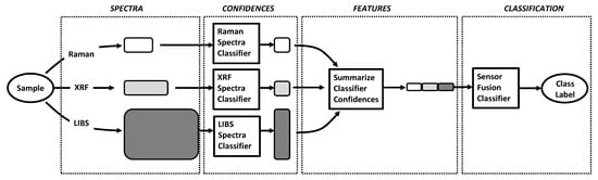
Figure 1.
Flow chart of the process used for analyzer data fusion. The three instruments collected spectra (Figure 2) from multiple locations on each soil pellet. These spectra are first classified using analyzer-specific classifiers, that output a set of confidence values that each spectrum belongs to each class. Then, the confidences from each analyzer-specific classifier are averaged and concatenated to generate a single vector for the sample. Finally, this vector is used as the input to the final data fusion classifier and a class label for the sample is generated.
The analyzer-specific classifiers were applied to the spectra generating Ns × C classifier confidences that the sample’s spectra belong to each of C classes, where the number of classes range from 2 to 6 depending on the classification schema (see Section 4, Table 1). In order to generate an input vector for the fusion classifier, the classifier confidences for each analyzer were averaged to produce a single 1 × C vector. These vectors were then concatenated to create a single vector that is 1 × 3C for the sample as an input to the final classifier. This feature input vector was classified by the fusion classifier and a class label assigned to the sample based on the class that generated the highest fusion-classifier confidence. Classification accuracy was estimated using leave-one-sample-out cross-validation. Each sample was in turn held out as a test sample and the remaining samples were used to train both the analyzer-specific and fusion classifiers.

Table 1.
Definition of the soil classification schemas and number of samples per class.
4. Results and Discussion
The classification schemas used for the three soil suites and the number of samples per class are show in Table 1. The New Mexico soils and military installation soils were classified based on the location from which the samples were collected. The New Hampshire soils were classified using two different schemas: location discrimination to separate Belmont and Lebanon samples, and intra-location discrimination to separate samples obtained from different layers of the three excavation pits at the Belmont Bean Hill site.
Examples of typical XRFS, RS, and LIBS spectra obtained during this study are presented in Figure 2. The extensive suites of XRFS, RS, and LIBS spectral data obtained for the natural soils and soil standards analyzed during this project are archived in the “JRPA Multisensor Project” folder on the Open Science Framework tool (https://osf.io/z3wgk/), together with other compositional information for these samples.
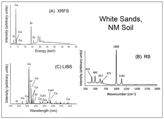
Figure 2.
Example of the XRFS, RS, and LIBS spectra used in this study for data fusion, in this case for the White Sands, NM soil. The XRFS spectrum (A) shows principally the presence of Ca, Sr, S, and Fe; the RS spectrum (B) shows the presence of documented bands for the vibrational modes of gypsum, CaSO4·2H2O [58]; and the LIBS broadband spectrum (C) showing mainly the presence of Ca and Sr, together with the minor levels of Si and Na. Note the presence of broad bands in the LIBS spectrum corresponding to the molecular bands of CaO, a species that is formed when O from the sample and the ambient atmosphere combines with the Ca in the soil.
4.1. Visualization
For visualization of the sample data in feature space, principal component analysis (PCA [59]) was applied to the fusion feature vectors (the 1 × 3C vectors used as input to the final classifier) to reduce their dimensionality. Such visualization can provide insight into the cause of any classification errors (e.g., the presence of outliers within a class, or the overlap of samples between classes). In order to plot the feature representation of the samples, the feature vectors are reduced to three or fewer dimensions even though the vectors are already of low dimensionality. The scores for the first three principal components are plotted for the New Mexico soils in Figure 3A and for the military installation soils in Figure 3B. While overlap between different classes in reduced-dimension feature space does not necessarily indicate classification will be poor, clear separation between the classes is indicative that classification accuracy will likely be high. For the New Mexico soils, the fused feature vectors demonstrate clear separation for all the classes except the Upper and Lower Socorro Canyon sites, suggesting that multiple analyzer data fusion will result in high classification accuracy. Similarly, for the military installation soils, the samples in each class generally show visual separation from the samples from other classes.
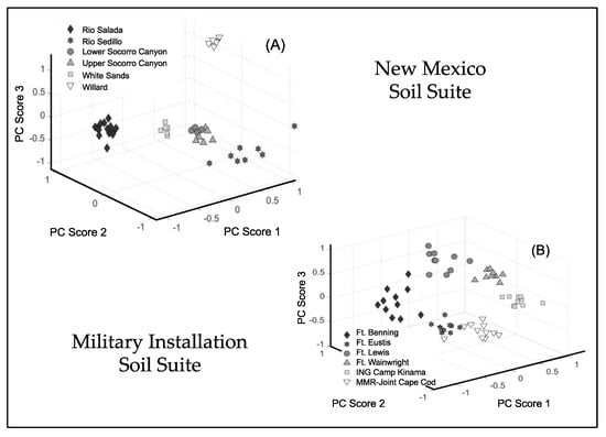
Figure 3.
Principal component score plots of the fusion feature vectors for the New Mexico soil suite (A) and the military installation soil suite (B).
For the New Hampshire soil suite, the samples separate clearly for the discrimination of the Lebanon and Belmont sampling locations (Figure 4A); however, a few class outliers exist for the intra-location samples at the Belmont site (Figure 4B). The outlier observed for Pit 2 is the deepest soil layer from this pit. Similarly, the two outliers observed for Pit 1 are the deepest and shallowest layers from this pit. Thus, as might be expected, soil depth has an impact on the measured spectra and may confound discrimination between sites.
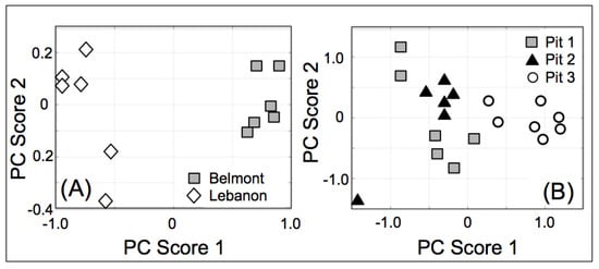
Figure 4.
Principal component score plots of the fusion feature vectors for the two New Hampshire locations (A) and at the three Belmont site pits (B).
4.2. PLSDA Loading Vectors
The multivariate data analysis approach utilized in this study outputs a set of loading vectors, which are coefficients that indicate the relative importance that each variable has on the predictive value of the PLSDA model. Before considering the results of individual PLSDA classification success and the relative merit of multianalyzer data fusion for the sample suites examined in this study, it is essential to understand the basis for discrimination. When loading values (in arbitrary units) are plotted against the relevant variables (i.e., energy, wavelength or Raman shift) associated with each analytical technique, the resulting plot has the appearance of a XRFS, LIBS or RS spectrum, except that the magnitude of the peaks or bands specifies how much of an effect it has on explaining the observed variation between the samples.
Examination of the loadings allows one to verify that the basis for classification is reasonable based on the anticipated composition of the soil samples. For example, the XRFS spectra for the New Mexico soils (Figure 5A) were classified primarily based on differences in the levels of Ca, Fe, and Sr with smaller contributions from S, K, Ti, Rb, and Ba. These results are consistent with the major and minor elements that can be detected by the XRFS analyzer and are present in the principal soil-forming silicate species, such as the feldspars and aluminosilicate clay minerals as well as various carbonates, oxides, and sulfates. Fe has the largest loading values for the XRFS classification task. This result is in accordance with the broad range of values found for Fe using the internally calibrated quantitation feature of the instrument. For example, the weight percentage of Fe in the New Mexico samples ranges over two orders of magnitude—from ~0.030% for the White Sands samples to ~3.4% for Sedillo Hill. The XRFS loadings profile for the military installation soil suite (Figure 5B) is similar to that obtained for the New Mexico soils, with some notable exceptions. K, Ca, Fe, Rb, Sr, and Ba are present in each XRFS loadings plot, though their relative significance differs, especially for Ca. Importantly, Pb lines play a major role in discrimination, possibly due to the presence of varying levels of Pb-contaminated soils at these firing range sites. Cu also has a notable impact on this PLSDA model.
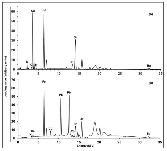
Figure 5.
Plot of loading vectors versus energy (keV) for the XRFS analysis of the New Mexico (A) and military installation (B) soil samples. Only the Kα lines are identified for the most significant loading values, except in the case of the Pb Lα and Lβ lines. Peaks associated with the Rh X-ray source and the broad Compton scattering peaks are also not labeled.
It is not surprising that the loadings associated with analysis of the soils from the six New Mexico locations using LIBS, which is especially sensitive to light elements, includes Li, Na, Mg, Al, and Si, in addition to K, Ca, Ti, Fe, and Sr (Figure 6A). Moisture content of the soils appears to also contribute to the discrimination since H and O also have appreciable loading values. While many of the same elements appear in the XRFS and LIBS plots for the New Mexico soils (Figure 5A and Figure 6A), labels for S and Rb are notably absent in the latter since the most intense emission lines for these elements appear at wavelengths greater than the 779 nm cut-off used to exclude argon lines from the chemometric analysis. The loadings plot for the PLSDA model built using the LIBS data for the military installation soil suite has significant values for Pb emission lines, a small contribution for Cu, as well as a similar profile of elements to that found with the New Mexico soils. Only loading values above an arbitrary threshold were labeled in the LIBS plots to simplify the graphical representation, but lines associated with several other elements common to soil such as Mn (403.1 nm) in the New Mexico soils and Cr (425.5 nm) in the military installation soils also have significant loading values.
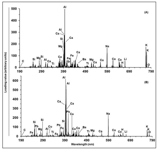
Figure 6.
Plot of loading vectors versus wavelength (nm) for the LIBS analysis of the New Mexico (A) and military installation (B) soil samples. The loading values that have the largest impact on the PLSDA model are labeled with the element associated with that emission line.
Though not displayed in a figure, the top loading vectors for the classification task associated with LIBS analysis carried out on soil samples from the Belmont and Lebanon, New Hampshire locations are, in order of importance, Ca, Al, Mg, Si, H, Fe, K, Ti, Na, C and O. The three Belmont location soil pits were distinguished on the basis of same elements in a similar order of relevance: Ca, Al, Mg, Si, H, Fe, Na, C, Ti, K and O. In these two cases, the contribution for the C line at 193.1 nm plays a more important role than for the other two soil suites, suggesting that varying amounts of organic matter aid in the discrimination. Likewise, the relative amount of moisture present in these samples contributed to the discrimination as evidenced by the comparably high loading value for the H line at 656.3 nm.
Soil is a complex mixture in different proportions of rocks fragments and minerals, organic materials, and moisture and gases, the Raman bands associated with the mineral components are expected to overlap. In addition, there is significant fluorescence associated with the organic components of soil. Since no attempt was made to remove the fluorescence background or to deconvolve overlapping bands, few peaks can be confidently identified, and the plots are not included in this paper. The only distinct loading for the New Mexico soils is the symmetric stretching mode of sulfate that appears at 1010 cm−1 [58]. This is the strongest of the sulfate stretching modes, as illustrated in the representative Raman spectrum of a gypsiferous sample from White Sands, NM (Figure 2). The military installation soils likewise do not have distinct peaks but rather show broad, unidentified, overlapping bands. The loading values for the Raman data have a dynamic range that is one or two orders of magnitude smaller than those found for the XRFS and LIBS classification tasks respectively. This suggests that the differences between the Raman spectra of soils from different locations is not as marked as for the data associated with the elemental analysis techniques.
4.3. Multianalyzer Data Fusion Results
The classification accuracy with each individual analyzer is compared to the accuracy achieved with data fusion for the New Mexico and military installation soil suites in Figure 7A. For the New Mexico soils, the classification accuracy for the individual analyzers ranges from 79. to 91% correct. Data fusion increases classification accuracy to 94% correct. For the military installation soils, classification relying on the RS spectra performs poorly with a classification accuracy of 64% correct. In contrast, classification using either the XRFS or LIBS spectra results in classification accuracy of >93% correct. Data fusion increases the classification accuracy to >98% correct. For both data sets, fusion increases classification accuracy over any of the individual instruments suggesting the benefit for assessing soils with multiple analyzers.
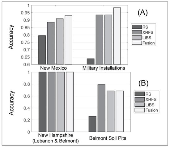
Figure 7.
Classification accuracy for the individual XRFS, RS, and LIBS analyzers and for three-instrument data fusion for (A) the New Mexico (left) and military installation soils (right) and (B) the New Hampshire Lebanon and Belmont and Lebanon locations (left) and the three Belmont location soil pits (right) described in Table 1.
Classification accuracy for the two New Hampshire soil schemas is shown in Figure 7B. As is expected from the principal component score plots (Figure 4), samples are perfectly discriminated in terms of the Lebanon and Belmont locations. This is true for each of the individual analyzers, thus their data fusion provides no additional benefit. For the within-location discrimination for the soil pits at the Belmont site, no benefit is observed for data fusion; however, this may be a result of the extremely poor classification accuracy with the RS spectra. This suggests that for multianalyzer data fusion to be beneficial, some minimum level of accuracy need be achieved by each instrument.
The potential for multianalyzer data fusion to correct classification errors is demonstrated in Figure 8 for the New Mexico soils. Four classification matrices are shown where the rows indicate the true class of the samples and the columns indicate the class label selected by the classification algorithm. The entries in the matrix, mi,j, are the percent of samples with the true label from row i and the classifier-selected label from column j. Thus, the diagonal entries are the percent of samples that were correctly classified, and off-diagonal entries demonstrate assignment errors made by the classifier.
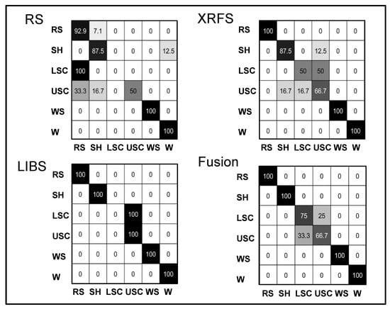
Figure 8.
Classification matrices for each individual analyzer for the New Mexico soil suite (RS, top left; XRFS, top right; LIBS, bottom left) and the data fusion (bottom right). Each row indicates the samples’ true class label and each column indicates the classifier label given to the samples analyzed from this class. Each entry is the percent (%) of samples with a row’s true label that were assigned a column’s label by the classifier. The diagonal entries indicate correctly classified samples and the off-diagonal entries indicate misclassifications. Location abbreviations are as follows: RS = Rio Salada, SH = Sedillo Hill, LSC = Lower Socorro Canyon, USC = Upper Socorro Canyon, WS = White Sands, and W = Willard.
As expected from the visualization in Figure 3, most classification errors for each analyzer occur between the Lower and Upper Socorro Canyon classes, where the geological similarity is high between soils at the two sites. None of the individual analyzers correctly classify the Socorro Canyon samples with greater than 60% accuracy. With data fusion, the classification accuracy of the Socorro Canyon samples is increased to 70% correct and other off-diagonal errors committed by single analyzer classification are eliminated.
For example, for the military installation soils, classification accuracy with data collected with the Raman analyzer is poor. In order to estimate the relative importance of each analyzer to the fusion classification, we considered the regression weights applied to each instrument’s data. In a trained PLSDA classifier, the regression weights are the values applied to the feature vector to estimate the confidence that a sample belongs to each class [60]. For each instrument, the magnitudes of the regression weights for the analyzer-specific features were pooled across the classes, and the probability density function (pdf) was estimated using kernel density estimation [59]. These pdfs provide a visualization of the range of regression weights applied to the features from each analyzer, with greater magnitudes indicating greater influence on the final classifier confidence.
Figure 9 shows the regression weight pdfs for each analyzer for the two data sets. For both data sets, the XRFS features are given the most weight. Further, the range of the pdf suggests that all of the XRFS features are used for classification (i.e., the pdf does not extend towards zero). In contrast, for the New Mexico soils, the means of the RS and LIBS pdfs are near zero suggesting that many of the RS and LIBS features are given little weight during classification. However, the long tails suggest that some of the features are given greater weight, and these are the features likely used for correcting errors committed by the XRFS classification.
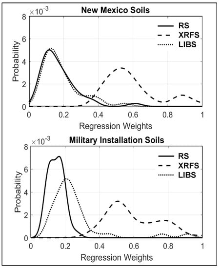
Figure 9.
Probability density functions (pdfs) for the PLSDA regression weights applied to the features for the RS, XRFS, and LIBS analyzers for the New Mexico soils (top) and military installation soils (bottom). The absolute value was taken of the regression weights since the magnitude, positive or negative, indicates degree of influence on the classification decision. The weights were also normalized to place the pdfs for the two data sets on the same scale.
With the military installation soils, for which the RS has poor classification accuracy, the mean of the pdf for features is close to zero, and the short tail suggests that few of these features have a large impact on the classification decision. By contrast, the LIBS features are farther from zero in general, suggesting greater influence on the classification decision. These results suggest the potential for the data fusion algorithm to be robust in classification scenarios in which an analyzer is unable to discriminate the classes well. During training, the PLSDA classifier determines the lack of reliable information in the features provided by the poorly performing instrument and applies lower weights to reduce the influence of this analyzer on the classifier decision. The hypothesis that data fusion may be robust despite poor individual analyzer classification performance is supported by the fusion results for the New Hampshire Belmont soil pits that, while showing no increase in classification accuracy with data fusion, demonstrate little negative impact from including the RS spectra.
5. Summary and Future Prospects
In this study, we analyzed 129 soil samples gathered from multiple locations in the United States using X-ray fluorescence spectroscopy, Raman spectroscopy, and laser-induced breakdown spectroscopy to evaluate the benefits of a data fusion approach for the compositional discrimination of geological materials. The data was obtained using commercially available, handheld chemical analyzers and subsequently processed using principal component analysis and partial least squares discriminant analysis. Classification models were built for individual instruments and the resulting confidences were combined and used as the input features for the data fusion classifier. The classification accuracy was evaluated utilizing leave-one-sample-out cross-validation. The basis for classification was assessed and found to be consistent with the presence of elements and species typically encountered in soil.
Our results, presented above for the two largest soil data sets, suggest the potential for combining the data from multiple analyzers to improve soil classification/discrimination. However, for both data sets, classification with the LIBS data alone provided >90% accuracy. The XRFS results were similarly very good, whilst classification accuracy based solely on the use of Raman spectra was notably poorer because RS observes molecular character by contrast to the elemental composition detected by LIBS and XRFS. Application of the three-analyzer/data fusion approach to other geological materials, such as a suite of minerals in which at least some samples display more distinctive Raman bands and less fluorescence than soil, is necessary to better judge the utility of this methodology. In general, additional testing with data sets for which classification with individual analyzers is poor might provide greater insight into the value and limits of data fusion for improving classification accuracy through error correction. While data fusion appears robust even though there was poor discrimination for one of the individual analyzers, as observed for the Belmont soil pit discrimination results, an assessment of data fusion for poor performance by one or more analyzers would inform the minimum level of performance necessary with each instrument in order to benefit from fusion of their respective spectral data streams.
Author Contributions
All authors contributed to the effort, with contributions as follows: Conceptualization and Writing—R.R.H., C.S.T., & R.S.H.; Methodology—R.R.H. & C.S.T.; Sample Acquisition—J.M.H.H., J.B.H., J.L.C.; R.S.H., R.R.H., & J.R.P.; Field and Laboratory Analysis—R.R.H., R.S.H., J.R.P., K.A.H., J.B.H., J.M.H.H., & J.L.C.; Data analysis & Visualization—C.S.T.; Project Administration—J.R.P.; and Funding Acquisition—J.R.P., R.S.H., & R.R.H. All authors have read and agreed to the published version of the manuscript.
Funding
This research was funded by the USACE Engineer Research & Development Center under contract number W913E518C0011 of 20 September 2018.
Conflicts of Interest
The authors declare no conflict of interest. The funding agency had no role in the design of the study, in the interpretation of data, or in the decision to publish the results.
References
- Hall, D.L.; Llinas, J. An introduction to multisensor data fusion. Proc. IEEE 1997, 85, 6–23. [Google Scholar] [CrossRef]
- Esteban, J.; Starr, A.; Willetts, R.; Hannah, P.; Bryanston-Cross, P. A review of data fusion models and architectures: Towards engineering guidelines. Neural Comput. Appl. 2005, 14, 273–281. [Google Scholar] [CrossRef]
- Luo, R.C.; Chang, C.C.; Lai, C.C. Multisensor fusion and integration: Theories, applications, and its perspectives. IEEE Sens. J. 2011, 11, 3122–3138. [Google Scholar] [CrossRef]
- Roussel, S.; Bellon-Maurel, V.; Roger, J.M.; Grenier, P. Fusion of aroma, FT-IR and UV sensor data based on the Bayesian inference. Application to the discrimination of white grape varieties. Chemom. Intell. Lab. Syst. 2003, 65, 209–219. [Google Scholar] [CrossRef]
- Biancolillo, A.; Bucci, R.; Magrì, A.L.; Magrì, A.D.; Marini, F. Data-fusion for multiplatform characterization of an Italian craft beer aimed at its authentication. Anal. Chim. Acta 2014, 820, 23–31. [Google Scholar] [CrossRef]
- Borràs, E.; Ferré, J.; Boqué, R.; Mestres, M.; Aceña, L.; Busto, O. Data fusion methodologies for food and beverage authentication and quality assessment—A review. Anal. Chim. Acta 2015, 891, 1–14. [Google Scholar] [CrossRef] [PubMed]
- Deneckere, A.; De Vries, L.; Vekemans, B.; Van de Voorde, L.; Ariese, F.; Vincze, L.; Moens, L.; Vandenabeele, P. Identification of inorganic pigments used in porcelain cards based on fusing Raman and X-ray fluorescence (XRF) data. Appl. Spectrosc. 2011, 65, 1281–1290. [Google Scholar] [CrossRef]
- Donais, M.K.; George, D.; Duncan, B.; Wojtas, S.M.; Daigle, A.M. Evaluation of data processing and analysis approaches for fresco pigment studies by portable X-ray fluorescence spectrometry and portable Raman spectroscopy. Anal. Methods 2011, 3, 1061–1071. [Google Scholar] [CrossRef]
- Wiens, R.C.; Sharma, S.K.; Thompson, J.; Misra, A.; Lucey, P.G. Joint analyses by laser-induced breakdown spectroscopy (LIBS) and Raman spectroscopy at stand-off distances. Spectrochim. Acta A 2005, 61, 2324–2334. [Google Scholar] [CrossRef]
- Khajehzadeh, N.; Haavisto, O.; Koresaar, L. On-stream mineral identification of tailing slurries of an iron ore concentrator using data fusion of LIBS, reflectance spectroscopy and XRF measurement techniques. Miner. Eng. 2017, 113, 83–94. [Google Scholar] [CrossRef]
- Xu, D.; Zhao, R.; Li, S.; Chen, S.; Jiang, Q.; Zhou, L.; Shi, Z. Multi-sensor fusion for the determination of several soil properties in the Yangtze River Delta, China. Eur. J. Soil Sci. 2019, 70, 162–173. [Google Scholar] [CrossRef]
- Desta, F.; Buxton, M.; Jansen, J. Data fusion for the prediction of elemental concentrations in polymetallic sulphide ore using mid-wave infrared and long-wave infrared reflectance data. Minerals 2020, 10, 235. [Google Scholar] [CrossRef]
- Gibbons, E.; Léveillé, R.; Berlo, K. Data fusion of laser-induced breakdown and Raman spectroscopies: Enhancing clay mineral identification. Spectrochim. Acta B 2020, 170, 105905. [Google Scholar] [CrossRef]
- Ahmed, N.; Ahmed, R.; Rafiqe, M.; Baig, M.A. A comparative study of Cu–Ni alloy using LIBS, LA-TOF, EDX, and XRF. Laser Part. Beams 2017, 35, 1–9. [Google Scholar] [CrossRef]
- Akhlaghi, I.A.; Haghighi, M.S.; Kahrobaee, S.; Hojati, M. Prediction of chemical composition and mechanical properties in powder metallurgical steels using multi-electromagnetic nondestructive methods and a data fusion system. J. Magn. Magn. Mater. 2020, 498, 166246. [Google Scholar] [CrossRef]
- Zhang, J. Multi-source remote sensing data fusion: Status and trends. Int. J. Image Data Fusion 2010, 1, 5–24. [Google Scholar] [CrossRef]
- Du, P.; Liu, S.; Xia, J.; Zhao, Y. Information fusion techniques for change detection from multi-temporal remote sensing images. Inf. Fusion 2013, 14, 19–27. [Google Scholar] [CrossRef]
- Shen, H.; Meng, X.; Zhang, L. An integrated framework for the spatio–temporal–spectral fusion of remote sensing images. IEEE Trans. Geosci. Remote 2016, 54, 7135–7148. [Google Scholar] [CrossRef]
- Rasti, B.; Ghamisi, P. Remote sensing image classification using subspace sensor fusion. Inf. Fusion 2020, 64, 121–130. [Google Scholar] [CrossRef]
- Kam, M.; Zhu, X.; Kalata, P. Sensor fusion for mobile robot navigation. Proc. IEEE 1997, 85, 108–119. [Google Scholar] [CrossRef]
- Luo, R.C.; Chang, C.C. Multisensor fusion and integration: A review on approaches and its applications in mechatronics. IEEE Trans. Industr. Inform. 2011, 8, 49–60. [Google Scholar] [CrossRef]
- Cremer, F.; Schutte, K.; Schavemaker, J.G.; den Breejen, E. A comparison of decision-level sensor-fusion methods for anti-personnel landmine detection. Inf. Fusion 2001, 2, 187–208. [Google Scholar] [CrossRef]
- Moros, J.; Laserna, J.J. New Raman–laser-induced breakdown spectroscopy identity of explosives using parametric data fusion on an integrated sensing platform. Anal. Chem. 2011, 83, 6275–6285. [Google Scholar] [CrossRef] [PubMed]
- Hoehse, M.; Paul, A.; Gornushkin, I.; Panne, U. Multivariate classification of pigments and inks using combined Raman spectroscopy and LIBS. Anal. Bioanal. Chem. 2012, 402, 1443–1450. [Google Scholar] [CrossRef]
- Klein, L.A. Sensor and Data Fusion: A Tool for Information Assessment and Decision Making; SPIE Press: Bellingham, WA, USA, 2004; 346p. [Google Scholar]
- Mahmood, H.S.; Hoogmoed, W.B.; van Henten, E.J. Sensor data fusion to predict multiple soil properties. Precis. Agric. 2012, 13, 628–645. [Google Scholar] [CrossRef]
- Sorak, D.; Herberholz, L.; Iwascek, S.; Altinpinar, S.; Pfeifer, F.; Siesler, H.W. New developments and applications of handheld Raman, mid-infrared, and near-infrared spectrometers. Appl. Spectrosc. Rev. 2012, 47, 83–115. [Google Scholar] [CrossRef]
- Pellegrino Vidal, R.B.; Ibañez, G.A.; Escandar, G.M. Advantages of data fusion: First multivariate curve resolution analysis of fused liquid chromatographic second-order data with dual diode array-fluorescent detection. Anal. Chem. 2018, 89, 3029–3035. [Google Scholar] [CrossRef]
- Casian, T.; Farkas, A.; Ilyés, K.; Démuth, B.; Borbás, E.; Madarász, L.; Rapi, Z.; Farkas, B.; Balogh, A.; Domokos, A.; et al. Data fusion strategies for performance improvement of a process analytical technology platform consisting of four instruments: An electrospinning case study. Int. J. Pharm. 2019, 567, 118473. [Google Scholar] [CrossRef]
- Taggart, J.E.; Lindsay, J.R.; Scott, B.A.; Vivit, D.V.; Bartel, A.J.; Stewart, K.C. Analysis of geologic materials by wavelength-dispersive X-ray fluorescence spectrometry. Methods Geochem. Anal. US Geol. Surv. Bull. 1987, 1770, E1–E19. [Google Scholar]
- Klockenkämper, R.; Von Bohlen, A. Elemental analysis of environmental samples by total reflection X-ray fluorescence: A review. X-Ray Spectrom. 1996, 25, 156–162. [Google Scholar] [CrossRef]
- von Bohlen, A. Total reflection X-ray fluorescence and grazing incidence X-ray spectrometry—Tools for micro-and surface analysis. A review. Spectrochim. Acta B 2009, 64, 821–832. [Google Scholar] [CrossRef]
- Kneipp, K.; Kneipp, H.; Itzkan, I.; Dasari, R.R.; Feld, M.S. Ultrasensitive chemical analysis by Raman spectroscopy. Chem. Rev. 1999, 99, 2957–2976. [Google Scholar] [CrossRef] [PubMed]
- Efremov, E.V.; Ariese, F.; Gooijer, C. Achievements in resonance Raman spectroscopy: Review of a technique with a distinct analytical chemistry potential. Anal. Chim. Acta 2008, 606, 119–134. [Google Scholar] [CrossRef]
- Rostron, P.; Gaber, S.; Gaber, D. Raman spectroscopy, review. Int. J. Eng. Res. 2016, 6, 50–64. [Google Scholar]
- Lee, Y.I.; Song, K.; Sneddon, J. Laser-Induced Breakdown Spectrometry; Nova Publishers: Hauppauge, NY, USA, 2000; 178p. [Google Scholar]
- Miziolek, A.W.; Palleschi, V.; Schechter, I. (Eds.) Laser Induced Breakdown Spectroscopy; Cambridge University Press: Cambridge, UK, 2006; 620p. [Google Scholar] [CrossRef]
- Singh, J.P.; Thakur, S.N. (Eds.) Laser-Induced Breakdown Spectroscopy, 2nd ed.; Elsevier: Amsterdam, The Netherlands, 2020; 620p. [Google Scholar]
- Hahn, D.W.; Omenetto, N. Laser-induced breakdown spectroscopy (LIBS), part I: Review of basic diagnostics and plasma–particle interactions: Still-challenging issues within the analytical plasma community. Appl. Spectrosc. 2010, 64, 335A–366A. [Google Scholar] [CrossRef]
- Hahn, D.W.; Omenetto, N. Laser-induced breakdown spectroscopy (LIBS), part II: Review of instrumental and methodological approaches to material analysis and applications to different fields. Appl. Spectrosc. 2012, 66, 347–419. [Google Scholar] [CrossRef]
- Cremers, D.A.; Radziemski, L.J. Handbook of Laser-Induced Breakdown Spectroscopy; Wiley: New York, NY, USA, 2013; 281p. [Google Scholar] [CrossRef]
- Musazzi, S.; Perini, U. (Eds.) Laser Induced Breakdown Spectroscopy; Springer: Berlin/Heidelberg, Germany, 2014; 564p. [Google Scholar] [CrossRef]
- McMillan, N.J.; Harmon, R.S.; De Lucia, F.C.; Miziolek, A.M. Laser-induced breakdown spectroscopy analysis of minerals: Carbonates and silicates. Spectrochim. Acta B 2007, 62, 1528–1536. [Google Scholar] [CrossRef]
- Gottfried, J.L.; Harmon, R.S.; De Lucia, F.C.; Miziolek, A.W. Multivariate analysis of laser-induced breakdown spectroscopy chemical signatures for geomaterial classification. Spectrochim. Acta B 2009, 64, 1009–1019. [Google Scholar] [CrossRef]
- Harmon, R.S.; Remus, J.; McMillan, N.J.; McManus, C.; Collins, L.; Gottfried, J.L.; DeLucia, F.C.; Miziolek, A.W. LIBS analysis of geomaterials: Geochemical fingerprinting for the rapid analysis and discrimination of minerals. Appl. Geochem. 2009, 24, 1125–1141. [Google Scholar] [CrossRef]
- Harmon, R.S.; Hark, R.R.; Throckmorton, C.S.; Rankey, E.C.; Wise, M.A.; Somers, A.M.; Collins, L.M. Geochemical fingerprinting by handheld laser-induced breakdown spectroscopy. Geostand. Geoanalytical Res. 2017, 41, 563–584. [Google Scholar] [CrossRef]
- Harmon, R.S.; Throckmorton, C.S.; Hark, R.R.; Gottfried, J.L.; Wörner, G.; Harpp, K.; Collins, L. Discriminating volcanic centers with handheld laser-induced breakdown spectroscopy (LIBS). J. Archaeol. Sci. 2018, 98, 112–127. [Google Scholar] [CrossRef]
- Ciucci, A.; Palleschi, V.; Rastelli, S.; Barbini, R.; Colao, F.; Fantoni, R.; Palucci, A.; Ribezzo, S.; Van der Steen, H.J.L. Trace pollutants analysis in soil by a time-resolved laser-induced breakdown spectroscopy technique. Appl. Phys. B 1996, 63, 185–190. [Google Scholar] [CrossRef]
- Essington, M.E.; Melnichenko, G.V.; Stewart, M.A.; Hull, R.A. Soil metals analysis using laser-induced breakdown spectroscopy (LIBS). Soil Sci. Soc. Am. J. 2009, 73, 1469–1478. [Google Scholar] [CrossRef]
- Unnikrishnan, V.K.; Nayak, R.; Aithal, K.; Kartha, V.B.; Santhosh, C.; Gupta, G.P.; Suri, B.M. Analysis of trace elements in complex matrices (soil) by Laser Induced Breakdown Spectroscopy (LIBS). Anal. Methods 2013, 5, 1294–1300. [Google Scholar] [CrossRef]
- Senesi, G.S.; Harmon, R.S.; Hark, R.R. Field-portable and handheld laser-induced breakdown spectroscopy: Historical review, current status and future prospects. Spectrochim. Acta B 2020, 175, 106013. [Google Scholar] [CrossRef]
- Ramos, P.M.; Ruisánchez, I.; Andrikopoulos, K.S. Micro-Raman and X-ray fluorescence spectroscopy data fusion for the classification of ochre pigments. Talanta 2008, 75, 926–936. [Google Scholar] [CrossRef]
- Sánchez-Esteva, S.; Knadel, M.; Kucheryavskiy, S.; de Jonge, L.W.; Rubæk, G.H.; Hermansen, C.; Heckrath, G. Combining laser-induced breakdown spectroscopy (LIBS) and visible near-infrared spectroscopy (Vis-NIRS) for soil phosphorus determination. Sensors 2020, 20, 5419. [Google Scholar] [CrossRef]
- Brereton, R.G.; Lloyd, G.R. Partial least squares discriminant analysis: Taking the magic away. J. Chemom. 2014, 28, 213–225. [Google Scholar] [CrossRef]
- Wold, S.; Sjöström, M.; Eriksson, L. PLS-regression: A basic tool of chemometrics. Chemom. Intell. Lab. Syst. 2001, 58, 109–130. [Google Scholar] [CrossRef]
- De Jong, S. SIMPLS: An alternative approach to partial least squares regression. Chemom. Intell. Lab. Syst. 1993, 18, 251–263. [Google Scholar] [CrossRef]
- Davies, L.; Gather, U. The identification of multiple outliers. J. Am. Stat. Assoc. 1993, 88, 782–792. [Google Scholar] [CrossRef]
- Jehlička, J.; Vitek, P.; Edwards, H.G.M.; Hargreaves, M.D.; Čapoun, T. Fast detection of sulphate minerals (gypsum, anglesite, baryte) by a portable Raman spectrometer. J. Raman Spectrosc. 2008, 40, 1082–1086. [Google Scholar] [CrossRef]
- Bishop, C.M. Pattern Recognition and Machine Learning; Springer: Berlin/Heidelberg, Germany, 2006; 738p. [Google Scholar]
- Mehmood, T.; Liland, K.H.; Snipen, L.; Sæbø, S. A review of variable selection methods in Partial Least Squares Regression. Chemom. Intell. Lab. Syst. 2012, 118, 62–69. [Google Scholar] [CrossRef]
Publisher’s Note: MDPI stays neutral with regard to jurisdictional claims in published maps and institutional affiliations. |
© 2020 by the authors. Licensee MDPI, Basel, Switzerland. This article is an open access article distributed under the terms and conditions of the Creative Commons Attribution (CC BY) license (http://creativecommons.org/licenses/by/4.0/).