Abstract
Synthetic aperture radar (SAR) images have been used in many studies for ship detection because they can be captured without being affected by time and weather. In recent years, the development of deep learning techniques has facilitated studies on ship detection in SAR images using deep learning techniques. However, because the noise from SAR images can negatively affect the learning of the deep learning model, it is necessary to reduce the noise through preprocessing. In this study, deep learning vessel detection was performed using preprocessed SAR images, and the effects of the preprocessing of the images on deep learning vessel detection were compared and analyzed. Through the preprocessing of SAR images, (1) intensity images, (2) decibel images, and (3) intensity difference and texture images were generated. The M2Det object detection model was used for the deep learning process and preprocessed SAR images. After the object detection model was trained, ship detection was performed using test images. The test results are presented in terms of precision, recall, and average precision (AP), which were 93.18%, 91.11%, and 89.78% for the intensity images, respectively, 94.16%, 94.16%, and 92.34% for the decibel images, respectively, and 97.40%, 94.94%, and 95.55% for the intensity difference and texture images, respectively. From the results, it can be found that the preprocessing of the SAR images can facilitate the deep learning process and improve the ship detection performance. The results of this study are expected to contribute to the development of deep learning-based ship detection techniques in SAR images in the future.
1. Introduction
Ship detection is a critical maritime management technology and encompasses fields such as the investigation of illegal fishing areas, oil spill detection, maritime traffic management, and national defense [1,2,3,4]. Currently, to monitor ships, the International Maritime Organization mandates all international ships over 300 tons, all domestic passenger ships, and cargo ships over 500 tons to install an automatic identification system (AIS). However, if the density of a ship is high, the AIS signal may be affected by interference, which reduces the effective reception distance, and may not be received by other ships or base stations [5]. In addition, when AIS is deliberately turned off by a fishing ship, it is impossible to locate the ship.
Satellite images can be used as an alternative for detecting ships in the sea. If satellite images are used, most ships in vast water bodies can be effectively detected regardless of the operation of the AIS. There are two main types of sensors for capturing satellite images: an optical sensor, which is a passive sensor, and a synthetic aperture radar (SAR) sensor, which is an active sensor. The optical sensor generates an image by detecting sunlight reflected from an object. Because the optical sensor uses the visible color spectrum to capture images, ships in images captured by an optical sensor can be easily identified by a person. However, owing to the requirement of sunlight, images can only be captured by an optical sensor during daytime. Further, high-quality images cannot be captured if the weather conditions are bad, even during daytime. In contrast, because the SAR sensor generates an image by emitting a signal from the sensor and detecting the reflected signal from an object, images can be generated even at night [2,6]. In addition, because the emitted signal for ship detection is not affected by weather conditions, it is useful for ship detection research [2,7,8].
Recently, various ship detection studies focused on the deep learning model structure rather than improving the quality of images [9,10,11,12]. In contrast, the present study focuses on the preprocessing technique of SAR images to improve ship detection performance. First, the value unit of the SAR images was converted to decibels to present a normal distribution of the values. Then, noise in the images that can interfere with ship identification was reduced by using a multi-looking technique and a median filter [13]. Moreover, for better contrast between the ship and the sea, images were created with only sea surface image data remaining. First, a median filter was used having a size sufficiently larger than the size of the ship in the images [13]. Noise in the entire image was reduced, and the contrast between the sea and the ship was increased by separating the filtered images from the existing SAR images. In addition to the increased contrast, it is expected that ships can be detected more easily by changing the state of the sea surface in all images. The preprocessed images were converted into training data and test data through visual analysis and comparison using Google Earth.
The purpose of this study is to detect ships in SAR images using deep learning. We used an M2Det [14] deep learning model for detecting ships in SAR images. To enhance detection accuracy, we proposed a preprocessing method for SAR images and compared its detection results to others from different preprocessed images. The ship detection performance was expressed in terms of precision, recall, and average precision (AP) [15,16,17]. By using the proposed preprocessing method, the trained M2Det deep learning model could achieve highest accuracy (95.55% AP).
Related Works
In SAR images, the locations of ships appear bright because of corner reflections [8,18]. In previous studies, they tried to detect ships based on pixel brightness. However, they often detected other bright objects, such as ship wake and islands, as ships [19,20,21]. To reduce this problem, Hwang et al. [22] proposed a SAR image preprocessing method. They applied multi-looking twice and used a median filter to reduce speckle noise in SAR images. They generated normalized intensity and texture images as a result of their proposed method [22]. Ref. [23] also applied a similar preprocessing method and demonstrated enhanced detection results. Our proposed preprocess method is mostly inspired by [22,23]. We created two images from the proposed preprocessing method. One is an intensity difference image and the other is a texture image. However, to avoid degrading detection performance due to reduced spatial resolution, we applied multi-looking only once.
2. Study Data
In this study, images captured by TerraSAR-X and COSMO-SkyMed (Constellation of Small Satellites for Mediterranean basin Observation) satellites were used to detect ships. TerraSAR-X is a German satellite that was successfully launched on June 15, 2007 and is a high-resolution SAR satellite using X-band microwaves. Three modes, namely, the Spotlight, ScanSAR, and StripMap, are supported. Because each mode has different observation widths and resolutions, a mode can be selected according to the purpose of the study. The Spotlight mode provides a 1 m resolution image for a 10 km observation width, and the StripMap mode provides a 3 m resolution image for a 30 km observation width. Finally, the ScanSAR mode provides a 16 m resolution image for a wide viewing width of 100 km. COSMO-SkyMed is a group of four satellites owned by Italy. Similar to TerraSAR-X, they support three modes: the Spotlight mode, ScanSAR mode, and StripMap mode. Among the three modes, the StripMap mode, which provides a 3 m resolution image, was used in this study. Therefore, most ships can be detected considerably well, except very small ships, and thus this mode is suitable for this study. Table 1 lists the details of the TerraSAR-X and COSMO-SkyMed SAR images used in this study. The parameters of each SAR image represent the average value of the images used. The pixel resolution in the flight direction of the TerraSAR-X image is approximately 2.4 m, and the pixel size in the observation direction is approximately 1.9 m. Furthermore, the COSMO-SkyMed image has approximately 2.1 m pixel resolution in both the flight direction and the observation direction. For polarization, both SAR images used the HH mode. In the co-polarization mode, HH polarization is known to have a higher contrast between sea and ship than VV polarization. Therefore, it was expected that this would yield a better ship detection performance [24]. TerraSAR-X used a total of four images, and these images were captured in Songdo, Korea, and the Kerch Strait between the Black Sea and the Azov Sea. COSMO-SkyMed used a total of 26 images, and those images were in Songdo, Korea, and Gyeongju, Korea.

Table 1.
Details of COSMO-SkyMed and TerraSAR-X images used in this study. SAR: synthetic aperture radar.
Figure 1 shows some of the SAR images used in this study. Figure 1e is an enlarged image of a part of an oil spill area in the Kerch Strait in November 2007. Mostly small ships are observed, and the sea surface on which the oil floats is calm. Figure 1f shows a small ship and a large ship together and a calm water surface. In Figure 1g,h, waves are swaying on the water surface, and small ships are observed. As shown in Figure 1, although the contrast between the values of the ship and the sea surface is large in both cases, the conditions of the sea surface and the size of the ship are different in each sea. Therefore, it is important to successfully detect large and small ships that exist at sea surface in various states.

Figure 1.
Intensity image of SAR image used in this study. (a) Kerch Strait captured by TerraSAR-X; (b) Songdo captured by TerraSAR-X; (c) Songdo captured by COSMO-SkyMed; (d) Gyeongju captured by COSMO-SkyMed; (e–h) zoomed in images of the red box region in (a–d).
3. Methods
Figure 2 shows the flow chart of this study, which is divided into (a) an input layer, which indicates an input image and (b) deep learning, in which ship detection learning is performed using a deep learning model. In this study, the SAR image was preprocessed in three different ways to compare the effect on the ship detection result of different training data used during the deep learning model training. An image set generated through each preprocessing is shown in Figure 2a. The first is the SAR intensity image without any preprocessing. In the second, a decibel image was generated by converting the unit of the SAR intensity image values to decibels. Because the intensity image shows a Rayleigh distribution, and the decibel image shows a normal distribution, it was predicted that the decibel image would yield better detection results than the intensity image. Finally, in the third, the intensity difference image and texture image were created. It was expected that the ship detection test results would be improved by enhancing the contrast between the ship and the sea surface through the two images and reducing occasions where other objects are confused with ships. The training data and test data were constructed using images generated by three different preprocessing methods. Figure 2b represents the deep learning model used for ship detection. M2Det was used as the object detection model for ship detection, and DenseNet [25] was used as the backbone network. By using M2Det, it was expected that ships of various sizes, from very small to very large ships, would be detected well. Furthermore, by using DenseNet as a backbone network instead of VGGNet [26] or ResNet [27], which are the backbone networks in the existing M2Det, features of all layers can be used rather than selecting specific layers on the network and extracting features. It was expected that the ship detection performance would be improved by doing this. Furthermore, by using RAdam [28] as the optimization function, stable learning could be performed regardless of the learning rate in all input image sets. After the deep learning model training was completed, the bounding boxes indicating the locations of ships and the confidence score for each bounding box were derived as the detection result.
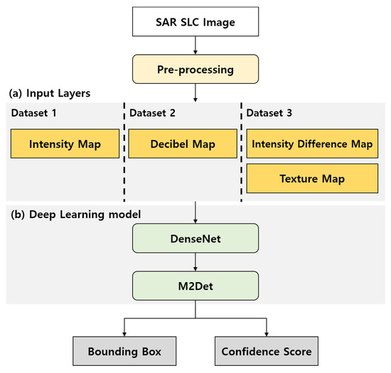
Figure 2.
Research flow chart. SLC: Single Look Complex. (a) Input layers; (b) Deep learning model.
3.1. SAR Image Preprocessing
Figure 3 shows a flow chart of the SAR image preprocessing performed to improve the ship detection performance using deep learning. Through preprocessing, the ship detection performance was expected to be improved by reducing the noise in the SAR images and increasing the contrast between the ship and the sea. As shown in Figure 3, the images used for comparison in this study were: (1) intensity image, (2) decibel image, and (3) intensity difference image and texture image. Unlike the intensity and decibel images, the intensity difference image and texture image were used in combination.
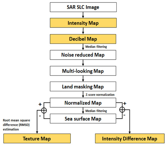
Figure 3.
Flow chart of proposed SAR image preprocessing in this study.
3.1.1. Decibel Conversion
It is known that a neural network is better optimized when the distribution of the input data follows a normal distribution during neural network training [29]. Therefore, in this study, the distribution of the values of the SAR images was first converted into a distribution similar to the normal distribution. The conversion process of the distribution of the data that are analyzed for actual data analysis is a frequently used technique [30]. In the case of SAR images, it can be converted to the distribution that approximates the normal distribution through log transformation [31,32]. In Figure 3, the decibel image indicates an image in which the intensity image is expressed in decibels through decibel conversion and can be generated using the following equation.
where x is a SAR intensity image, and y is a SAR intensity image converted into decibels.
3.1.2. Speckle Noise Reduction
In general, speckle noise exists in SAR images, and speckle noise is a factor that degrades the image quality. Therefore, the noise must be reduced before image analysis. In this study, noise in the image was reduced using a median filter and multi-looking technique [33]. First, median filtering was performed. If the median filter size is too large, the pixels of the ship in the image may be replaced by pixels of the sea. Therefore, the size of the filter should be determined based on the size of the ship. In addition, if the size of the ship becomes too small due to multi-looking, the ship may not be detected. Therefore, the number of looks in the multi-looking should be determined based on the size of the ship, such as the size of the median filter.
3.1.3. Land Masking
In the land area, because many objects, for example buildings and containers, can cause double scatterings, most land areas show a high backscattering coefficient on the image. Because a high backscattering coefficient can lead to false detection, many ship detection studies perform a land masking before ship detection [1,33,34]. In this study, a digital elevation model (DEM) of the Shuttle Radar Topography Mission (SRTM) with a 30 m resolution was used to mask the land area. To remove the land area from the SAR image using the DEM, the geometry of the image and the DEM were matched using intensity cross-correlation. However, reclaimed area after DEM was created still remain on image. To cover this area with DEM, we made a buffer area on the DEM, then removed it.
3.1.4. Image Normalization
As the average value of the input data deviates from 0, a bias may occur in a specific direction when the weight is updated, resulting in a slower learning speed [35]. Therefore, the training data should be normalized to uniformly train the weights and expedite the training process [35]. In this study, Z-score normalization was performed to normalize the input image, and the following equation was used:
where x indicates each SAR image, and μ and σ denote the mean and standard deviation of x, respectively. The learning of the neural network can be performed faster than prior to normalization by normalizing each image using Equation (2).
3.1.5. SAR Intensity Difference Image and Texture Image
To generate an intensity difference image and a texture image from the normalized image, sea surface values were extracted from the normalized image using a very large median filter [30]. In addition, to extract the sea surface values only, a median filter with a sufficiently large size of 81 × 81 was used based on the size of the ship on the image. The generated sea surface image was differentiated from the existing image where the ship appeared to create an intensity difference image, and a texture image was created by calculating the root mean square difference (RMSD). Through this, phenomena appearing at sea surface such as waves and ripples can be reduced, and at the same time, the contrast between the ship and the sea can be increased slightly.
3.2. Generation of Training and Validation Data
The size of SAR images is significantly large, and the typical size of a single image is several gigabytes. Therefore, a large amount of memory is required to learn an entire image during the training process. Due to insufficient memory of our graphics card, all 30 SAR images were divided into patches with a size of 320 × 320. Each patch image was overlapped by 20% to adjacent patch images to prevent ship objects from being cut, which would have resulted in them not being used for training and validation processes. As a result, we generated a total of 1160 patch images and divided them into training and test data in an 8:2 ratio. In other words, the numbers of images for the training process and the test process were 928 and 232, respectively. Furthermore, the entire training images were divided into a 3:1 ratio for cross-validation. In other words, the number of images for the training and validation dataset were 696 and 232, respectively.
In each patch image, the ground truth was generated using LabelImg [36], and visual analysis and Google Earth software were used to identify the ship on the image.
3.3. Training and Validation Method
In this study, the M2Det model was used for ship detection. Figure 4 shows the architecture of M2Det. M2Det uses a multi-level feature pyramid network (MLFPN) module to extract more fluent information from images. MLFPN consists of a thinned u-shape module (TUM), feature fusion module (FFM) and scale-wise feature aggregation module (SFAM) module. TUM utilizes various sizes of feature maps so that extract information from various size of objects efficiently. FFM concatenates features between TUMs and the backbone network to extract information from multi-levels. SFAM creates multi-level feature pyramid with features extracted from multi-level and multi-scale images. Lastly, M2Det detects objects from the multi-level feature pyramid using the same anchor boxes as in SSD (Single Shot multibox Detector) [37] deep learning model. The aspect ratios of the anchor box for object detection in the existing M2Det are . However, because the long part of the ship is considerably longer than the short part, some ships may not be detected if the original ratio is used in the case of a ship. Therefore, in this study, were used by adding a longer ratio to the existing anchor box. In implementation details, we used RAdam optimization and batch size was 4. In the MLFPN, we used 6 scales and 8 levels—the same as [14].
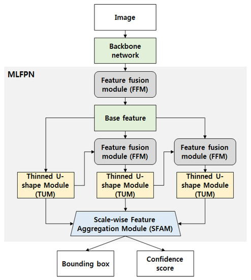
Figure 4.
Architecture of M2Det. MLFPN: multi-level feature pyramid network.
In general, the object detection model detects objects using features extracted through the backbone network, and VGGNet, ResNet, and DenseNet are mainly used as the backbone networks [37,38,39,40]. When VGGNet or ResNet is used as a backbone network, features of several layers are often fused to detect small objects [10,41]. However, DenseNet utilizes all of the features from the previous layer in each layer, it was found that the process of selecting a layer for feature fusion could be omitted and the features of the ships could be better extracted. Therefore, in this study, DenseNet was used as the backbone network of M2Det.
First, cross-validation was performed in each preprocessed dataset to get the best initial weight parameter. After set the initial weight, the deep learning model was trained using the entire training and validation set. When the entire training and validation set was used, six training processes were performed in each preprocessing method for choosing best learning rate, and the learning rate of each training was (0.005, 0.001, 0.0005, 0.0001, 0.00005, 0.00001). In addition, to increase robustness of the model, zoom in/out, cropping, and horizontal flipping were used, and values of all images were normalized to the [0, 1] range before being used.
After the training is completed, the test results were expressed in terms of AP, precision, and recall. AP is the bottom area of the precision and recall graphs and can be expressed by the following equation:
where r indicates the recall and p(r) indicates the precision at each recall. Furthermore, the precision and recall are defined as follows:
where TP is the number of events where the model predicted a true value as true, FN is the number of events where the model predicted a true value as false, and FP is the number of events where the model predicted a non-true value as true. Therefore, the precision represents the ratio of the number of actual true values to the number of true values that the model predicted as true, and the recall represents the ratio of the number of true values that the model predicted as true to the number of actual true values. In addition, because precision and recall depend on the threshold value, the critical success index (CSI) was used to determine the optimal threshold value and is defined as follows [42,43]:
4. Results
4.1. SAR Preprocessing Result
First, the SAR image was converted into decibels through decibel conversion, thereby converting the distribution of values to a normal distribution. Figure 5 shows a magnetized intensity image of the red box in Figure 1e (1). Figure 5b depicts an intensity decibel image converted from Figure 5a using Equation (4). Figure 5c,d shows the histograms of Figure 5a,b, respectively. As illustrated in Figure 5d, the SAR image showing the Rayleigh distribution shows a normal distribution through the decibel conversion. Furthermore, before the decibel conversion, the distribution band of the values was widely distributed from tens of thousands to hundreds of thousands, but after the decibel conversion, the distribution band was significantly narrowed down to tens. Because of these changes, it can be expected that the weights will be learned in a balanced way during the training process [35].
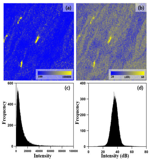
Figure 5.
(a) Magnified intensity image of the red box in Figure 1e (1); (b) intensity decibel image of (a); (c) histogram of (a); (d) histogram of (b).
After a decibel image was created, median filtering and multi-looking were performed to reduce speckle noise in the image. To prevent the disappearance of small ships owing to their small number of pixels and median filtering, the size of the median filter was selected to be 3 × 3, which is the minimum size. Moreover, to prevent a ship from becoming a dot owing to its small size, only two looks were performed in the range and azimuth directions. Figure 6 shows the effect of speckle noise reduction by using a median filter and multi-looking. Figure 6a,b shows an intensity decibel image before and after speckle noise reduction, respectively. Furthermore, Figure 6c,d show the histograms of Figure 6a,b, respectively. The difference is barely noticeable because the sizethe median filter was 3 × 3. However, as shown in Figure 6d, it can be observed that the noise components of the sea surface are reduced by speckle noise reduction.
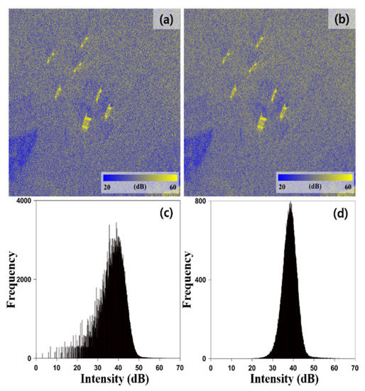
Figure 6.
(a) Magnified intensity decibel image of the red box in Figure 1e (2); (b) the same image with reduced speckle noise; (c) a histogram of (a); (d) a histogram of (b).
Subsequently, land masking was performed using the DEM with a resolution of 30 m. However, because some artifacts, such as bridges built after the DEM were created, do not appear in the DEM, the artifacts cannot be eliminated. To cover these area, we added buffer area at the edge of DEM. The DEM and the SAR image were matched using the intensity cross-correlation and then overlapping areas were removed (Figure 7).
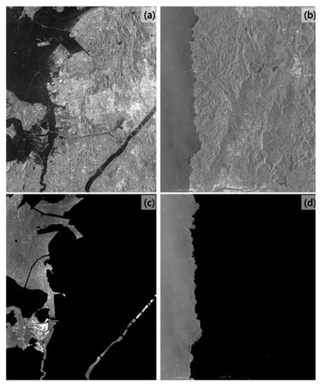
Figure 7.
(a,b) COSMO-SkyMed SAR image; (c) the land masking result of (a); (d) land masking result of (b).
Images were normalized after masking the land in the SAR image. After this, sea surface images were generated from the normalized images. If median filters are applied more than twice the size of a ship, the shape of the ship will almost disappear in the images and only the smoothed sea surface remains [33]. Therefore, the size of the filter must be determined by considering the size of the ships [33]. In the images used in this study, the size of the ship was about 10 to 40 pixels. Therefore, we designed the filter with a size of 81 × 81 based on the largest ships. Figure 8a–c shows the normalized images, and Figure 8d–f shows the sea surface images generated through median filtering from Figure 8a–c, respectively. As shown in Figure 8d–f, it can be observed that only the shape of the sea surface remained in the sea surface image, and very little influence from the ship was found.
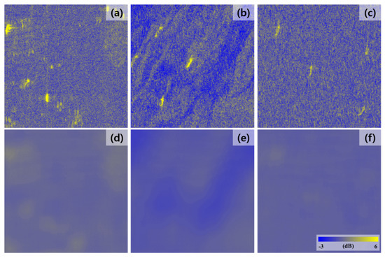
Figure 8.
(a–c) Normalized intensity image; (d–f) sea surface images generated from (a–c) in the order of (b,d,f).
Simple difference and RMSD calculations were performed using normalized intensity images and sea surface images to generate intensity difference images and texture images. Figure 9a,b shows the intensity difference image and the texture image, respectively, and Figure 9c,d depicts the histograms of Figure 9a,b, respectively. The red boxes in Figure 9c,d indicate the distribution band of ship pixel values. Although the distribution bands of ship pixel values in the intensity difference image and the texture image show similar levels, the overall distributions of the images are different. Therefore, by using the intensity difference image and the texture image, it is possible to create the same effect as if the same ship was captured at the sea surface under different conditions. Furthermore, it could be made more insensitive to the distribution of sea surface values in ship detection by using the intensity difference image and the texture image simultaneously.
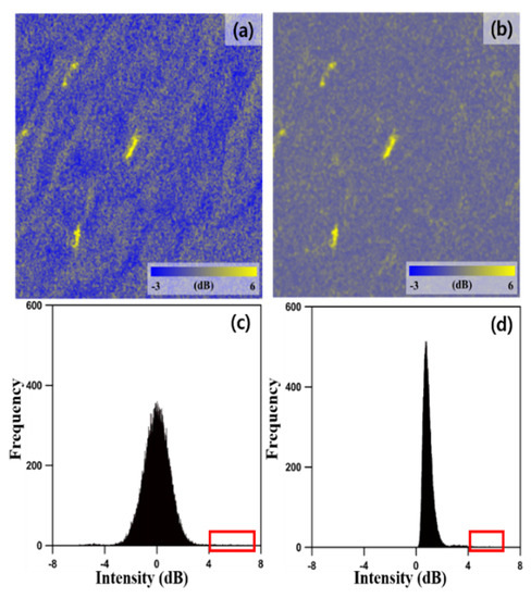
Figure 9.
(a) Intensity difference image; (b) texture image (c) histogram of the intensity difference image; (d) histogram of the texture image. The red box in the histogram indicates the distribution band of the ship pixel values.
4.2. Ship Detection Result
For verifying the effect of the proposed processing method, the model was trained in three ways using (1) SAR intensity images, (2) decibel images, (3) intensity difference, and texture images, respectively. These models were trained using 928 images that consisted of training and validation datasets. To obtain the evaluation results, 232 test images were used. In Figure 10, Figure 11 and Figure 12, the test results of the trained model using each training image are expressed in terms of the recall, precision, and CSI, according to the threshold. We decided the optimal threshold at the maximum CSI in each test result. As a result, the proposed model has the lowest optimal threshold. It means when training preprocessed images using our proposed method, the deep learning model can differentiate ship objects better.
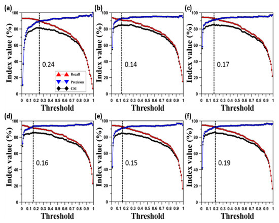
Figure 10.
Test results according to the threshold of the model using intensity images. The red graph represents recall, blue graph represents precision, and black graph represents the critical success index. Learning rates were (a) 0.005; (b) 0.001; (c) 0.0005; (d) 0.0001; (e) 0.00005; (f) 0.00001. The dotted line represents the critical value at the maximum critical success index.
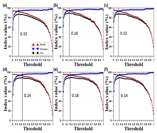
Figure 11.
Test results according to the threshold of the model using decibel images. The red graph represents recall, blue graph represents precision, and black graph represents the critical success index. Learning rates were (a) 0.005; (b) 0.001; (c) 0.0005; (d) 0.0001; (e) 0.00005; (f) 0.00001. The dotted line represents the critical value at the maximum critical success index.
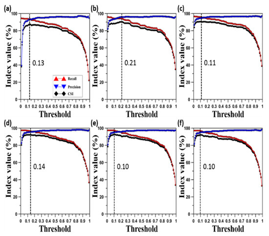
Figure 12.
Test results according to the threshold of the model using intensity difference and texture images. The red graph represents recall, blue graph represents precision, and black graph represents the critical success index. Learning rates were (a) 0.005; (b) 0.001; (c) 0.0005; (d) 0.0001; (e) 0.00005; (f) 0.00001. The dotted line represents the critical value at the maximum critical success index.
Table 2 lists the precision, recall, and AP when the optimal threshold value was used for each model. For the model trained using the intensity images, the results were worse than those of the model trained using the preprocessed image in terms of recall, precision, and AP. The precision values of the models trained using the decibel images, intensity difference images, and texture images were similar. However, it can be found that the recall values of the models trained using the intensity difference and texture images were different from the recall value of the model trained using the decibel image by up to 3%. This means that the percentage of undetected ships decreased by 3%. Similarly, when the AP values were compared, it was found that the AP values of the models trained using the intensity difference and texture images were higher by up to 3%. Therefore, when preprocessed images were used in the training process, the ship detection performance was improved. In particular, the preprocessing method proposed in this study was found to be effective in improving the deep training process.
Table 2.
Recall, precision, average precision (AP) at the optimal threshold of each model according to the learning rate. The values in boldface indicate the highest AP index in the corresponding set of images.
Figure 13 shows some of the results when the ships were detected by the learning model having the highest AP in each set of the training images and the optimum threshold value. In Figure 13b, it can be observed that small ships that exist in the sea with strong sea backscatter were detected well. Furthermore, from Figure 13c, it can be observed that ships were distinctly detected despite the presence of a sediment area and a strong side-lobe effect.
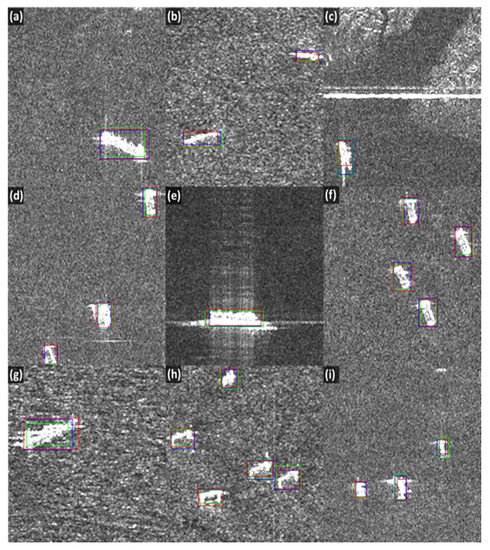
Figure 13.
Result of detecting a ship by applying the optimal threshold of each input image in the model with the highest AP index in each training image. Green box: intensity image, blue box: decibel image, and red box: intensity difference and texture image; (a,b,d,f–i) ships on the sea with sea backscattering effect; (c,e) ships with strong side-lobe effect.
Figure 14 shows the false ship detections in each detection result. False detection occurred in the ship wakes. This is because the images with the ship wake accounted for only 4% of the total learning images, thereby the learning of the ship wake was not well performed. However, even in such cases, the intensity difference and texture image rarely recognized ship wake as ships. In Figure 14e, it can be observed that false detections occurred in all images. When several ships were very close to each other, it was difficult to distinguish them from the image; therefore, those ships were recognized as a single ship.
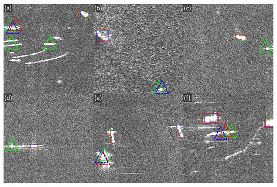
Figure 14.
False detection results when the optimal threshold of each input image was applied in the model with the highest AP index in the training image (a–f). Green box: intensity image, blue box: decibel image, red box: intensity difference/texture image, and dotted triangle: false detection.
Figure 15 shows the result of undetected ships in each detection result. The intensity image without preprocessing shows the largest number of undetected ships. The preprocessed image mainly shows false positives in small ships of 15 pixels or less. It can be determined from the detection results that more ships were detected when using the intensity difference and texture images than when using the decibel image.
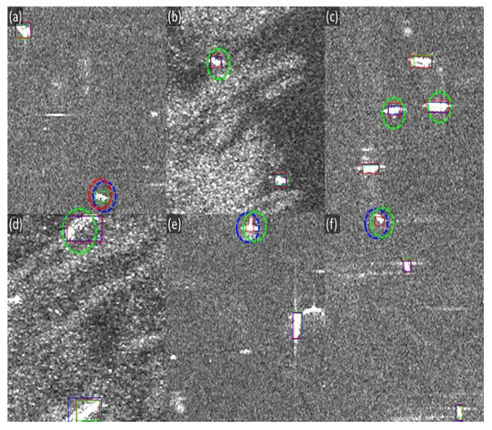
Figure 15.
Undetected ships when the optimal threshold of each input image was applied in the model with the highest AP index in the training image (a–f). Green box: intensity image, blue box: decibel image, red box: intensity difference/texture image, and dotted ovals: undetected cases.
Table 3 shows undetected ships according to size. The size of the ship is taken as the longer side between the width and the length of the ship, and it can be found that a ship with a size of 30–50 pixels accounts for approximately 50% of the total number of ships. The intensity image showed the largest number of undetected cases in most ships regardless of size. Although the number of undetected cases in the decibel image is less than that in the intensity image, undetected cases were found even for large ships, indicating that this image is unstable. In contrast, using the intensity difference and texture images, it can be found that the number of undetected cases is certainly less than with other images. From these results, it can be found that when the preprocessing method proposed in this study is used, more ships can be detected compared to when the preprocessing method is not used.
Table 3.
Number of undetected cases according to ship size. The size of the ship is the number of pixels of the longer side between the width and length of the ship. The number in the preprocessing column indicates the number of undetected ships in each size.
5. Conclusions
In this study, deep learning was used to detect ships from X-band SAR images. Furthermore, to further improve the ship detection performance, a preprocessing method was proposed to reduce the noise in the SAR image and increase the contrast between the sea and the ship. In addition, to verify the performance of the preprocessing method proposed in this study, both the intensity image without preprocessing and the intensity image after conversion to the decibel image were used as training images, and the test results were compared.
The best detection performance was obtained when the intensity image with a learning rate of 0.001 was used and when the decibel image and intensity difference/texture image combination with a learning rate of 0.00005 was used. The highest AP values of the intensity images, decibel images, and intensity difference/texture images were 89.78%, 92.34%, and 95.55%, respectively. When the training process was performed using intensity images, ship wake were more often falsely detected as ships than other training images, and the number of undetected ships was the highest. In the case of learning using the decibel images, it was found that the false detection and non-detection ratios of the ships were reduced by 3% and 1%, respectively, compared to the intensity images. When the training process was performed using the intensity difference and texture images that were generated through the preprocessing method proposed in this study, the false ship detection rate was similar to that using the decibel image, and the rate of the undetected ships decreased by 4% compared to the result using the intensity images.
The level of noise and value distributions that are present in the image affects the non-detection rate and false positives in the ship detection process using deep learning. The intensity image has a very wide range of values and shows a Rayleigh distribution, which may have a negative impact on the deep learning process. In the case of the intensity difference and texture images generated through the preprocessing method proposed in this study, not only were the detected ships better characterized after learning from the two input images, but also the effects of non-detection and false detection could be reduced by minimizing the noise in the image.
The results of this study suggest that when deep learning is performed using SAR images, better detection results can be achieved by reducing the noise of the SAR image and enhancing the contrast between the ship objects and the background. This preprocessing method may be useful and applicable not only for detecting ships from SAR images but also for detecting other objects.
However, the proposed preprocessing method has a limitation: ships that are very close to the land can also be eliminated during the land masking to reduce the false detection rate of ships. Furthermore, because a large median filter with a size of 81 × 81 was used to enhance the contrast between the ship and the sea, the filtering process takes a very long time. Therefore, to overcome this limitation, it is necessary to improve the preprocessing method so that ships can be detected well, regardless of the adjacent presence of a land area in future studies. In addition, even if a large filter is not used to enhance the contrast between the ship and the sea, studies should be conducted to improve the preprocessing method for a better training process for the characteristics of ships and better ship detection performance.
Author Contributions
Conceptualization, H.-S.J.; methodology, S.-J.H.; H.-S.J.; software, S.-J.H.; W.-K.B.; validation, S.-J.H.; H.-S.J.; formal analysis, S.-J.H.; H.-S.J.; investigation, S.-J.H.; resources, W.-K.B.; data curation, S.-J.H.; W.-K.B.; writing—original draft preparation, S.-J.H.; writing—review and editing, H.-S.J.; W.-K.B.; visualization, S.-J.H.; supervision, H.-S.J.; project administration, H.-S.J. All authors have read and agreed to the published version of the manuscript.
Funding
This study was funded by the National Research Foundation of Korea funded by the Korean government (NRF-2020R1A2C1006593).
Conflicts of Interest
The authors declare no conflict of interest.
References
- Brusch, S.; Lehner, S.; Fritz, T.; Soccorsi, M.; Soloviev, A.; van Schie, B. Ship surveillance with TerraSAR-X. IEEE Trans. Geosci. Remote Sens. 2010, 49, 1092–1103. [Google Scholar] [CrossRef]
- Marino, A.; Walker, N.; Woodhouse, I.H. Ship Detection Using SAR Polarimetry. The Development of a New Algorithm Designed to Exploit New Satellite SAR Capabilities for Maritime Surveillance; SeaSAR: Frascati, Italy, 2010. [Google Scholar]
- Touzi, R.; Raney, R.K.; Charbonneau, F. On the use of permanent symmetric scatterers for ship characterization. IEEE Trans. Geosci. Remote Sens. 2004, 42, 2039–2045. [Google Scholar] [CrossRef]
- Wang, J.; Lu, C.; Jiang, W. Simultaneous ship detection and orientation estimation in SAR maps based on attention module and angle regression. Sensors 2018, 18, 2851. [Google Scholar] [CrossRef]
- Ministry of Oceans and Fisheries. A Study on the Preparation of Improvement Measures to Improve the Receiving Rate of Automatic Identification System; Ministry of Oceans and Fisheries: Sejong, Korea, 2016; pp. 3–15.
- Baek, W.-K.; Jung, H.-S. A Review of Change Detection Techniques using Multi-temporal Synthetic Aperture Radar Images. Korean J. Remote Sens. 2019, 35, 737–750. [Google Scholar]
- Marino, A. A notch filter for ship detection with polarimetric SAR data. IEEE J. Sel. Top. Appl. Earth Obs. Remote Sens. 2013, 6, 1219–1232. [Google Scholar] [CrossRef]
- Tello, M.; López-Martínez, C.; Mallorqui, J.J. A novel algorithm for ship detection in SAR imagery based on the wavelet transform. IEEE Geosci. Remote Sens. Lett. 2005, 2, 201–205. [Google Scholar] [CrossRef]
- Liu, Y.; Zhang, M.H.; Xu, P.; Guo, Z.W. SAR ship detection using sea land segmentation-based convolutional neural network. In Proceedings of the International Workshop on Remote Sensing with Intelligent Processing, Shanghai, China, 18–21 May 2017. [Google Scholar]
- Li, J.; Qu, C.; Shao, J. Ship detection in SAR maps based on an improved faster R-CNN. SAR Big Data Era Models Methods Appl. 2017, 1, 1–6. [Google Scholar]
- Ren, S.; He, K.; Girshick, R.; Sun, J. Faster r-cnn: Towards real-time object detection with region proposal networks. IEEE Trans. Pattern Anal. Mach. Intell. 2016, 39, 1137–1149. [Google Scholar] [CrossRef] [PubMed]
- Wang, J.; Zheng, T.; Lei, P.; Bai, X. A hierarchical convolution neural network (cnn)-based ship target detection method in spaceborne sar imagery. Remote Sens. 2019, 11, 620. [Google Scholar] [CrossRef]
- Hwang, J.-I.; Kim, D.S.; Jung, H.-S. An efficient ship detection method for KOMPSAT-5 synthetic aperture radar imagery based on adaptive filtering approach. Korean J. Remote Sens. 2017, 33, 89–95. [Google Scholar] [CrossRef]
- Zhao, Q.; Sheng, T.; Wang, Y.; Tang, Z.; Chen, Y.; Cai, L.; Ling, H. M2det: A single-shot object detector based on multi-level feature pyramid network. In Proceedings of the AAAI Conference on Artificial Intelligence, Honolulu, HI, USA, 27 January–1 February 2019. [Google Scholar]
- Baek, W.-K.; Jung, H.-S.; Kim, D.-S. Oil Spill Detection of Kerch Strait in November 2007 from Dual-polarized TerraSAR-X image using an Artificial Neural Network and a Convolutional Neural Network Regression Models. J. Coast. Res. under review.
- Kim, D.; Jung, H.-S.; Baek, W. Comparative Analysis among Radar Image Filters for Flood Mapping. J. Korean Soc. Surv. Geod. Photogramm. Cartogr. 2016, 34, 43–52. [Google Scholar] [CrossRef][Green Version]
- Kim, D.-S.; Jung, H.-S. Oil spill detection from RADARSAT-2 SAR image using non-local means filter. Korean J. Remote Sens. 2017, 33, 61–67. [Google Scholar] [CrossRef][Green Version]
- Huang, S.Q.; Liu, D.Z.; Gao, G.Q.; Guo, X.J. A novel method for speckle noise reduction and ship target detection in SAR maps. Pattern Recognit. 2009, 42, 1533–1542. [Google Scholar] [CrossRef]
- An, W.; Xie, C.; Yuan, X. An improved iterative censoring scheme for CFAR ship detection with SAR imagery. IEEE Trans. Geosci. Remote Sens. 2013, 52, 4585–4595. [Google Scholar]
- Lin, I.I.; Kwoh, L.K.; Lin, Y.C.; Khoo, V. Ship and ship wake detection in the ERS SAR imagery using computer-based algorithm. In Proceedings of the IEEE International Geoscience and Remote Sensing Symposium Proceedings; Singapore International Convention & Exhibition Centre, Singapore, 3–8 August 1997. [Google Scholar]
- Velotto, D.; Soccorsi, M.; Lehner, S. Azimuth ambiguities removal for ship detection using full polarimetric X-band SAR data. IEEE Trans. Geosci. Remote Sens. 2013, 52, 76–88. [Google Scholar] [CrossRef]
- Hwang, J.-I. Ship Detection from Single and Dual Polarized X-Band SAR Images using Machine Learning Techniques. Master’s Thesis, University of Seoul, Seoul, Korea, 2018. [Google Scholar]
- Corbane, C.; Marre, F.; Petit, M. Using SPOT-5 HRG data in panchromatic mode for operational detection of small ships in tropical area. Sensors 2008, 8, 2959–2973. [Google Scholar] [CrossRef]
- Touzi, R. On the use of polarimetric SAR data for ship detection. In Proceedings of the International Geoscience and Remote Sensing Symposium, Hamburg, Germany, 28 June–2 July 1999. [Google Scholar]
- Huang, G.; Liu, Z.; Van Der Maaten, L.; Weinberger, K.Q. Densely connected convolutional networks. In Proceedings of the IEEE Conference on Computer Vision and Pattern Recognition, Honolulu, HI, USA, 21–26 July 2017. [Google Scholar]
- Simonyan, K.; Zisserman, A. Very deep convolutional networks for large-scale image recognition. In Proceedings of the 2015 International Conference on Learning Representations, San Diego, CA, USA, 7–9 May 2015. [Google Scholar]
- He, K.; Zhang, X.; Ren, S.; Sun, J. Deep residual learning for image recognition. In Proceedings of the IEEE Conference on Computer Vision and Pattern Recognition, Las Vegas, NV, USA, 26 June–1 July 2016. [Google Scholar]
- Liu, L.; Jiang, H.; He, P.; Chen, W.; Liu, X.; Gao, J.; Han, J. On the variance of the adaptive learning rate and beyond. In Proceedings of the 8th International Conference on Learning Representations, Addis Abada, Etiopia, 26 April–1 May 2020. [Google Scholar]
- Brutzkus, A.; Globerson, A. Globally optimal gradient descent for a convnet with gaussian inputs. In Proceedings of the 34th International Conference on Machine Learning. J. Mach. Learn. Res. 2017, 70, 605–614. [Google Scholar]
- Kim, Y.-J.; Lee, M.-J.; Lee, S.M. Detection of change in water system due to collapse of Laos Xe pian-Xe namnoy dam using KOMPSAT-5 satellites. Korean J. Remote Sens. 2019, 35, 1417–1424. [Google Scholar]
- Bland, J.M.; Altman, D.G. Statistics notes: Transforming data. BMJ 1996, 312, 770. [Google Scholar] [CrossRef]
- Meaney, P.M.; Fang, Q.; Rubaek, T.; Demidenko, E.; Paulsen, K.D. Log transformation benefits parameter estimation in microwave tomographic imaging. Med. Phys. 2007, 34, 2014–2023. [Google Scholar] [CrossRef] [PubMed]
- Hwang, J.-I.; Jung, H.-S. Automatic ship detection using the artificial neural network and support vector machine from X-band SAR satellite maps. Remote Sens. 2018, 10, 1799. [Google Scholar] [CrossRef]
- Leng, X.; Ji, K.; Zhou, S.; Xing, X.; Zou, H. An adaptive ship detection scheme for spaceborne SAR imagery. Sensors 2016, 16, 1345. [Google Scholar] [CrossRef] [PubMed]
- LeCun, Y.A.; Bottou, L.; Orr, G.B.; Müller, K.R. Efficient backprop. Neural Netw. Tricks Trade 1998, 1524, 9–48. [Google Scholar]
- Github. Available online: https://github.com/tzutalin/labelImg (accessed on 29 October 2019).
- Liu, W.; Anguelov, D.; Erhan, D.; Szegedy, C.; Reed, S.; Fu, C.Y.; Berg, A.C. Ssd: Single shot multibox detector. In Proceedings of the European Conference on Computer Vision, Amsterdam, The Netherlands, 8–16 October 2016. [Google Scholar]
- Lin, Z.; Ji, K.; Leng, X.; Kuang, G. Squeeze and excitation rank faster R-CNN for ship detection in SAR maps. IEEE Geosci. Remote Sens. Lett. 2018, 16, 751–755. [Google Scholar]
- Qian, Y.; Liu, Q.; Zhu, H.; Fan, H.; Du, B.; Liu, S. Mask R-CNN for Object Detection in Multitemporal SAR Maps. In Proceedings of the International Workshop on the Analysis of Multitemporal Remote Sensing Maps, Shanghai, China, 5–7 August 2019. [Google Scholar]
- Shamsolmoali, P.; Zareapoor, M.; Wang, R.; Zhou, H.; Yang, J. A novel deep structure u-net for sea-land segmentation in remote sensing images. IEEE J. Sel. Top. Appl. Earth Obs. Remote Sens. 2019, 12, 3219–3232. [Google Scholar] [CrossRef]
- Hu, G.X.; Yang, Z.; Hu, L.; Huang, L.; Han, J.M. Small object detection with multiscale features. Int. J. Digit. Multimed. Broadcast. 2018, 2018, 1–10. [Google Scholar] [CrossRef]
- Schaefer, J.T. The critical success index as an indicator of warning skill. Weather Forecast. 1990, 5, 570–575. [Google Scholar] [CrossRef]
- Park, S.-H. Development of Forest Fire Detection Algorithm for geo-KOMPSAT 2A Geostationary Imagery. Ph.D. Thesis, University of Seoul, Seoul, Korea, 2019. [Google Scholar]


Publisher’s Note: MDPI stays neutral with regard to jurisdictional claims in published maps and institutional affiliations. |
© 2020 by the authors. Licensee MDPI, Basel, Switzerland. This article is an open access article distributed under the terms and conditions of the Creative Commons Attribution (CC BY) license (http://creativecommons.org/licenses/by/4.0/).