Geophysical Characterization of Aquifers in Southeast Spain Using ERT, TDEM, and Vertical Seismic Reflection

 , ,
, ,  , and
, and 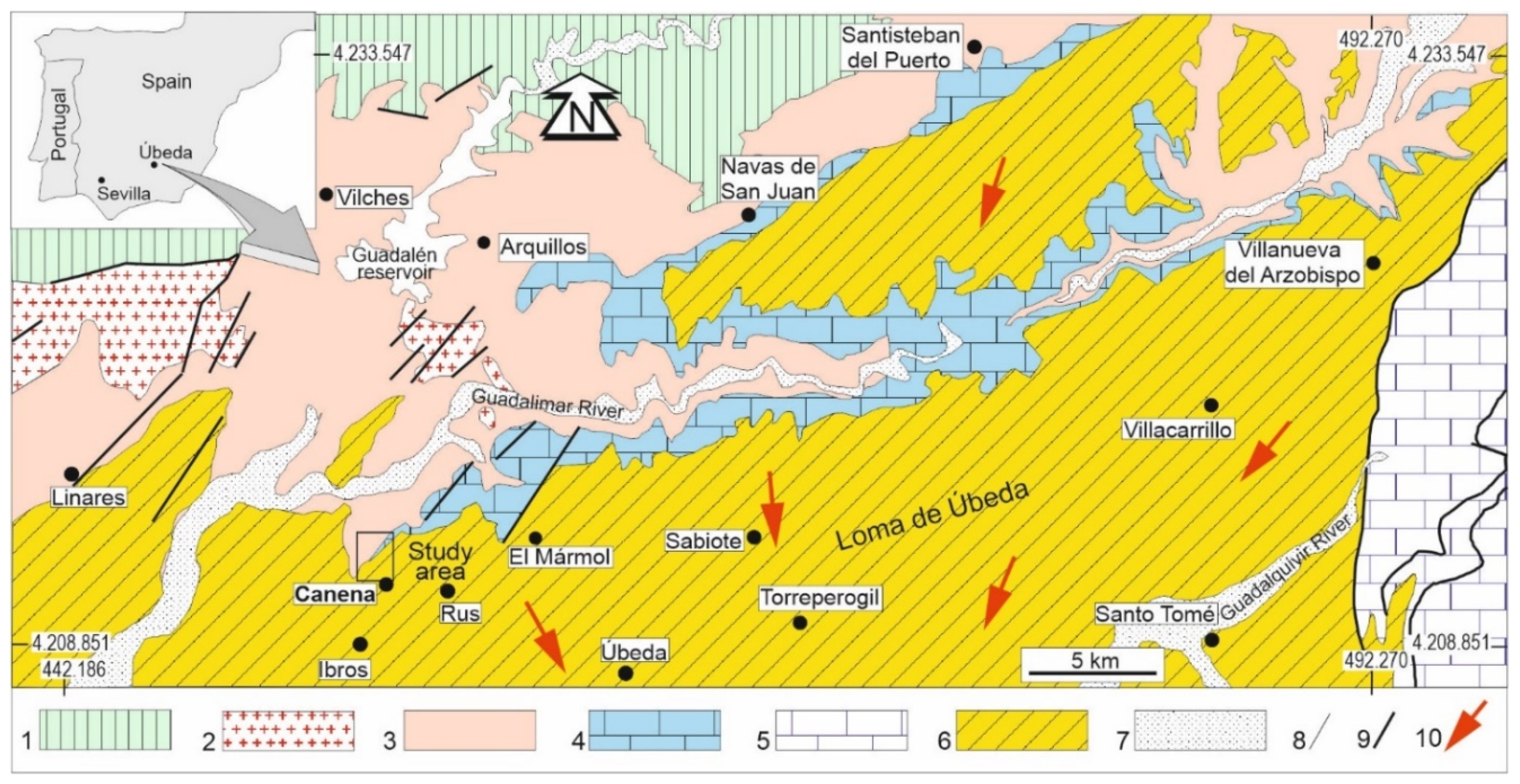
Abstract
1. Introduction
2. Description of the Study Region
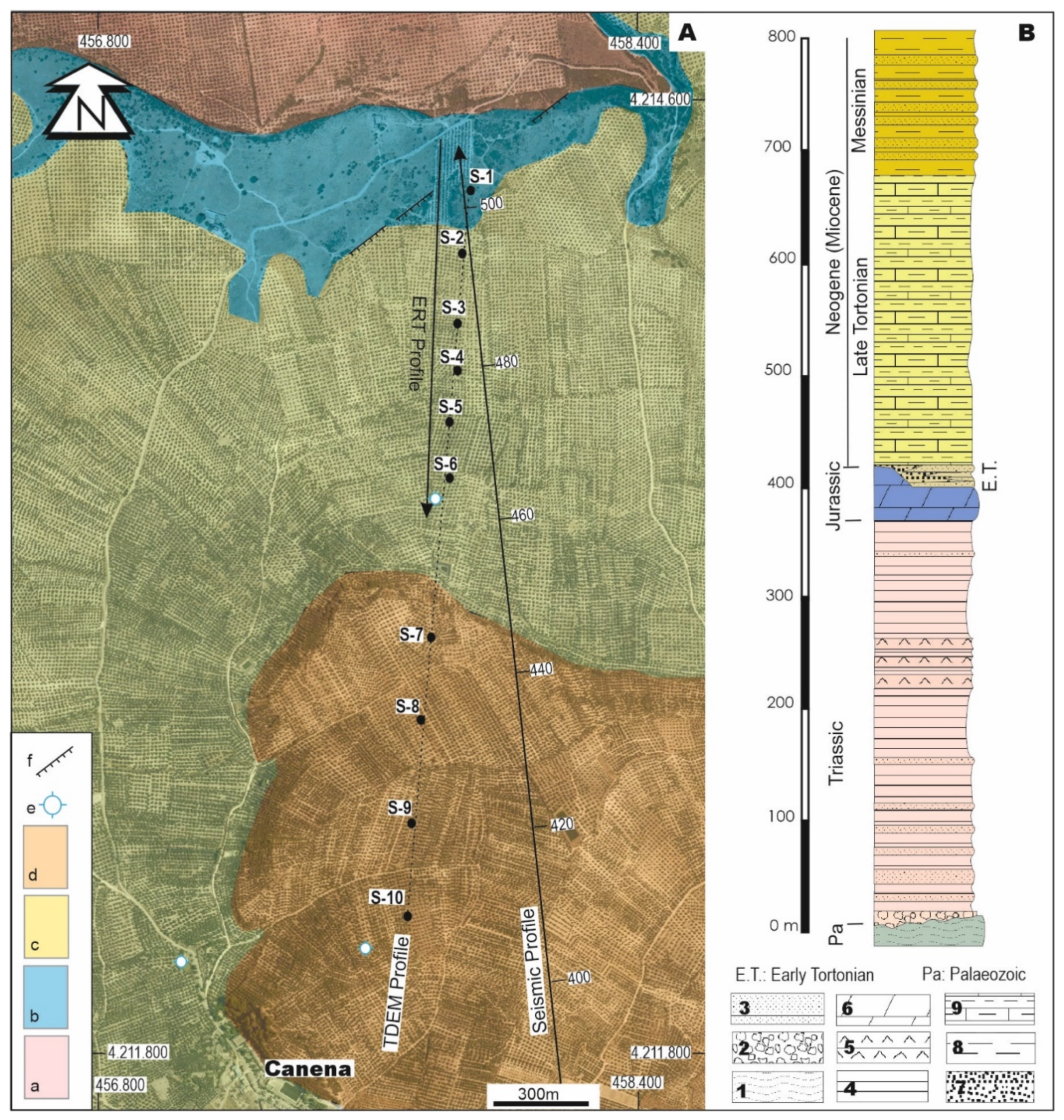
2.1. Geological Setting
2.2. Hydrogeological Context
3. Methods
3.1. Seismic Reflection
3.2. Electrical Resistivity Tomography
3.3. Time-Domain Electromagnetic
4. Results and Discussion
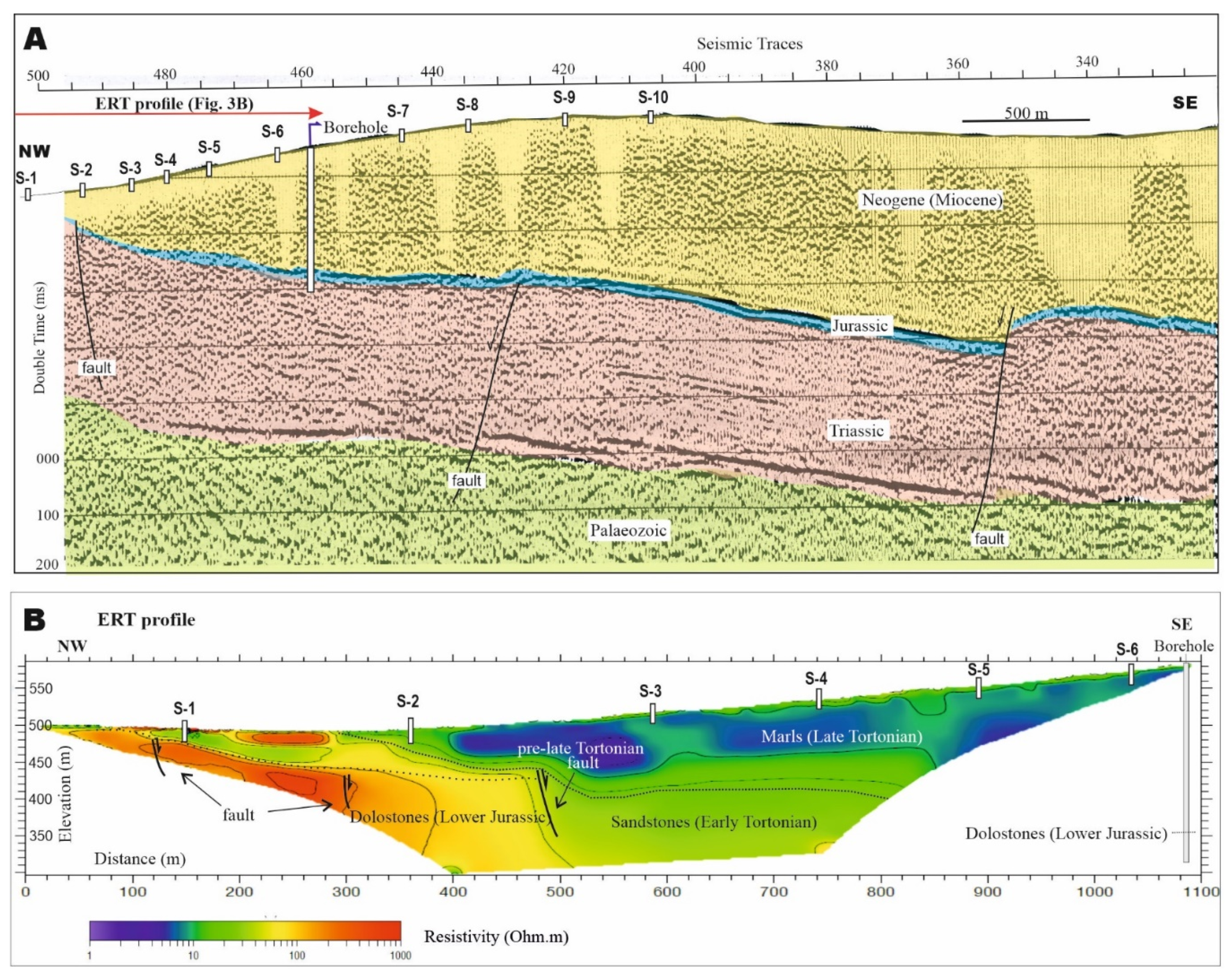
4.1. Seismic Reflection
4.2. Electrical Resistivity Tomography
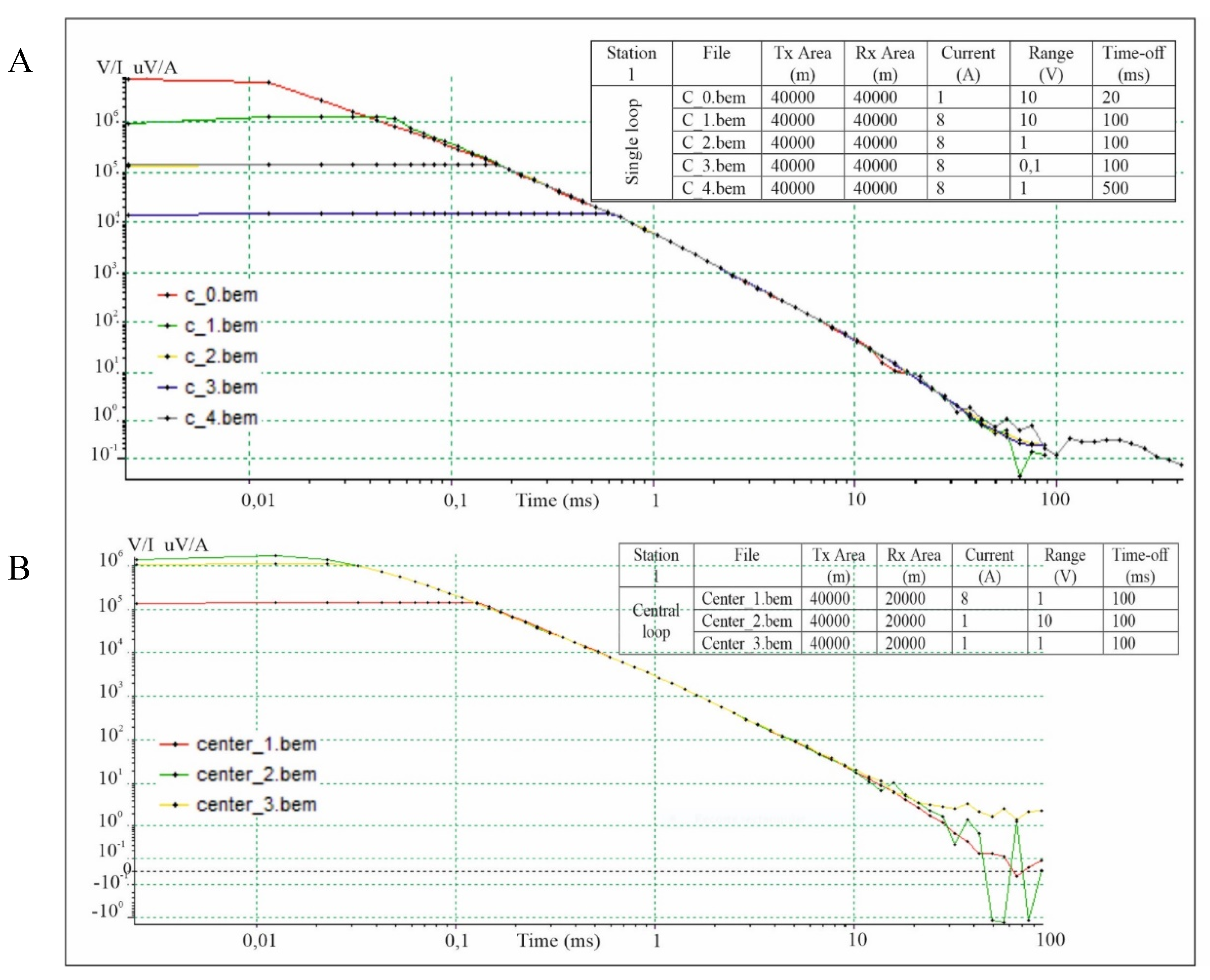
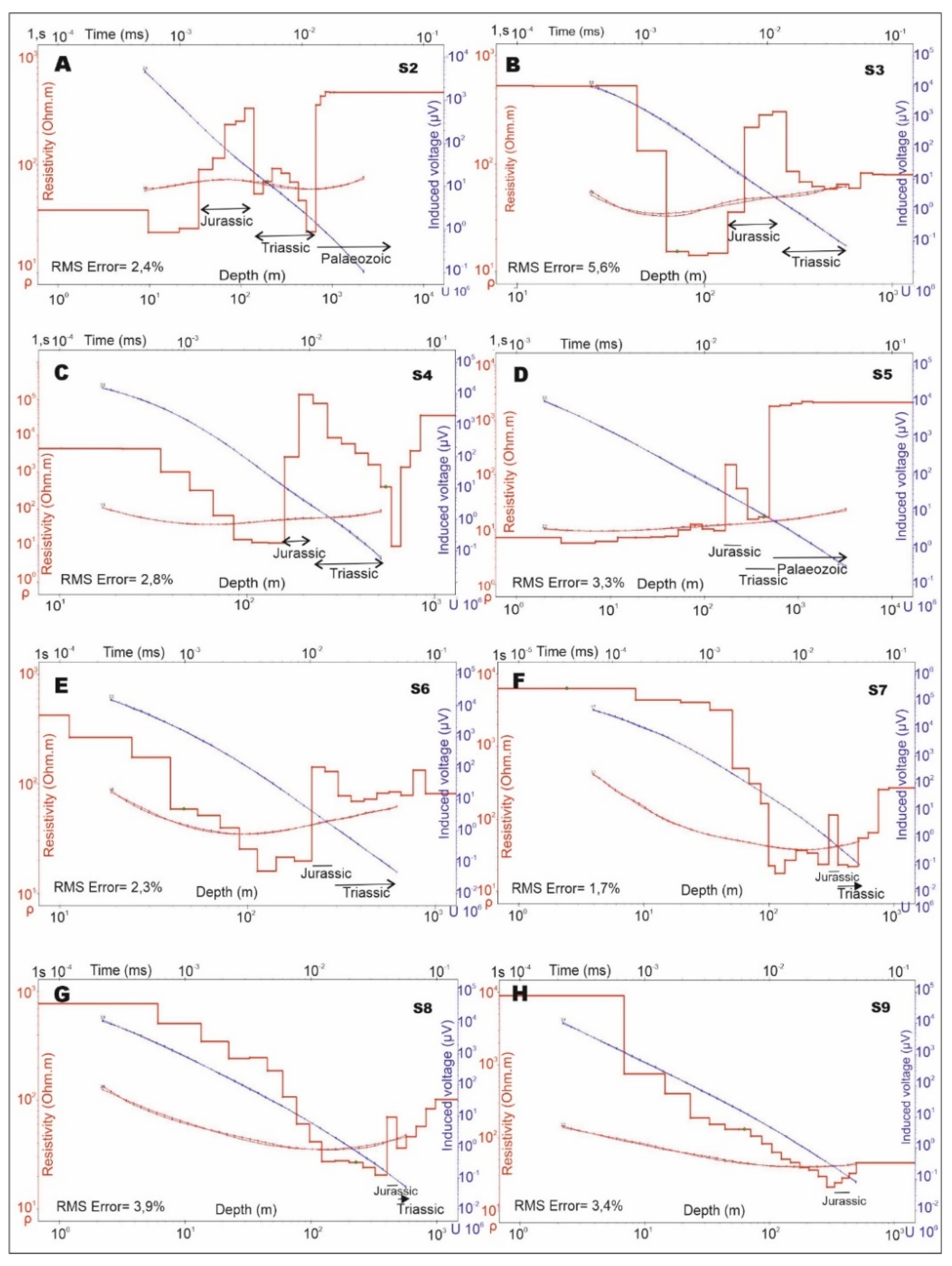
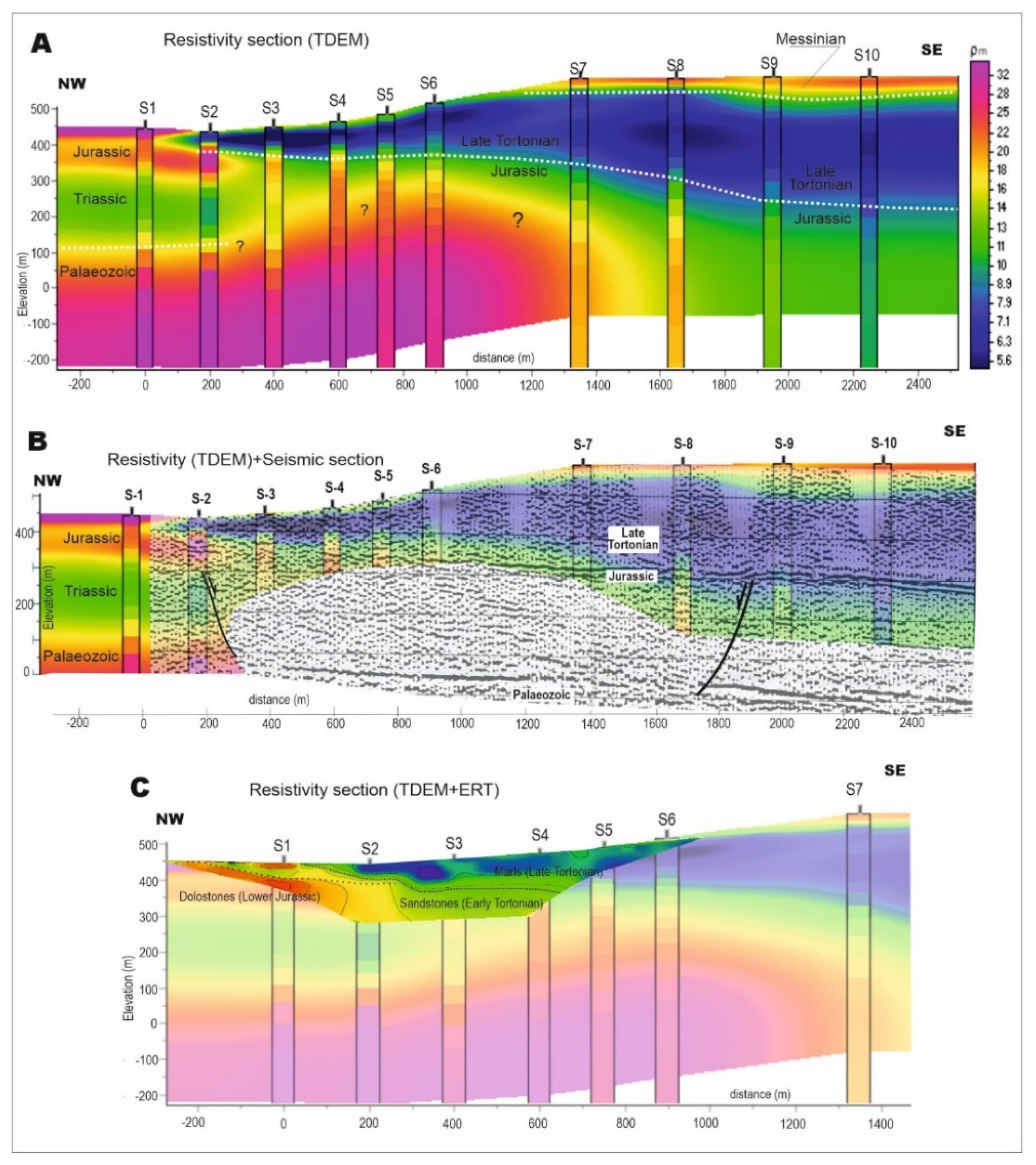
4.3. Time-Domain Electromagnetic
5. Conclusions
Author Contributions
Funding
Acknowledgments
Conflicts of Interest
References
- Griffiths, D.H.; Barker, R.D. Two-dimensional resistivity imaging and modelling in areas of complex geology. J. Appl. Geophys. 1993, 29, 211–226. [Google Scholar] [CrossRef]
- Loke, M.H.; Barker, R.D. Rapid least-squares inversion of apparent resistivity pseudosections by a quasi-Newton method. Geophys. Prospect. 1996, 44, 131–152. [Google Scholar] [CrossRef]
- André, F.; van Leeuwen, C.; Saussez, S.; Van Durmen, R.; Bogaert, P.; Moghadas, D.; de Resseguier, L.; Delvaux, B.; Vereecken, H.; Lambot, S. High-resolution imaging of a vineyard in south of France using ground-penetrating radar, electromagnetic induction and electrical resistivity tomography. J. Appl. Geophys. 2012, 78, 113–122. [Google Scholar] [CrossRef]
- Binley, A.; Hubbard, S.S.; Huisman, J.A.; Revil, A.; Robinson, D.A.; Singha, K.; Slater, L.D. The emergence of hydrogeophysics for improved understanding of subsurface processes over multiple scales. Water Resour. Res. 2015, 51, 3837–3866. [Google Scholar] [CrossRef]
- Dahlin, T.; Jens, E.; Dowen, R.; Mangeya, P.; Auken, E. Geophysical and hydrogeologic investigation of groundwater in the Karoo stratigraphic sequence at Sawmills in northern Matabeleland, Zimbabwe: A case history. Hydrogeol. J. 1999, 15, 945–960. [Google Scholar]
- Yechieli, Y.; Kafri, U.; Goldman, M.; Voss, C.I. Factor controlling of configuration of the fresh-saline water interface in the Dead Sea coastal aquifer: Synthesis of TDEM surveys and numerical groundwater modeling. Hydrogeol. J. 2001, 9, 367–377. [Google Scholar]
- Boucher, M.; Favreau, G.; Descloitres, M.; Vouillamoz, J.M.; Massuel, S.; Nazoumou, Y.; Legchenko, A. Contribution of geophysical surveys to groundwater modelling of a porous aquifer in semiarid Niger: An overview. Comptes Rendus Geosci. 2009, 341, 800–809. [Google Scholar] [CrossRef]
- Rey, J.; Redondo, L.; Hidalgo, M.C. Interés hidrogeológico de las dolomías del Liásico de la Cobertera Tabular de la Meseta (norte de Úbeda, prov. de Jaén). Rev. Soc. Geol. Esp. 1998, 11, 213–221. [Google Scholar]
- Gonzalez-Ramón, A.; Heredia, J.; Rodríguez-Arévalo, J.; Manzano, M.; Ortega, L.; Muñoz de la Varga, D.; Moreno, J.A.; Díaz Teijeiro, M.F. Evolución temporal de las características físico-químicas e isotópicas en el agua subterránea de los acuíferos de la Loma de Úbeda (sur de España). Asam. Hisp. Port. Geod. Geofís. Donostia Proc. 2012, 7, 427–434. [Google Scholar]
- I.T.G.E. Atlas Hidrogeológico de la Provincia de Jaén; ITGE-Diputación Provincial de Jaén: Jaén, España, 2012. [Google Scholar]
- Fernández, J.; Dabrio, C. Fluvial Architecture of the Buntsandstein-facies redbeds in the Middle to Upper Triassic (Ladinian-Norian) of the southeastern edge of the Iberian Meseta (Southern Spain). In Aspects of Fluvial Sedimentation in the Lower Triassic Buntsandstein of Europe; Lecture Notes in Earth Sciences; Mader, D., Ed.; Springer: Berlin, Germany, 1985; Volume 4, pp. 411–435. [Google Scholar]
- Vera, J.A.; López-Garrido, A.C. Sobre las facies detríticas rojas (red beds) del borde sureste de la Meseta. Cuad. Geol. 1971, 2, 147–155. [Google Scholar]
- Azcárate, J.E. Mapa Geológico y Memoria Explicativa de la Hoja 906 (Úbeda) del Mapa Geológico de España, Escala 1:50.000; I.G.M.E.: Madrid, Spain, 1977. [Google Scholar]
- Rey, J.; Redondo, L.; Aguado, R. Relleno, durante el Tortoniense inferior, de paleocubetas en las proximidades de Úbeda (provincia de Jaén). Bol. Geol. Min. 1995, 106, 215–218. [Google Scholar]
- Pedrera, A.; Ruiz-Constán, A.; Marín-Lechado, C.; Galindo-Zaldívar, J.; González, A.; Peláez, J.A. Seismic transpressive basement faults and monocline development in a foreland basin (Eastern Guadalquivir, SE Spain). Tectonics 2013, 32, 1571–1586. [Google Scholar] [CrossRef]
- Sánchez Gómez, M.; Peláez, J.A.; García Tortosa, F.J.; Pérez Valera, F.; Sanz de Galdeano, C. La serie sísmica de Torreperogil (Jaén, Cuenca del Guadalquivir oriental): Evidencias de deformación tectónica en el área epicentral. Rev. Soc. Geol. Esp. 2014, 27, 301–318. [Google Scholar]
- Perconing, E. Sobre la edad de la Transgresión del Terciario marino en el borde meridional de la Meseta. In Congr. Hispano-Luso-Americano de Geol. Económica; Ibérica-Tarragona: Madrid, España, 1971; Section 1; pp. 309–319. [Google Scholar]
- Hidalgo, M.C.; Rey, J.; Redondo, L. Origen de la surgencia del Balneario de San Andrés (Provincia de Jaén). Geogaceta 1998, 24, 179–182. [Google Scholar]
- González-Ramón, A.; Rodríguez-Arévalo, J.; Martos-Rosillo, S.; Gollonet, J. Hydrogeological research on intensively exploited deep aquifers in the ‘Loma de Úbeda’ area (Jaén, southern Spain). Hydrogeol. J. 2013, 21, 887–903. [Google Scholar] [CrossRef]
- Store, H.; Storz, W.; Jacobs, F. Electrical resistivity tomography to investigate geological structures of earth’s upper crust. Geophys. Prospect. 2000, 48, 455–471. [Google Scholar] [CrossRef]
- Telford, W.M.; Geldart, L.P.; Sheriff, R.E. Applied Geophysics; Cambridge University Press: Cambridge/London, UK, 1990; 770p. [Google Scholar]
- Sasaki, Y. Resolution of resistivity tomography inferred from numerical simulation. Geophys. Prospect. 1992, 40, 453–464. [Google Scholar] [CrossRef]
- Maillet, G.M.; Rizzo, E.; Revil, A.; Vella, C. High resolution electrical resistivity tomography (ERT) in a transition zone environment: Application for detailed internal architecture and infilling processes study of a Rhône River paleo-channel. Mar. Geophys. Res. 2005, 26, 317–328. [Google Scholar] [CrossRef]
- Martínez, J.; Benavente, J.; García-Aróstegui, J.L.; Hidalgo, M.C.; Rey, J. Contribution of electrical resistivity tomography to the study of detrital aquifers affected by seawater intrusión-extrusion effects: The river Vélez delta (Vélez-Málaga, southern Spain). Eng. Geol. 2009, 108, 161–168. [Google Scholar] [CrossRef]
- Rey, J.; Martínez, J.; Hidalgo, C. Investigating fluvial features with electrical resistivity imaging and ground-penetrating radar: The Guadalquivir River terrace (Jaen, Southern Spain). Sediment. Geol. 2013, 295, 27–37. [Google Scholar] [CrossRef]
- Goldman, M.; Rabinovich, B.; Rabinovich, M.; Gilad, D.; Gev, I.; Shirov, M. Application of the integrated NMR-TDEM method in groundwater exploration in Israel. J. Appl. Geophys. 1994, 31, 27–52. [Google Scholar] [CrossRef]
- Auken, E.; Jørgensen, F.; Sørensen, K.I. Large-scale TEM investigation for groundwater. Explor. Geophys. 2003, 34, 188–194. [Google Scholar] [CrossRef]
- Martínez-Pagán, P.; Faz Cano, A.; Aracil, E.; Arocena, J.M. Electrical resistivity imaging revealed the spatial properties of mine tailing ponds in the Sierra Minera of Southeast Spain. J. Environ. Eng. Geophys. 2009, 14, 63–76. [Google Scholar] [CrossRef]
- Cortada, U.; Martínez, J.; Rey, J.; Hidalgo, M.C. Assessment of tailings pond seals using geophysical and hydrochemical techniques. Eng. Geol. 2017, 223, 59–70. [Google Scholar] [CrossRef]
- Dahlin, T.; Zhou, B. A numerical comparison of 2D resistivity imaging with 10 electrode arrays. Geophys. Prospect. 2004, 52, 379–398. [Google Scholar] [CrossRef]
- Loke, M.H. Tutorial: 2-D and 3-D Electrical Imaging Surveys; Revision date: 5 November 2014. Available online: www.geotomosoft.com (accessed on 20 October 2019).
- Loke, M.H.; Dahlin, T. A comparison of the Gauss-Newton and quasi-Newton methods in resistivity imaging inversion. J. Appl. Geophys. 2002, 49, 149–162. [Google Scholar] [CrossRef]
- Nabighian, N.M. Electromagnetic Methods in Applied Geophysics-Theory; Society of Exploration Geophysics: Tulsa, OK, USA, 1988; 971p. [Google Scholar]
- Spies, B.R. Depth of investigation in electromagnetic sounding methods. Geophysics 1989, 54, 872–888. [Google Scholar] [CrossRef]
- Fitterman, D.V.; Stewart, M.T. Transient electromagnetic sounding for groundwater. Geophysics 1986, 51, 995–1005. [Google Scholar] [CrossRef]
- Gómez-Ortiz, D.; Fernández-Remolar, D.C.; Granda, A.; Quesada, C.; Granda, T.; Prieto-Ballesteros, O.; Molina, A.; Amils, R. Identification of the subsurface bodies responsible for acidity in Rio Tinto source water; Spain. Earth Planet. Sci. Lett. 2014, 391, 36–41. [Google Scholar] [CrossRef]
- Xue, G.Q.; Qin, K.Z.; Li, X.; Li, G.M.; Qi, Z.P.; Zhou, N.N. Discovery of a Large-scale Porphyry Molybdenum Deposit in Tibet through a Modified TEM Exploration Method. J. Environ. Eng. Geophys. 2012, 17, 19–25. [Google Scholar] [CrossRef]
- Granda Sanz, A.; Granda París, T.; Pons, J.M.; Videira, J.C. El descubrimiento del Yacimiento de la Magdalena. Protagonismo de los métodos geofísicos en la exploración de yacimientos tipo sulfuros masivos vulcanogénicos (vms) profundos en la faja pirítica ibérica. Bol. Geol. Min. 2019, 130, 213–230. [Google Scholar] [CrossRef]
- Danielsen, J.E.; Auken, E.; Jorgensen, F.; Sondergaard, V.; Sorensen, K. The application of the transient electromagnetic method in hydrogeophysical survey. J. Appl. Geophys. 2003, 53, 181–198. [Google Scholar] [CrossRef]
- Dennis, Z.R.; Cull, J.P. transient electromagnetic survey for the measurement of near-surface electrical anisotropy. J. Appl. Geophys. 2012, 76, 64–73. [Google Scholar] [CrossRef]
- Sridhar, M.; Markandeyulu, A.; Chaturvedi, A.K. Mapping subtrappean sediments and delineating structure with the aid of heliborne time domain electromagnetics: Case study from Kaladgi Basin, Karnataka. J. Appl. Geophys. 2017, 136, 9–18. [Google Scholar] [CrossRef]
- Hallbauer-Zadorozhnaya, V.Y.; Stettler, E. Time Domain Electromagnetic Sounding to delineare hydrocarbon Contamination of ground water. In Symposium on the Application of Geophysics to Engineering and Environmental Problems; European Association of Geoscientists & Engineers: Fort Worth, TX, USA, 2009; pp. 241–251. [Google Scholar]
- Hu, Y.; Zeng, Z.; Chen, X.; Zhao, X. Application of Transient Electromagnetic Method in saturation region detection in tailings dam. In 7th International Conference on Environmental and Engineering Geophysics & Summit Forum of Chinese Academy of Engineering on Engineering Science and Technology; Atlantis Press: Beijing, China, 2016; pp. 318–321. [Google Scholar]
- Kafri, U.; Goldman, M. Are the lower subaquifers of the Mediterranean coastal aquifer of Israel blocked to seawater intrusion? Results of a TDEM (time domain electromagnetic) study. Isr. J. Earth Sci. 2006, 55, 55–68. [Google Scholar] [CrossRef]
- Levi, E.; Goldman, M.; Hadad, A.; Gvirtzman, H. Spatial delineation of groundwater salinity using deep time domain electromagnetic geophysical measurements: A feasibility study. Water Resour. Res. 2008, 44, 1–14. [Google Scholar] [CrossRef]
- Christiansen, A.V.; Auken, E.; Sorensen, K. The transient electromagnetic method. In Groundwater Geophysics. A Tool for Hydrogeology; Kirsch, R., Ed.; Springer: Berlin, Germany, 2009; pp. 179–224. [Google Scholar]


Publisher’s Note: MDPI stays neutral with regard to jurisdictional claims in published maps and institutional affiliations. |
© 2020 by the authors. Licensee MDPI, Basel, Switzerland. This article is an open access article distributed under the terms and conditions of the Creative Commons Attribution (CC BY) license (http://creativecommons.org/licenses/by/4.0/).
Share and Cite
Rey, J.; Martínez, J.; Mendoza, R.; Sandoval, S.; Tarasov, V.; Kaminsky, A.; Hidalgo, M.C.; Morales, K. Geophysical Characterization of Aquifers in Southeast Spain Using ERT, TDEM, and Vertical Seismic Reflection. Appl. Sci. 2020, 10, 7365. https://doi.org/10.3390/app10207365
Rey J, Martínez J, Mendoza R, Sandoval S, Tarasov V, Kaminsky A, Hidalgo MC, Morales K. Geophysical Characterization of Aquifers in Southeast Spain Using ERT, TDEM, and Vertical Seismic Reflection. Applied Sciences. 2020; 10(20):7365. https://doi.org/10.3390/app10207365
Chicago/Turabian StyleRey, Javier, Julián Martínez, Rosendo Mendoza, Senén Sandoval, Vladimir Tarasov, Alex Kaminsky, M. Carmen Hidalgo, and Kevin Morales. 2020. "Geophysical Characterization of Aquifers in Southeast Spain Using ERT, TDEM, and Vertical Seismic Reflection" Applied Sciences 10, no. 20: 7365. https://doi.org/10.3390/app10207365
APA StyleRey, J., Martínez, J., Mendoza, R., Sandoval, S., Tarasov, V., Kaminsky, A., Hidalgo, M. C., & Morales, K. (2020). Geophysical Characterization of Aquifers in Southeast Spain Using ERT, TDEM, and Vertical Seismic Reflection. Applied Sciences, 10(20), 7365. https://doi.org/10.3390/app10207365