Integrated MASW and ERT Imaging for Geological Definition of an Unconfined Alluvial Aquifer Sustaining a Coastal Groundwater-Dependent Ecosystem in Southwest Portugal


 ,
, 
 , and
, and
Abstract
1. Introduction
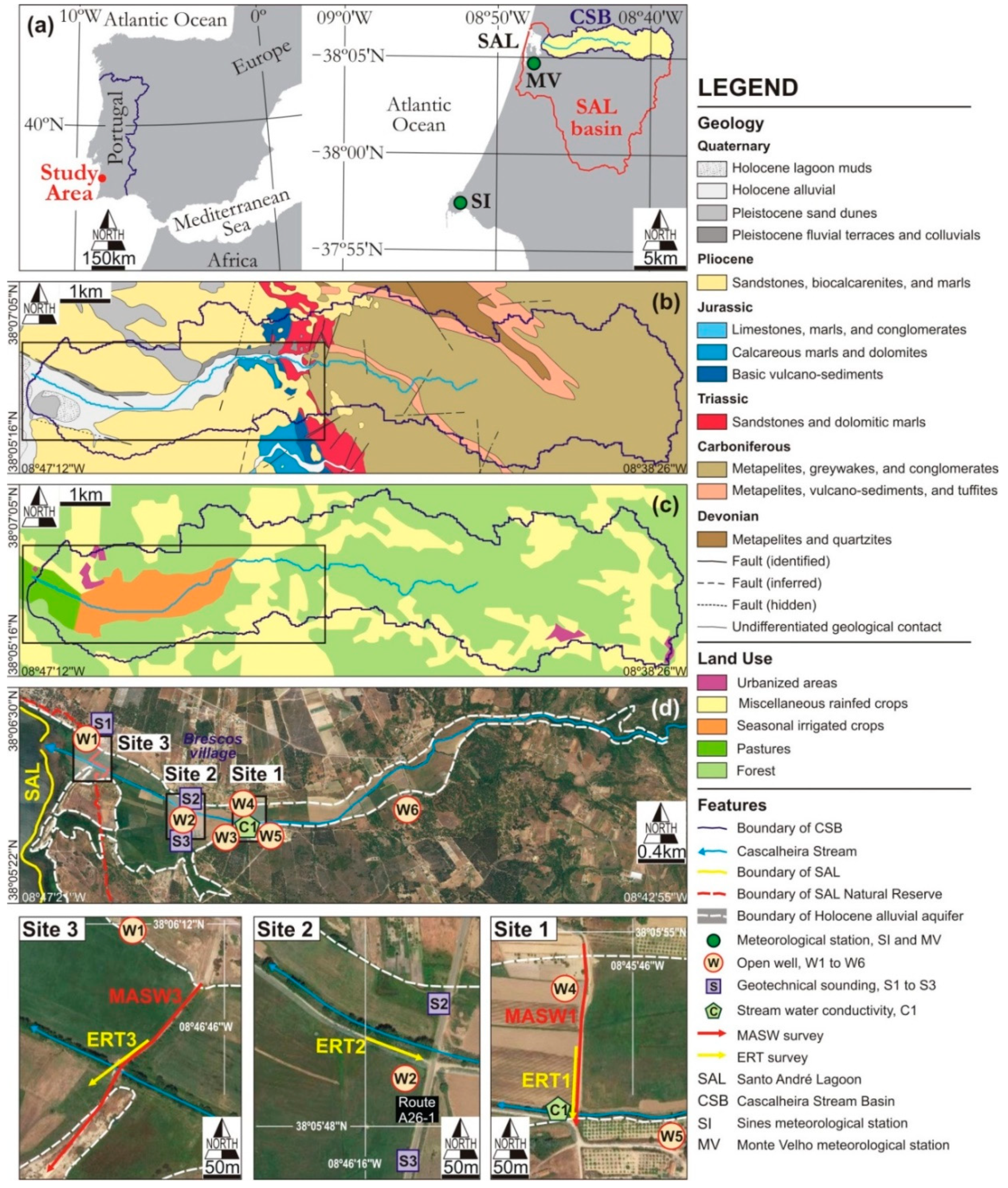
2. Study Area
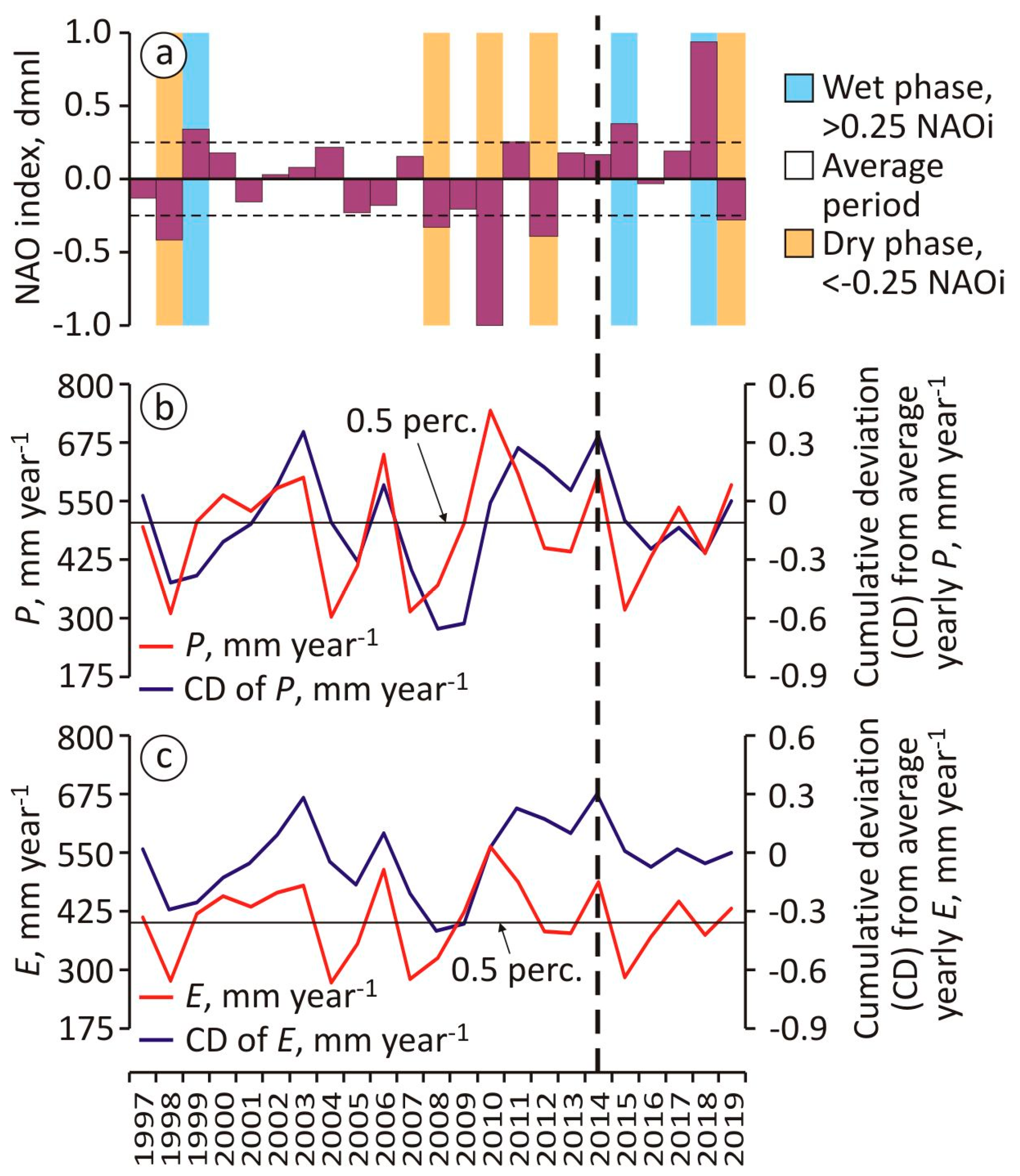
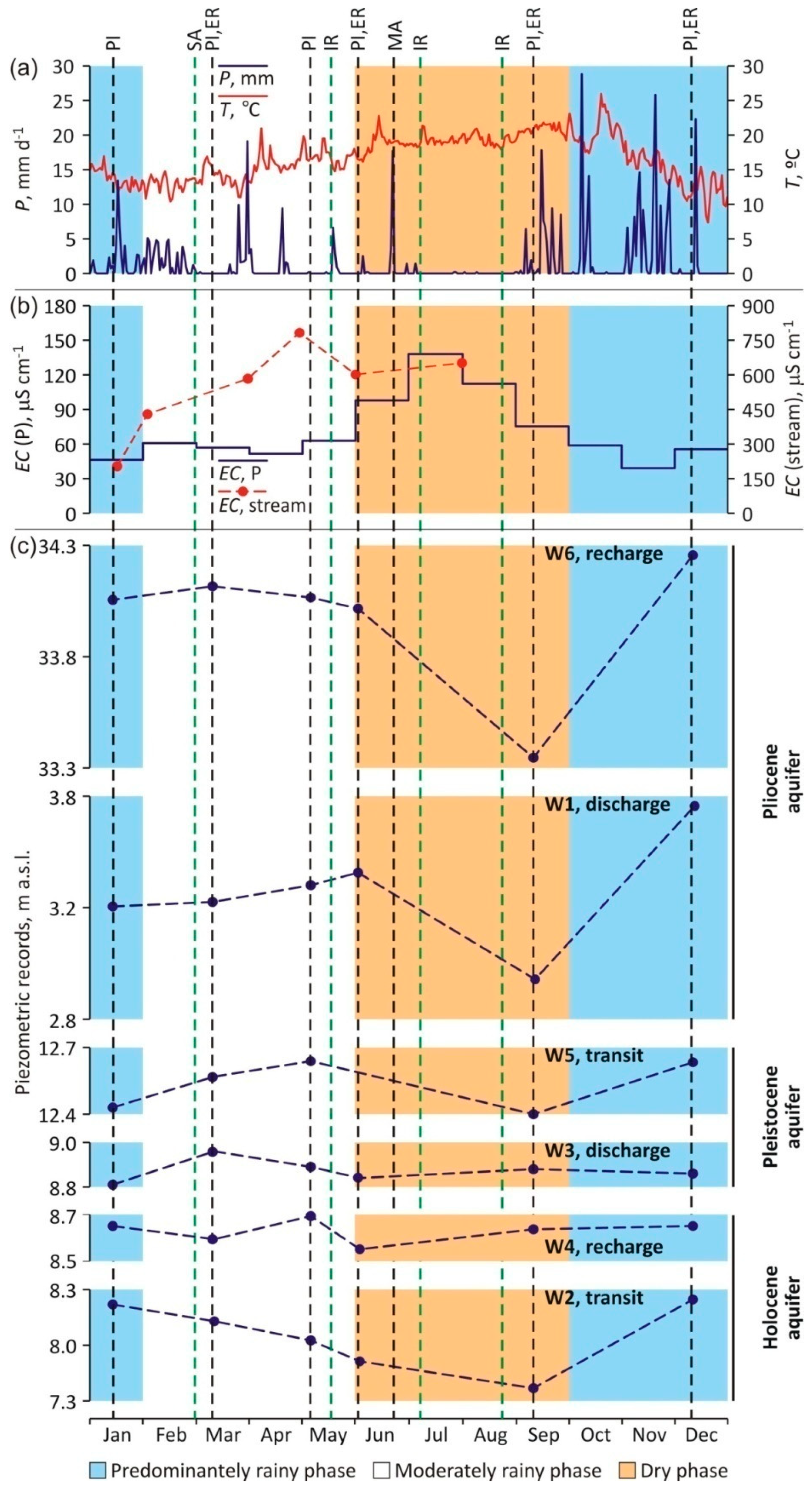
2.1. Location and Climate
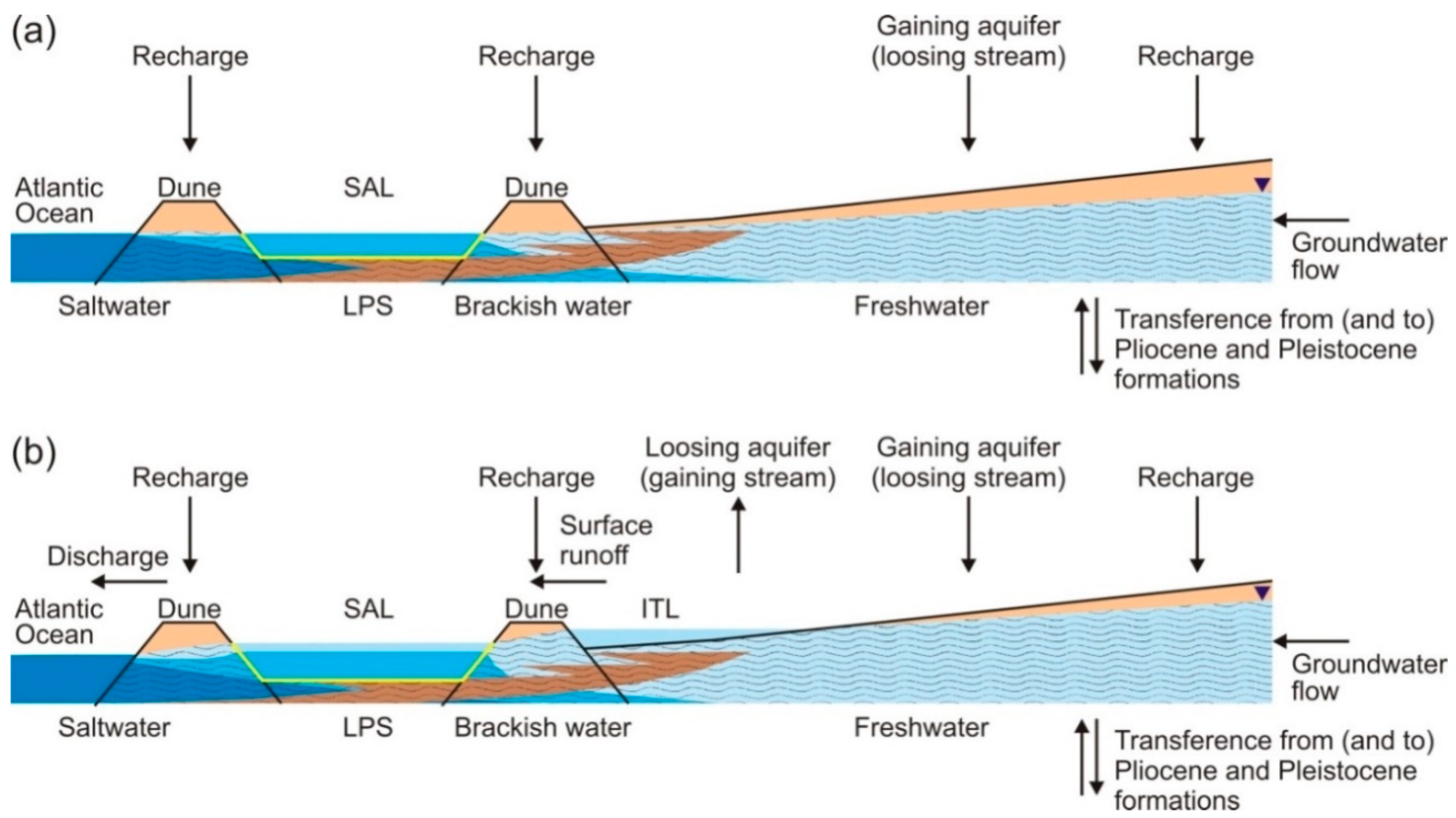
2.2. Geological and Hydrogeological Setting
2.3. Land and Groundwater Use
3. Methods
3.1. Overall Framework for Data Collection
3.2. MASW Surveys
3.3. ERT Surveys
3.4. Topographic Correction of 2D VS and ER Models
4. Results
4.1. Frequency for Geophysical Surveying
4.2. Hydrogeophysical Basis for VS and ER Models Interpretation
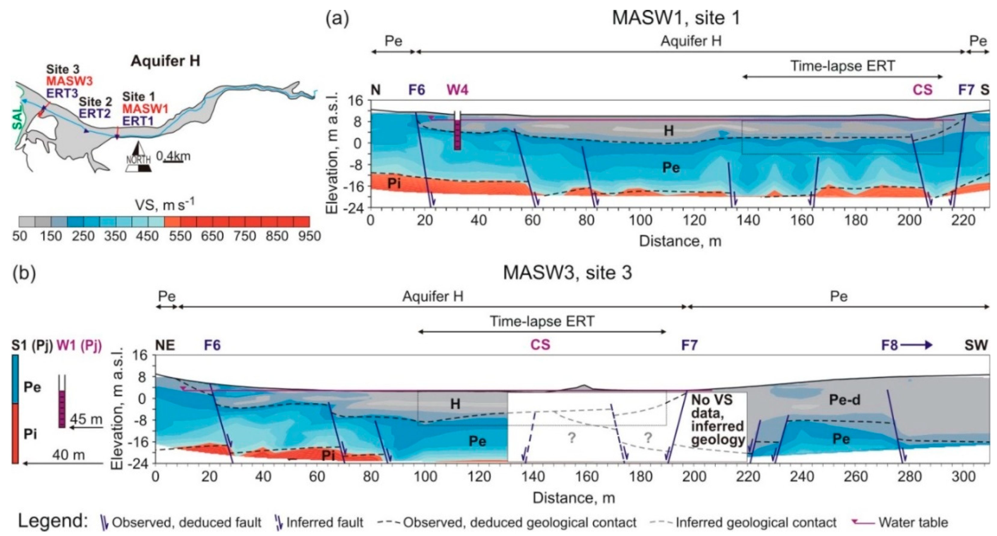
4.3. 2D VS Models
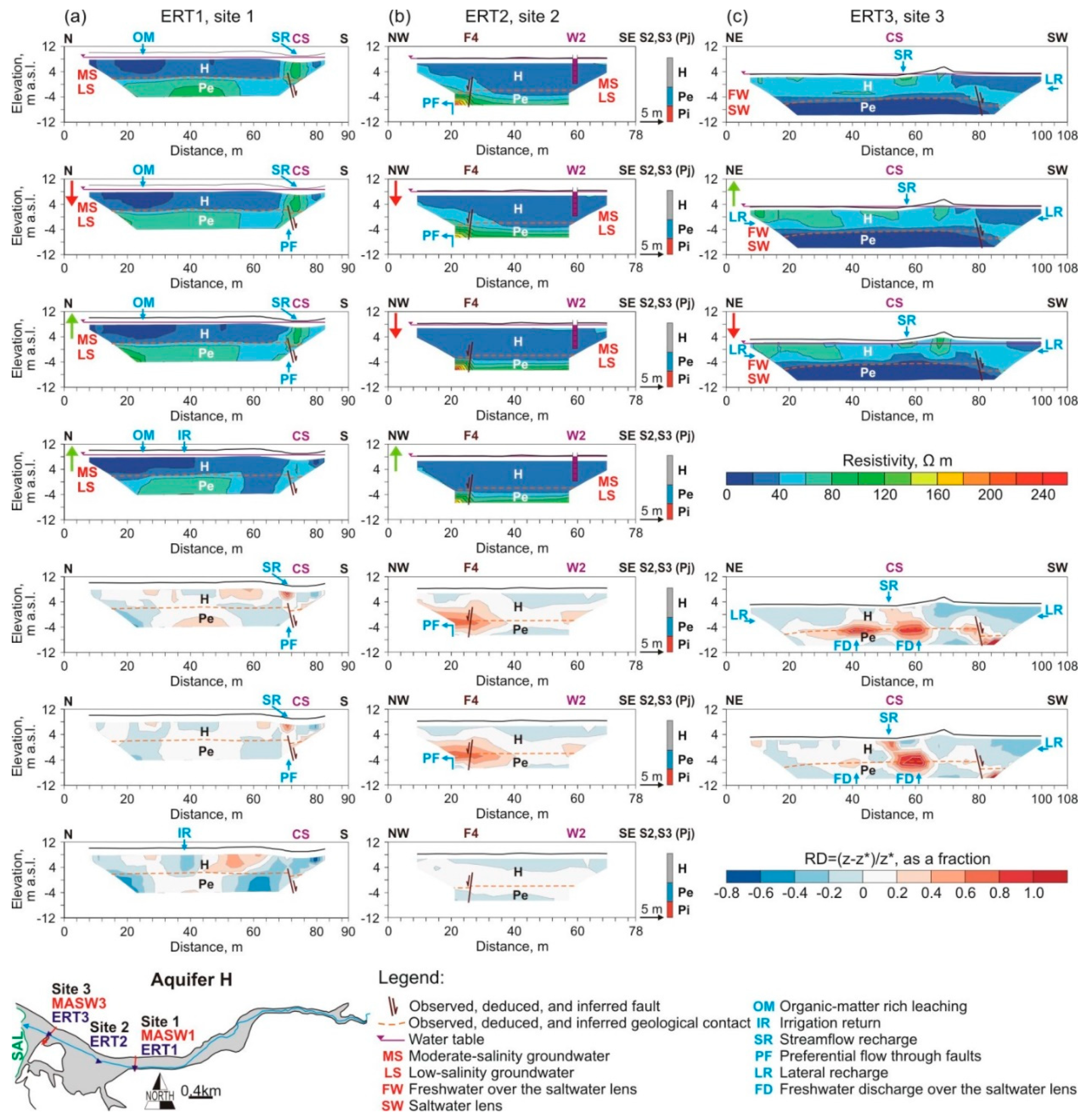
4.4. 2D ER Models
5. Discussion
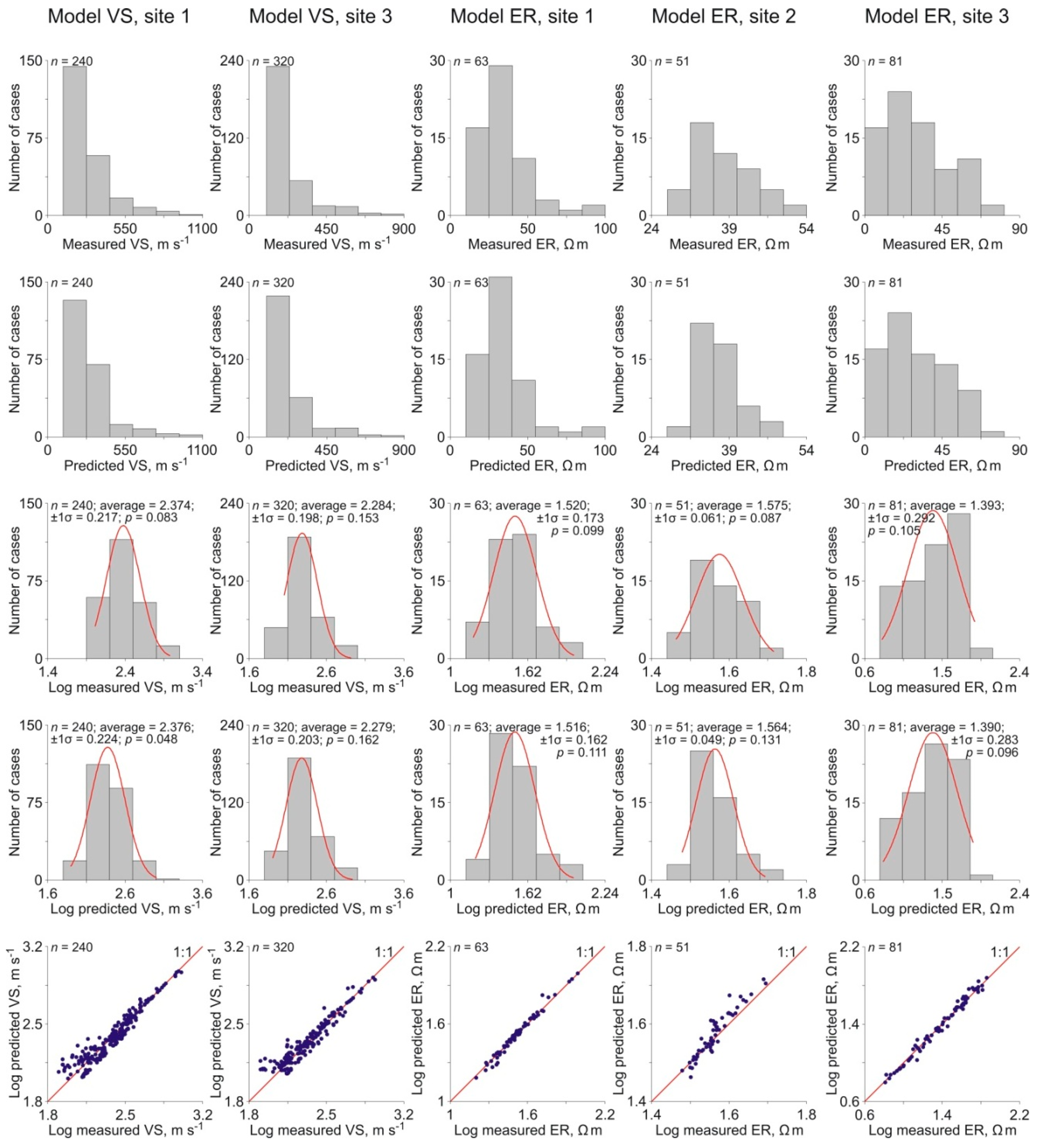
5.1. Performance of VS and ER Models
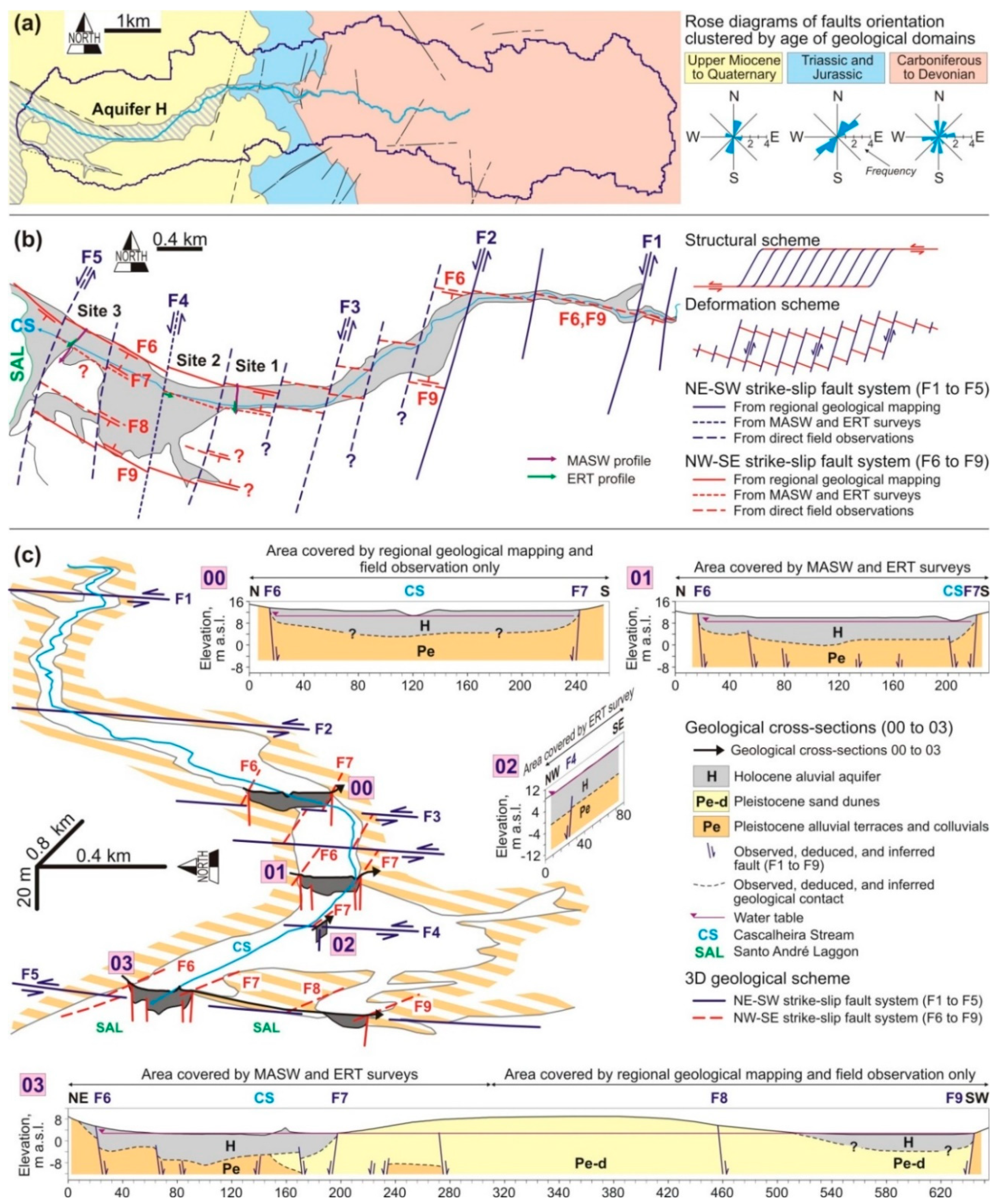
5.2. The Geological Model of the Cascalheira Stream Alluvial Aquifer
6. Conclusions
Author Contributions
Funding
Acknowledgments
Conflicts of Interest
References
- Sabater, S.; Barceló, D. Water Scarcity in the Mediterranean. Perspectives under Global Change; Springer: Berlin/Heidelberg, Germany, 2010; p. 234. [Google Scholar] [CrossRef]
- Custodio, E. Coastal aquifers of Europe: An overview. Hydrogeol. J. 2010, 18, 269–280. [Google Scholar] [CrossRef]
- Martínez-Valderrama, J.; Ibáñez, J.; Alcalá, F.J. AQUACOAST: A simulation tool to explore coastal groundwater and irrigation farming interactions. Sci. Programming-Neth 2020, 2020, 092829. [Google Scholar] [CrossRef]
- Dalin, C.; Wada, Y.; Kastner, T.; Puma, M.J. Groundwater depletion embedded in international food trade. Nature 2017, 543, 700–704. [Google Scholar] [CrossRef] [PubMed]
- Alcalá, F.J.; Martínez-Valderrama, J.; Robles-Marín, P.; Guerrera, F.; Martín-Martín, M.; Raffaelli, G.; Tejera de León, J.; Asebriy, L. A hydrological-economic model for sustainable groundwater use in sparse-data drylands: Application to the Amtoudi Oasis in southern Morocco, northern Sahara. Sci. Total Environ. 2015, 537, 309–322. [Google Scholar] [CrossRef]
- Alcalá, F.J.; Martín-Martín, M.; Guerrera, F.; Martínez-Valderrama, J.; Robles-Marín, P. A feasible methodology for groundwater resource modelling for sustainable use in sparse-data drylands: Application to the Amtoudi Oasis in the northern Sahara. Sci. Total Environ. 2018, 630, 1246–1257. [Google Scholar] [CrossRef]
- Salvador, N.; Costa, L.; Hugman, R.; Monteiro, J.P.; Stigter, T.; Nunes, L.; Duarte, D. Monitoring and modelling groundwater contributions to dependent ecosystems—The case study of the Santo André coastal lagoon. In Mudança de Planos, Proceedings of the VIII Congresso Ibérico sobre Planeamento e Gestão da Água, Lisboa, Portugal, 5–7 December 2013; Universidade Lusíada Editora: Lisboa, Portugal, 2013; Available online: http://revistas.lis.ulusiada.pt/index.php/8cigpa/article/view/386/pdf_65 (accessed on 1 May 2020).
- Paz, C.; Alcalá, F.J.; Carvalho, J.M.; Ribeiro, L. Current uses of ground penetrating radar in groundwater-dependent ecosystems research. Sci. Total Environ. 2017, 595, 868–885. [Google Scholar] [CrossRef]
- WFD. Directive 2000/60/EC of the European Parliament and of the Council of 23 October 2000 establishing a framework for Community action in the field of water policy. Off. J. Eur. Communities 2000, 327, 1–73. [Google Scholar]
- Cancela da Fonseca, L.; Chainho, P.; Félix, P.M.; Correia, M.J.; Costa, J.L.; Chaves, M.L.; Domingos, I.; Lopes, V.; Mirra, C.; Castro, J.; et al. Modelação de Cenários de Exploração em Aquíferos de Zonas Costeiras: Efeitos na Biodiversidade de Lagoas e Respectivas Ribeiras Como Ecossistemas Dependentes de água Subterrânea—Groundscene–PTDC/AAC-AMB/104639/2008–Relatório Final de Execução Científica do Projecto; Fundação para a Ciência e Tecnologia: Lisboa, Portugal, November 2013; p. 62. [Google Scholar]
- Chainho, P.; Félix, P.M.; Correia, M.J.; Fernandes, C.M.; Costa, J.L.; Chaves, M.L.; Stigter, T.; Hugman, R.; Salvador, N.; Costa, L.; et al. Projecto Groundscene: Biodiversidade de lagoas costeiras e respectivas bacias hidrográficas como ecossistemas dependentes de águas subterrâneas. In Formação e Ocupação de Litorais nas Margens do Atlântico—Brasil/Portugal; Pereira, S., Freitas, J., Bergamaschi, S., Rodrigues, M., Eds.; Fundação Carlos Chagas Filho de Amparo à Pesquisa do estado do Rio de Janeiro: Rio de Janeiro, Brazil, 2014; pp. 186–213. [Google Scholar]
- Menking, K.M.; Syed, K.H.; Anderson, R.Y.; Shafike, N.G.; Arnold, J.G. Model estimates of runoff in the closed, semiarid Estancia basin, central New Mexico, USA. Hydrol. Sci. J. 2003, 48, 953–970. [Google Scholar] [CrossRef]
- Kim, N.W.; Chung, I.M.; Won, Y.S.; Arnold, J.G. Development and application of the integrated SWAT-MODFLOW model. J. Hydrol. 2008, 356, 1–16. [Google Scholar] [CrossRef]
- Pulido-Velázquez, M.; Peña-Haro, S.; García-Prats, A.; Mocholi-Almudever, A.F.; Henriquez-Dole, L.; Macian-Sorribes, H.; Lopez-Nicolas, A. Integrated assessment of the impact of climate and land use changes on groundwater quantity and quality in the Mancha Oriental system (Spain). Hydrol. Earth Syst. Sci. 2015, 19, 1677–1693. [Google Scholar] [CrossRef]
- Poeter, E.; Anderson, D. Multimodel ranking and inference in ground water modeling. Groundwater 2005, 43, 597–605. [Google Scholar] [CrossRef] [PubMed]
- Hojberg, A.L.; Refsgaard, J.C. Model uncertainty-parameter uncertainty versus conceptual models. Water Sci. Technol. 2005, 52, 177–186. [Google Scholar] [CrossRef] [PubMed]
- Beven, K. Towards integrated environmental models of everywhere: Uncertainty, data and modelling as a learning process. Hydrol. Earth Syst. Sci. 2007, 11, 460–467. [Google Scholar] [CrossRef]
- Monteiro Santos, F.A.; Sultan, S.A.; Represas, P.; El Sorady, A.L. Joint inversion of gravity and geoelectric data for groundwater and structural investigation: Application to the northwestern part of Sinai, Egypt. Geophys. J. Int. 2006, 165, 705–718. [Google Scholar] [CrossRef]
- Khalil, M.A.; Hafez, M.A.; Santos, F.M.; Ramalho, E.C.; Mesbah, H.S.; El-Qady, G.M. An approach to estimate porosity and groundwater salinity by combined application of GPR and VES: A case study in the Nubian sandstone aquifer. Near Surf. Geophys. 2010, 8, 223–233. [Google Scholar] [CrossRef]
- Alam, K.; Ahmad, N. Determination of aquifer geometry through geophysical methods: A case study from Quetta Valley, Pakistan. Acta Geophys. 2014, 62, 142–163. [Google Scholar] [CrossRef]
- Farzamian, M.; Monteiro Santos, F.A.; Khalil, M.A. Estimation of unsaturated hydraulic parameters in sandstone using electrical resistivity tomography under a water injection test. J. Appl. Geophys. 2015, 121, 71–83. [Google Scholar] [CrossRef]
- Binley, A.; Hubbard, S.S.; Huisman, J.A.; Revil, A.; Robinson, D.A.; Singha, K.; Slater, L.D. The emergence of hydrogeophysics for improved understanding of subsurface processes over multiple scales. Water Resour. Res. 2015, 51, 3837–3866. [Google Scholar] [CrossRef]
- Uhlemann, S.S.; Sorensen, J.P.R.; House, A.R.; Wilkinson, P.B.; Roberts, C.; Gooddy, D.C.; Binley, A.M.; Chambers, J.E. Integrated time-lapse geoelectrical imaging of wetland Hydrol Process. Water Resour. Res. 2016, 52, 3. [Google Scholar] [CrossRef]
- Gonçalves, R.; Farzamian, M.; Monteiro Santos, F.A.; Represas, P.; Mota Gomes, A.; Lobo de Pina, A.F.; Almeida, E.P. Application of Time-Domain Electromagnetic Method in Investigating Saltwater Intrusion of Santiago Island (Cape Verde). Pure Appl. Geophys. 2017, 174, 4171–4182. [Google Scholar] [CrossRef]
- Xia, J.; Miller, R.D.; Park, C.B. Estimation of near-surface shear-wave velocity by inversion of Rayleigh wave. Geophysics 1999, 64, 691–700. [Google Scholar] [CrossRef]
- Xia, J.; Miller, R.D.; Park, C.B.; Hunter, J.A.; Harris, J.B.; Ivanov, J. Comparing shear-wave velocity profiles inverted from multichannel surface wave with borehole measurements. Soil Dyn. Earthq. Eng. 2002, 22, 181–190. [Google Scholar] [CrossRef]
- Park, C.B.; Miller, R.D.; Xia, J. Multi-channel analysis of surface waves. Geophysics 1999, 64, 800–808. [Google Scholar] [CrossRef]
- Park, C.B.; Miller, R.D.; Xia, J.; Ivanov, J. Multichannel analysis of surface waves (MASW)—Active and passive methods. Lead Edge 2007, 26, 60–64. [Google Scholar] [CrossRef]
- Hayley, K.; Bentley, L.R.; Gharibi, M.; Nightingale, M. Low temperature dependence of electrical resistivity: Implications for near surface geophysical monitoring. Geophys. Res. Lett. 2007, 34, L18402. [Google Scholar] [CrossRef]
- Hayley, K.; Bentley, L.R.; Gharibi, M. Time-lapse electrical resistivity monitoring of salt-affected soil and groundwater. Water Resour. Res. 2010, 45, W07425. [Google Scholar] [CrossRef]
- Steelman, C.M.; Kennedy, C.S.; Capes, D.C.; Parker, B.L. Electrical resistivity dynamics beneath a fractured sedimentary bedrock riverbed in response to temperature and groundwater–surface water exchange. Hydrol. Earth Syst. Sci. 2017, 21, 3105–3123. [Google Scholar] [CrossRef]
- Giustiniani, M.; Accaino, F.; Picotti, S.; Tinivella, U. Characterization of the shallow aquifers by high-resolution seismic data. Geophys. Prospect. 2008, 56, 655–666. [Google Scholar] [CrossRef]
- Martorana, R.; Lombardo, L.; Messina, N.; Luzio, D. Integrated geophysical survey for 3D modelling of a coastal aquifer polluted by seawater. Near Surf. Geophys 2014, 12, 45–59. [Google Scholar] [CrossRef]
- Foti, S.; Hollender, F.; Garofalo, F.; Albarello, D.; Asten, M.; Bard, P.-Y.; Comina, C.; Cornou, C.; Cox, B.; Giulio, G.D.; et al. Guidelines for the good practice of surface wave analysis: A product of the InterPACIFIC project. Bull. Earthq. Eng. 2018, 16, 2367–2420. [Google Scholar] [CrossRef]
- Benjumea, B.; Gabàs, A.; Macau, A.; Bellmunt, F.; Figueras, S.; Vilà, M.; Pi, R. Combination of Geophysical Techniques to Characterize Sediments (Ebro Delta, Spain). In Proceedings of the Near Surface Geoscience 2016—22nd European Meeting of Environmental and Engineering Geophysics, Barcelona, Spain, 4–6 September 2016; European Association of Geoscientists & Engineers: Houten, The Netherlands, 2016. [Google Scholar] [CrossRef]
- Billy, J.; Baudouin, V.; Portal, A.; Deparis, J.; Bitri, A.; Garcin, M. An Innovative Approach for a Comprehensive Characterization of Coastal Dune Systems through Internal Architecture and the Associated Intrinsic Geophysical Properties. J. Coast. Res. 2020, 95, 387–391. [Google Scholar] [CrossRef]
- Glazer, M.; Dobiński, W.; Marciniak, A.; Majdański, M.; Błaszczyk, M. Spatial distribution and controls of permafrost development in non-glacial Arctic catchment over the Holocene, Fuglebekken, SW Spitsbergen. Geomorphology (Amst) 2020, 358, 107128. [Google Scholar] [CrossRef]
- Telford, W.M.; Geldart, L.P.; Sheriff, R.E. Applied Geophysics, 2nd ed.; Cambridge University Press: New York, NY, USA, 1990. [Google Scholar]
- Alcalá, F.J.; Custodio, E. Atmospheric chloride deposition in continental Spain. Hydrol. Process. 2008, 22, 3636–3650. [Google Scholar] [CrossRef]
- Ramos, R. Contribuição dos Métodos Geofísicos Para o Modelo Evolutivo da Região de Santo André Desde o último Máximo Glaciário. Ph.D. Thesis, University of Lisbon, Lisbon, Portugal, 2013. Available online: http://hdl.handle.net/10451/10795 (accessed on 1 May 2020).
- Trigo, R.M.; Pozo-Vázquez, D.; Osborn, T.J.; Castro-Díez, Y.; Gámiz-Fortis, S.; Esteban-Parra, M.J. North Atlantic Oscillation influence on precipitation, river flowand water resources in the Iberian Peninsula. Int. J. Climatol. 2004, 24, 925–944. [Google Scholar] [CrossRef]
- APA. Plano de Gestão das Bacias Hidrográficas Integradas nas Regiões Hidrográficas 6 e 7; Agência Portuguesa do Ambiente: Lisboa, Portugal, 2012; Volume 1.
- LNEG. Geological Map of Portugal, Scale 1:50,000; Sheet nº 42-A, Grândola; National Laboratory of Energy and Geology of Portugal, Memory and Maps. 2011. Available online: http://geoportal.lneg.pt/geoportal/egeo/DownloadCartas/ (accessed on 28 February 2020).
- Dias, R.; Araújo, A.; Terrinha, P.; Kullberg, J.C. (Eds.) Geologia de Portugal; Escolar Editora: Lisboa, Portugal, 2013; Volume 2, p. 1624. [Google Scholar]
- Quesada, C.; Oliveira, J.T. (Eds.) The Geology of Iberia: A Geodynamic Approach; Springer Nature Switzerland AG: Cham, Switzerland, 2020. [Google Scholar] [CrossRef]
- Almeida, C.; Mendonça, J.J.; Jesus, M.R.; Gomes, J. Sistemas Aquíferos de Portugal Continental; Centro de Geologia da FCUL, Instituto da Água: Lisboa, Portugal, 2000; p. 649. [Google Scholar]
- Freitas, M.C.; Andrade, C.; Rocha, F.; Tassinari, C.; Munhá, J.M.; Cruces, A.; Vidinha, J.; Silva, C.M. Late glacial and Holocene environmental changes in Portuguese coastal lagoons 1: The sedimentological and geochemical records of the Santo André coastal area. Holocene 2003, 13, 433–446. [Google Scholar] [CrossRef]
- Cearreta, A.; Cachão, M.; Cabral, M.C.; Bao, R.; Ramalho, M.J. Lateglacial and Holocene environmental changes in Portuguese coastal lagoons 2: Microfossil multiproxy reconstruction of the Santo André coastal area. Holocene 2003, 13, 447–458. [Google Scholar] [CrossRef]
- Pires, A.R.M. Morfodinâmica da Barra de Maré Efémera da Lagoa de Santo André. Master’s Thesis, University of Lisbon, Lisbon, Portugal, 2011. Available online: http://hdl.handle.net/10451/8451 (accessed on 1 May 2020).
- Lobo-Ferreira, J.P.C.; Oliveira, M.M.; Moinante, M.J.; Leitão, T.E.; Novo, M.E.; Moreira, P.E.; Henriques, M.J. Caracterização dos Recursos Hídricos Subterrâneos da Área Abrangida pelo Plano de Bacia Hidrográfica do Rio Sado.Anexo 4 Recursos Hídricos Subterrâneos. Relatório Provisório da Fase I; Laboratório Nacional de Engenharia Civil: Lisboa, Portugal, October 1999; p. 135.
- Monteiro, J.P.; Chambel, A.; Martins, J. Conceptual and Numerical Flow Model of the Sines Aquifer System (Alentejo, South Portugal). International Groundwater Symposium; International Association of Hydraulic Engineering and Research (IAHR): Istanbul, Turkey, 2008; p. 38 (abstract) and p. 9 (CD-Rom). [Google Scholar]
- Alcalá, F.J.; Cantón, Y.; Contreras, S.; Were, A.; Serrano-Ortiz, P.; Puigdefábregas, J.; Solé-Benet, A.; Custodio, E.; Domingo, F. Diffuse and concentrated recharge evaluation using physical and tracer techniques: Results from a semiarid carbonate massif aquifer in southeastern Spain. Environ. Earth Sci. 2011, 63, 541–557. [Google Scholar] [CrossRef]
- Kim, J.; Supper, R.; Tsourlos, P.; Yi, M. Four-dimensional inversion of resistivity monitoring data through Lp norm minimizations. Geophys. J. Int. 2013, 195, 1640–1656. [Google Scholar] [CrossRef]
- Loke, M.H. Rapid 2-D Resistivity & IP Inversion Using the Least-squares Method; Geotomo Software: Penang, Malaysia, 2012. [Google Scholar]
- Chapman, T.G. A comparison of algorithms for stream flow recession and baseflow separation. Hydrol. Process 1999, 13, 701–714. [Google Scholar] [CrossRef]
- IPCC. Climate Change 2007: Impacts, Adaptation and Vulnerability. Contribution of Working Group II to the Fourth Assessment Report of the Intergovernmental Panel on Climate Change; Cambridge University Press: Cambridge, UK, 2007. [Google Scholar]
- Navarro, M.; Vidal, F.; Enomoto, T.; Alcalá, F.; García-Jerez, A.; Sánchez, F.J.; Abeki, N. Analysis of the weightiness of site effects on reinforced concrete (RC) building seismic behavior. The Adra town example (SE Spain). Earthq. Eng. Struct. D 2007, 36, 1363–1383. [Google Scholar] [CrossRef]
- García-Jerez, A.; Navarro, M.; Alcalá, F.J.; Luzón, F.; Pérez-Ruiz, J.A.; Enomoto, T.; Vidal, F.; Ocaña, E. Shallow velocity structure using joint inversion of array and h/v spectral ratio of ambient noise: The case of Mula town (SE of Spain). Soil Dyn. Earthq. Eng. 2007, 27, 907–919. [Google Scholar] [CrossRef]
- Martínez-Pagán, P.; Navarro, M.; Pérez-Cuevas, J.; Alcalá, F.J.; García-Jerez, A.; Vidal, F. Shear-wave velocity structure from MASW and SPAC methods. The case of Adra town, SE Spain. Near Surf. Geophys. 2018, 16, 356–371. [Google Scholar] [CrossRef]
- Alcalá, F.J.; Espinosa, J.; Navarro, M.; Sánchez, F.J. Propuesta de división geológica de la localidad de Adra (provincia de Almería). Aplicación a la zonación sísmica. Rev. Soc. Geológica España 2002, 15, 55–66. [Google Scholar]
- Mitchell, J.K.; Soga, K. Fundamentals of Soil Behaviour; Wiley: London, UK, 2005. [Google Scholar]
- Zimmer, M.A.; Prasad, M.; Mavko, G.; Nur, A. Seismic velocities of unconsolidated sands: Part 1—Pressure trends from 0.1 to 20 MPa. Geophysics 2007, 72, E1–E13. [Google Scholar] [CrossRef]
- Martínez-Pagán, P.; Navarro, M.; Pérez-Cuevas, J.; Alcalá, F.J.; García-Jerez, A.; Sandoval-Castaño, S. Shear-wave velocity based seismic microzonation of Lorca city (SE Spain) from MASW analysis. Near Surf. Geophys. 2014, 12, 739–749. [Google Scholar] [CrossRef]
- McGann, C.R.; Bradley, B.A.; Cubrinovski, M. Investigation of shear wave velocity depth variability, site classification, and liquefaction vulnerability identification using a near-surface Vs model of Christchurch, New Zealand. Soil Dyn. Earthq. Eng. 2017, 92, 692–705. [Google Scholar] [CrossRef]
- Alcalá, F.J.; Custodio, E. Natural uncertainty of spatial average aquifer recharge through atmospheric chloride mass balance in continental Spain. J. Hydrol. 2015, 524, 642–661. [Google Scholar] [CrossRef]
- Willmott, C.J.; Matsuura, K. Advantages of the mean absolute error (MAE) over the root mean square error (RMSE) in assessing average model performance. Clim. Res. 2005, 30, 79–82. [Google Scholar] [CrossRef]
- Chai, T.; Draxler, R.R. Root mean square error (RMSE) or mean absolute error (MAE)?—Arguments against avoiding RMSE in the literature. Geosci. Model. Dev. 2014, 7, 1247–1250. [Google Scholar] [CrossRef]
- Hyndman, R.J.; Koehler, A.B. Another look at measures of forecast accuracy. Int. J. Forecast. 2006, 22, 679–688. [Google Scholar] [CrossRef]
- Moriasi, D.N.; Wilson, B.N.; Douglas-Mankin, K.R.; Arnold, J.G.; Gowda, P.H. Hydrologic and water quality models: Use, calibration, and validation. Trans. ASABE 2012, 55, 1241–1247. [Google Scholar] [CrossRef]
- Lin, L.; Hedayat, A.S.; Wu, W. Statistical Tools for Measuring Agreement; Springer: New York, NY, USA, 2012. [Google Scholar]
- Frid, V.; Averbach, A.; Frid, M.; Dudkinski, D.; Liskevich, G. Statistical Analysis of Resistivity Anomalies Caused by Underground Caves. Pure Appl. Geophys. 2017, 174, 997–1012. [Google Scholar] [CrossRef]
- Frid, V.; Sharabi, I.; Frid, M.; Averbakh, A. Leachate detection via statistical analysis of electrical resistivity and induced polarization data at a waste disposal site (Northern Israel). Environ. Earth Sci. 2017, 76, 233. [Google Scholar] [CrossRef]
- Vásconez-Maza, M.D.; Martínez-Segura, M.A.; Bueso, M.C.; Faz, A.; García-Nieto, M.C.; Gabarrón, M.; Acosta, J.A. Predicting spatial distribution of heavy metals in an abandoned phosphogypsum pond combining geochemistry, electrical resistivity tomography and statistical methods. J. Hazard. Mater. 2019, 374, 392–400. [Google Scholar] [CrossRef] [PubMed]


| Acronym | Definition |
|---|---|
| Aquifer H | Holocene alluvial aquifer |
| CSB | Cascalheira Stream Basin |
| CVMAE | Normalized MAE |
| CVRMSE | Normalized RMSE |
| CVSTD | Normalized STD |
| EC | Electrical conductivity |
| ER | Electrical resistivity |
| ERT | Electrical resistivity tomography |
| GDE | Groundwater-dependent ecosystem |
| GEC | Groundwater electrical conductivity |
| GER | Groundwater electrical resistivity |
| lnNSE | Logarithmic form of NSE |
| MAE | Mean error |
| MASW | Multichannel analysis of surface waves |
| MRE | Mean relative error |
| NAO | North Atlantic Oscillation |
| NSE | Nash–Sutcliffe efficiency coefficient |
| PBIAS | Percent bias |
| R2 | Coefficient of determination |
| RD | Relative difference |
| RMSE | Root-mean-square error |
| RSR | RMSE relative to STD |
| SAL | Santo André Lagoon |
| STD | Standard deviation of the measured data |
| SWQM | SAL water quality monitoring |
| VS | Shear-wave velocity |
| WFD | European Water Framework Directive |
| Site | Profile ID 1 | Length, m | Prospecting Depth, m | Date |
|---|---|---|---|---|
| 1 | MASW1 | 230 | 30 | 23 June 2014 |
| ERT1 | 90 | 13 | 13 March 2014 | |
| 4 June 2014 | ||||
| 12 September 2014 | ||||
| 10 December 2014 | ||||
| 2 | ERT2 | 78 | 15 | 13 March 2014 |
| 4 June 2014 | ||||
| 12 September 2014 | ||||
| 10 December 2014 | ||||
| 3 | MASW3 | 310 | 27 | 23 June 2014 |
| ERT3 | 108 | 13 | 12 March 2014 | |
| 3 June 2014 | ||||
| 10 September 2014 |
| Site | ID 1 | Elevation, m a.s.l. | Aquifer and Flow Zone | Variable 2 | GEC 3 | GER 4 |
|---|---|---|---|---|---|---|
| Upstream | W6 | 35.18 | Pliocene, recharge | PL, GEC | 200 | 50 |
| 1 | W5 | 14.06 | Pleistocene, transit | PL, GEC | 500 | 20 |
| W3 | 9.00 | Pleistocene, discharge | PL | |||
| W4 | 10.07 | Holocene, recharge | PL | |||
| 2 | W2 | 8.82 | Holocene, transit | PL | ||
| 3 | W1 | 4.57 | Pliocene, discharge | PL, GEC | 393 | 25 |
| Geomaterial | VS, m s−1 | Reference | Equivalence 1 |
|---|---|---|---|
| Soft clay | 80–200 | [34] | Holocene clay |
| Loose sand | 80–250 | [34] | Holocene sand |
| Loose sand and gravel | 100–200 | [59] | Holocene sand and gravel |
| Anthropogenic filling | 50–100 | [59] | Holocene floodplain |
| Cropland and organic soil | 50–150 | [59] | Holocene floodplain |
| Stiff clay | 200–600 | [34] | Pleistocene clay |
| Dense sand | 150–500 | [34] | Pleistocene sand dunes |
| Soft-stiff sand | 300–500 | [59] | Pleistocene sand |
| Stiff gravel | 300–600 | [34] | Pleistocene conglomerate |
| Cemented clay | 600–1000 | [59] | Pliocene marl |
| Cemented sand | 500–900 | [59] | Pliocene calcarenite |
| Cemented gravel | 500–900 | [34] | Pliocene conglomerate |
| Weathered carbonate bedrock | 600–1000 | [34] | Jurassic marls |
| Weathered crystalline bedrock | 800–1200 | [59] | Variscan weathered metapelites |
| Hard carbonate bedrock | 1200–2500 | [34] | Jurassic carbonates |
| Hard crystalline bedrock | 1500–2500 | [59] | Variscan metapelites |
| Profile ID 1 | AV VS 2 | SD VS 3 | CV VS |
|---|---|---|---|
| MASW1 | 273.1 | 161.4 | 0.59 |
| MASW3 | 215.1 | 126.8 | 0.59 |
| Profile ID 1 | Time-Lapse 2 | AV ER 3 | SD ER 3 | CV ER 4 | AV EC 3 | RD ER 5 |
|---|---|---|---|---|---|---|
| ERT1 | March | 44.06 | 23.06 | 0.52 | 300 | 0.043 |
| June | 43.37 | 22.78 | 0.53 | 310 | 0.028 | |
| September | 42.15 | 22.83 | 0.54 | 320 | 0 | |
| December | 38.18 | 19.96 | 0.52 | 340 | −0.104 | |
| ERT2 | March | 48.85 | 33.18 | 0.68 | 250 | 0.034 |
| June | 49.00 | 31.51 | 0.64 | 250 | 0.037 | |
| September | 47.17 | 37.12 | 0.79 | 270 | 0 | |
| December | 45.69 | 30.78 | 0.67 | 270 | −0.032 | |
| ERT3 | March | 37.34 | 20.65 | 0.55 | 580 | −0.027 |
| June | 38.40 | 22.69 | 0.59 | 580 | 0.002 | |
| September | 38.33 | 22.87 | 0.60 | 590 | 0 |
| Statistics and Equation 1 | Definition, Range, and Match | Site 1 | Site 2 | Site 3 | ||
|---|---|---|---|---|---|---|
| VS | ER | ER | VS | ER | ||
| NSE: Nash–Sutcliffe efficiency coefficient | NSE indicates a perfect match between measured (M) and predicted (P) data. NSE ranges from −∞ to 1. Match is satisfactory from ˃0.7. | 0.90 | 0.98 | 0.84 | 0.90 | 0.98 |
| lnNSE: logarithmic form of NSE | lnNSE emphasizes low values, and NSE the high ones. Match is satisfactory from ˃0.7. | 0.88 | 0.97 | 0.84 | 0.88 | 0.98 |
| R2: coefficient of determination | R2 indicates the degree of linear relationship between M and P data. R2 ranges from 0 to 1. Match is satisfactory from ˃0.7. | 0.90 | 0.98 | 0.90 | 0.91 | 0.98 |
| PBIAS: percent bias | PBIAS calculates the average tendency of the P data to be higher or lower than their M counterparts. The optimal value is 0. Perfect match is 0. Acceptable match is in the ±25% range. | −0.07 | 0.24 | 0.73 | 0.24 | 0.20 |
| RMSE: root-mean-square error | RMSE calculates the precision of the P data. Perfect match is 0. Increasing RMSE values indicate that matching worse, typically due to outliers. | 11.99 | 1.61 | 1.49 | 12.89 | 2.14 |
| RSR: RMSE relative to standard deviation of the measured data | RSR ranges from 0 to ∞. The lower the RSR, the lower the RMSE and the better the model performance. Acceptable match is ˂0.5. | 0.01 | 0.07 | 0.54 | 0.00 | 0.01 |
| MAE: mean absolute error | MAE is the absolute difference in the P and M data. Perfect match is 0. | 1.13 | 1.04 | 1.04 | 1.11 | 1.07 |
| MRE: mean relative error | MRE is the relative difference in the P and M data. Perfect match is 0. | 0.02 | 0.01 | 0.01 | 0.02 | 0.02 |
| CVMAE: normalized MAE | Perfect match is 0. Acceptable match is ˂0.3. | 0.01 | 0.04 | 0.04 | 0.01 | 0.04 |
| CVRMSE: normalized RMSE | Perfect match is 0. Acceptable match is ˂0.3. | 0.07 | 0.06 | 0.06 | 0.07 | 0.09 |
| CVSTD: normalized STD | Perfect match is 0. Acceptable match is ˂0.3. | 0.01 | 0.06 | 0.05 | 0.01 | 0.08 |
| n | 240 | 63 | 51 | 320 | 81 | |
| MINm | 102.00 | 15.28 | 29.04 | 113 | 6.33 | |
| MINp | 79.25 | 15.85 | 30.12 | 80.01 | 75.90 | |
| MAXm | 948.00 | 98.17 | 51.93 | 831.00 | 6.48 | |
| MAXp | 1015.61 | 96.88 | 49.48 | 867.02 | 72.24 | |
| 236.67 | 33.11 | 37.61 | 192.46 | 24.73 | ||
| 237.60 | 32.82 | 36.64 | 190.03 | 24.57 | ||
© 2020 by the authors. Licensee MDPI, Basel, Switzerland. This article is an open access article distributed under the terms and conditions of the Creative Commons Attribution (CC BY) license (http://creativecommons.org/licenses/by/4.0/).
Share and Cite
Paz, M.C.; Alcalá, F.J.; Medeiros, A.; Martínez-Pagán, P.; Pérez-Cuevas, J.; Ribeiro, L. Integrated MASW and ERT Imaging for Geological Definition of an Unconfined Alluvial Aquifer Sustaining a Coastal Groundwater-Dependent Ecosystem in Southwest Portugal. Appl. Sci. 2020, 10, 5905. https://doi.org/10.3390/app10175905
Paz MC, Alcalá FJ, Medeiros A, Martínez-Pagán P, Pérez-Cuevas J, Ribeiro L. Integrated MASW and ERT Imaging for Geological Definition of an Unconfined Alluvial Aquifer Sustaining a Coastal Groundwater-Dependent Ecosystem in Southwest Portugal. Applied Sciences. 2020; 10(17):5905. https://doi.org/10.3390/app10175905
Chicago/Turabian StylePaz, Maria Catarina, Francisco Javier Alcalá, Ana Medeiros, Pedro Martínez-Pagán, Jaruselsky Pérez-Cuevas, and Luís Ribeiro. 2020. "Integrated MASW and ERT Imaging for Geological Definition of an Unconfined Alluvial Aquifer Sustaining a Coastal Groundwater-Dependent Ecosystem in Southwest Portugal" Applied Sciences 10, no. 17: 5905. https://doi.org/10.3390/app10175905
APA StylePaz, M. C., Alcalá, F. J., Medeiros, A., Martínez-Pagán, P., Pérez-Cuevas, J., & Ribeiro, L. (2020). Integrated MASW and ERT Imaging for Geological Definition of an Unconfined Alluvial Aquifer Sustaining a Coastal Groundwater-Dependent Ecosystem in Southwest Portugal. Applied Sciences, 10(17), 5905. https://doi.org/10.3390/app10175905