Article

Differential Law and Influencing Factors of Groundwater Depth in the Key Agricultural and Pastoral Zones Driven by the Minimum Hydrological Response Unit

1
Beijing Key Laboratory for Precision Forestry, Beijing Forestry University, Beijing 100083, China
2
Shijiazhuang Forestry Bureau, Shijiazhuang 050051, China
*
Authors to whom correspondence should be addressed.
Appl. Sci. 2020, 10(20), 7105; https://doi.org/10.3390/app10207105
Submission received: 21 July 2020 / Revised: 5 October 2020 / Accepted: 8 October 2020 / Published: 13 October 2020
(This article belongs to the Special Issue Advances in Geohydrology: Methods and Applications)

Abstract

:
The water cycle in the key agricultural and pastoral zones (KAPZs) is an important factor for maintaining the stability of the ecosystem. Groundwater collection and lateral seepage are indispensable parts of the water cycle, and it is difficult to monitor the groundwater situation in each area. The strength of the alternate circulation of groundwater is directly related to the utilization value and development prospects of groundwater; therefore, creating an effective method for the detection of groundwater burial depth has become an issue of increasing concern. In this paper, we attempt to create a method for the detection of groundwater burial depth that combines cokriging interpolation, spatial autocorrelation, geographically weighted regression, and other methods to construct a quantitative relationship between different land cover types and groundwater depth. By calculating the band index of the land cover type, the groundwater depthinformation of the unknown area can be obtained more accurately. Through collaborative kriging interpolation, normalized difference vegetation index (NDVI), precipitation, and hydrogeological conditions were used as covariates. The groundwater burial depth of Wengniute Banner in 2005, 2009, 2013, and 2017 was the response variable, and the groundwater burial depth in the study area was calculated. The groundwater burial depth data after the cokriging interpolation was used to transform the raster data into vector data in space using the improved hydrological response unit (HRU) model to make it more suitable for the actual groundwater confluence. Subsequently, 551 minimum response units (MHRUs) were obtained by division, and the spatial autocorrelation analysis was performed accordingly. The groundwater burial depth in the study area is spatially distinct from east to west, and the groundwater level shows a trend of being high in the west and low in the east, gradually increasing due to precipitation and rivers. The average change of groundwater depth in the time series is not significant, but it does gradually show a trend of accumulation. According to the aggregation characteristics of spatial autocorrelation analysis, a geographically weighted regression model of groundwater depth and NDVI, normalized difference drought index (NDDI), and net relatedness index (NRI) was established. The NDVI representing the forest land and the Adjusted R2 of the groundwater depth is 0.67. The NRI representing the cultivated land and the Adjusted R2 of the groundwater depth is 0.8675. The NDDI representing the bare land and the Adjusted R2 of the groundwater depth is 0.7875. It shows that the band index representing the ground type has a good fitting effect with the groundwater burial depth.

Graphical Abstract

1. Introduction

The Earth critical zone (ECZ), proposed by the National Research Council of the United States in 2001 [1], is a complex combination of geology, geochemistry, biology, hydrology, landforms, and atmospheric processes. Research on the ECZ is flourishing in a globally coordinated environment [2], which is currently a major topic of geoscience based on systematic principles. The natural geographical environment, human social behavior, and ecological service effects are unified by ECZ in this dynamic system, that is, the key belt of the earth integrates the structure-pattern-function of the system. The atmosphere–soil circle–hydrosphere–lithosphere is integrated and resolved by this critical region, in other words, ECZ is the spatial bond of these four layers [3,4]. Groundwater is the boundary between the soil layer and the rock layer in ECZ. It is not only a buffer zone for underground soil and rock, but also frequently interacts with energy on the ground [5]. As an inseparable part of the earth’s key water cycle, groundwater undertakes a variety of ecological service functions such as flood storage and replenishment, water conservation, soil conservation [6,7,8,9,10,11], and maintains the balance and stability of the underground ecosystem. As an undercurrent runoff that cannot be directly measured, groundwater is different from surface runoff, surface runoff is easy to analyze. The convergence and recharge processes of groundwater are quite different in multiple environmental modes [12,13,14]. Changes in groundwater often cause imbalances and damage to the stability of the entire ecosystem. At present, the excessive exploitation of groundwater in China has caused a dramatic drop in the groundwater level, which is a comprehensive reflection of hydrogeological elements, including the changes in groundwater recharge, runoff, excretion, as well as the environmental problems of groundwater and its severity. The shallow groundwater level has also dropped drastically, the original swamp wetlands have been drained, the original oasis has become a bare ground, and the landscape has been destroyed [15]. All of these issues have caused great damage to the buffer zone of the ECZ, which seriously affects the stability and self-healing ability of the ECZ [16,17]. The groundwater volume could quantitatively reflect its characteristics—the change of groundwater depth is the most direct manifestation of the amount of groundwater, and thus, is the most important control indicator of groundwater management [18].
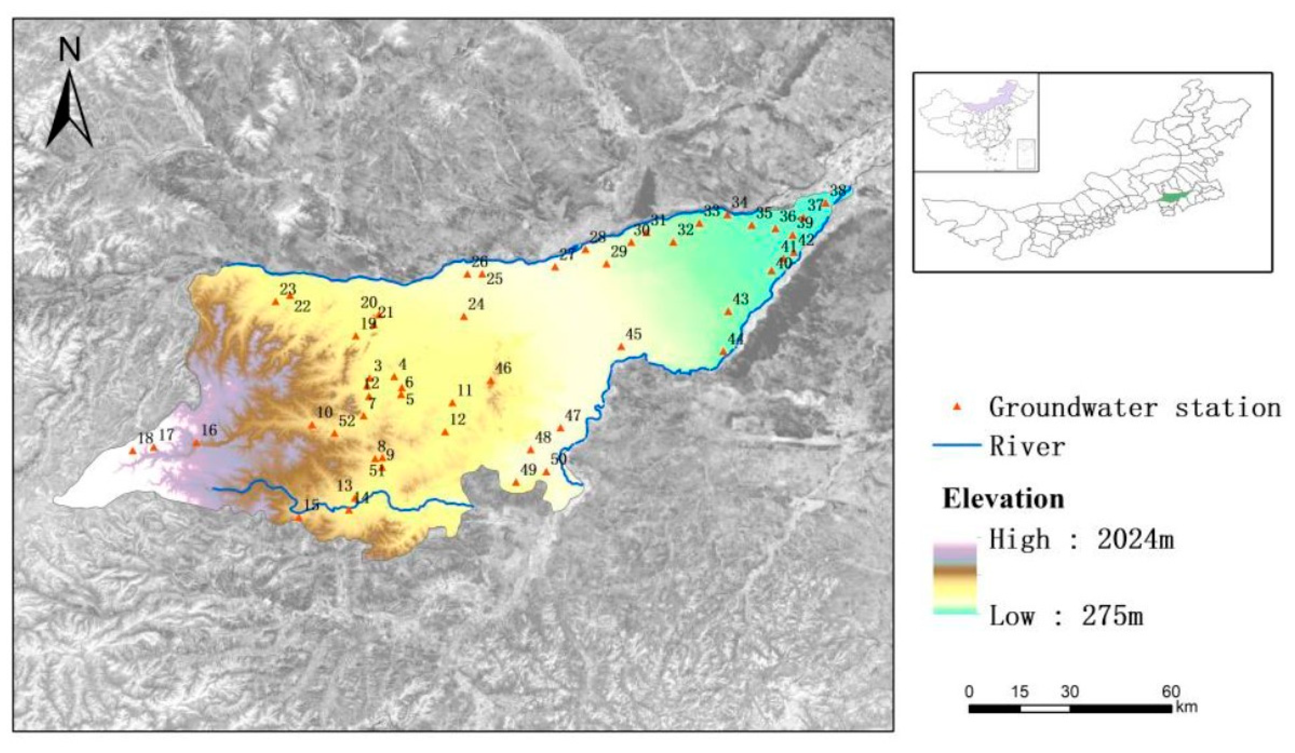
Wengniute Banner is one of the severe water-deficient areas in Inner Mongolia. The water-deficient and ecologically fragile area accounts for more than 30% of the city’s total area and is a typical research area for key agricultural and pastoral zones (KAPZs) [19,20]. Due to specific natural geography and hydrogeological conditions, groundwater has always been an important source of water for the Wengniute Banner and played an important role in the development of the regional economy [19,20,21,22,23]. However, severe water shortage, coupled with long-term over-exploitation and a lack of groundwater resources has become an ecological “bottleneck” that constrains regional economic development [22]. Most researchers study the groundwater distribution mainly through two approaches. The first approach is the model mechanism for simulating the collection and convergence process of groundwater, such as the groundwater flow model [24], land surface process model [18], transient numerical model [25], global climate models [26], regional climate models [15], etc. The second approach is using a regression model to fit the groundwater data to find the law of spatial and temporal changes of groundwater [13,14]. Some researchers took a different approach and used qualitative sensing inversion methods to study groundwater characteristics qualitatively [27]; Kotowski and Satora used the Kruskal–Wallis test (K-W) for the spatial analysis of the concentrations of selected ions in groundwater. The K-W test is the non-parametric equivalent of the one-way analysis of variance. There are also many other papers presenting a similar, modified or other methodological approach [28,29,30,31]. Rahmati investigated the delineation of groundwater potential zone based on Dempster–Shafer (DS) theory of evidence and evaluate its applicability for groundwater potentiality mapping [32]. Al-Ruzouq is based on the weighted overlay analysis of the analytic hierarchy process and is supported by random forest machine learning technology to explore the potential groundwater zones in the northern United Arab Emirates [33]. Salman applies statistical and geostatistical methods to monitoring data sets to assess the pollution risk of soil and shallow groundwater [34]. However, these models and methods do not comprehensively analyze the process of collection and convergence, and the temporal and spatial variation of groundwater is affected by many factors [35]; therefore, it is urgent to find a way to effectively reflect the temporal and spatial variation of groundwater; then, the characteristics and laws of groundwater volume changes under the combined action of various driving factors could be analyzed.
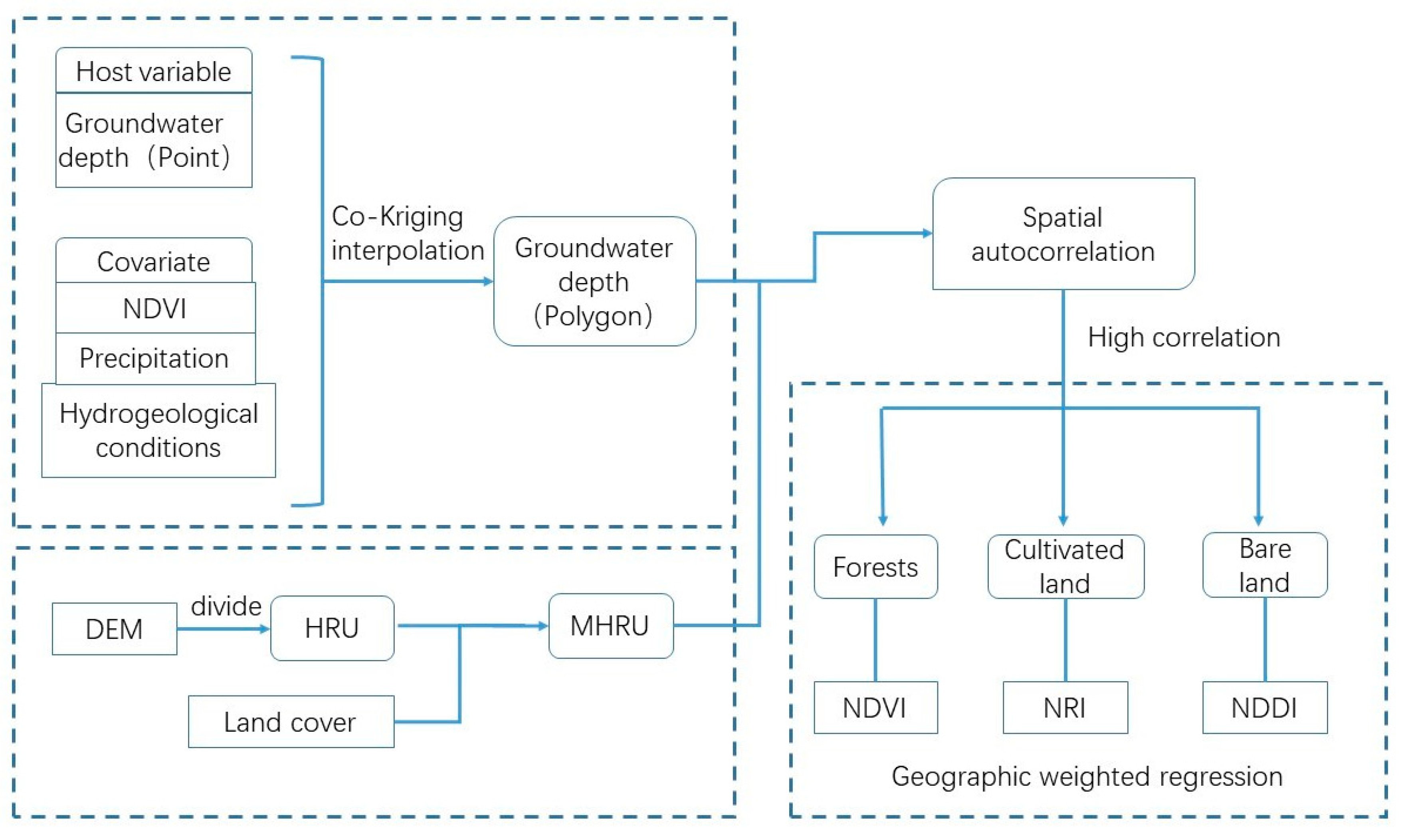
In this paper, the groundwater depth is presented in the spatial range using cokriging interpolation and used as the main variables including 2005, 2009, 2013, and 2017. The covariates consist of the normalized difference vegetation index (NDVI), precipitation, and hydrogeological conditions for the corresponding year. Cokriging interpolation is based not only on the spatial geographic characteristics of groundwater depth data but also on the various factors affecting groundwater depth. The synergistic kriging interpolation results have certain limitations in the response relationship between groundwater and spatial characteristics. Subsequently, the hydrological response unit theory is used to convert the grid units in the space into vector units, so that the data are closer to reality and conforms to the state of the recharge and confluence of groundwater depth. The research goal of this paper is to explore the characteristic information of groundwater burial depth in the KAPZs and analyze its distribution law on the scale of space and evolution characteristics on the scale of time. In combination with remote sensing band information, the relationship between different types of groundwater and the buried depth of the groundwater is clarified. The minimum response units (MHRUs) that provide the groundwater depth interpolation results are spatially analyzed by the spatial autocorrelation method to study the differentiation law and characteristics of Wengniute banner on time and space. The goal of this method is to provide a realistic reference value for the rational development and utilization of groundwater resources, as well as local land planning and utilization and agricultural development planning. The MHRU is an improved hydrological response unit (HRU) with the same hydrological characteristics and is divided according to factors such as soil, slope, and vegetation in the basin. The research method based on the MHRU could play an important role in the field of rational allocation of water resources in the Earth’s key zones and water environment risk assessment. The concept of MHRU was applied to the simulation of groundwater depth and scattered point data were simulated for the entire study area. Spatial autocorrelation studies the spatial distribution characteristics of groundwater depth and explores the spatial correlation model, which can better analyze the spatial autocorrelation characteristics of groundwater depth in soil from a regional perspective.
The innovations of this study are: (1) The cokriging interpolation method was used to simulate the spatial distribution of groundwater depth. (2) The accumulation characteristics of groundwater are analyzed by obtaining the spatial distribution of groundwater depth. (3) The groundwater area with aggregation characteristics was analyzed by remote sensing the waveband of land type to determine the quantitative relationship between groundwater depth and waveband combination. Based on the results of this study, by obtaining groundwater information, the groundwater depth in the space can be calculated through collaborative kriging interpolation. Without groundwater information, it can be quantitatively retrieved through remote sensing bands, and groundwater depth information with a certain accuracy can also be obtained. This study has certain limitations. The accuracy of the model is higher in farming and pastoral areas with low vegetation coverage and it is also suitable for arid and semi-arid areas. The error is larger in high altitude alpine mountains and dense forests with high vegetation coverage.

2. Materials and Methods

2.1. Study Area

2.1.1. Basic Situation

Wengniute Banner is located in the central part of Chifeng City, Inner Mongolia Autonomous Region. It is connected to Aohan Banner and Songshan District of Chifeng City in the south, Keshiketeng Banner in the west, Linxi County, Balin Right Banner, and Aru Kerqin Banner in the north, and Neiman Banner in Tongliao City in the east. Wengniute Banner is located between 117°49′–120°43′ east longitude and 42°26′–43°25′ north latitude [21,22]. The west is an alpine platform, the middle is a hilly area with gentle undulations and mountains and rivers, and the east is the Horqin Sandy Land. Within the study area, there are both low-lying marshes between the sand and the meadows and plains formed by the impact of the water flowing from the intersection of the Laoha River and the Xilamu River. It forms the complex terrain known as the “Five Sands and Four Hills and One Field” [20]. The total area studied is 11,889 km2. The area belongs to the temperate semi-arid continental monsoon climate with 2850–3000 h of annual sunshine duration, 5.5–6.4 °C of annual average temperature, and 300–400 mm of the average annual precipitation. The precipitation in the western mountainous area is 400 mm, the central hilly area is 360 mm, and the eastern bare ground area is 300 mm. The spatial and temporal distribution of groundwater in the area is extremely uneven, depending on atmospheric precipitation recharge, farmland irrigation, dry channel infiltration, and reservoir seepage [20,23,36,37].

2.1.2. Hydrogeological Conditions

The study area belongs to the first-level tectonic unit of the North China plate and is bounded by the Chifeng–Kaiyuan deep fault. It is divided into two second-level tectonic units, the continental margin of the northern part of North China and the North China block. The platform area is small, and the folds are not obvious. The scale, occurrence, nature, and types of fault structures are complex and changeable. According to their geological types, they are divided into fault basin boundary faults, general faults, and volcanic structure faults. The basin boundary fracture is the main boundary that divides the groundwater system or subsystem. Tensile faults and partial compressive faults in the bedrock area can store water, conduct water, or store or conduct water on one side, and loose layers or shallow overburden areas and rock formations with fractured pore water are the main water-bearing horizons.
Based on the occurrence conditions and hydraulic characteristics of groundwater, the main types of aquifers (groups) in this area include loose rock pore water, bedrock fissure water, and fracture zone vein water. The spatial distribution of water richness and water quality of each aquifer is quite different.
Loose rock pore water aquifers are mainly distributed in river valley plains and loess hilly areas. Depending on the lithology, structure, and thickness of the aquifer, their water richness varies in different regions. The first and second terraces on both sides of the Jiaolai River, Yangxu River, Mengke River, Shaolang River, and Laoha River Valley are rich in water. The water in bedrock fissures includes layered rock fissure water and massive rock fissure water. The fissure water of layered rocks is distributed in the low and middle mountains and low hilly areas in the east and middle. The vein-like water aquifers in the fault zone are mainly distributed in the low mountain and hilly area in the southern part of the area. The fault structure is relatively developed, with east–west, north–east, and north–west faults. In the fault structure, several groups of fracture zone rocks are relatively broken. The fissures are developed, the opening is good, and the filling is less.

2.2. Data Sources

There are 40 monitoring sites in Wengniute Banner monitoring well (see the Appendix A Table A1), as shown in Figure 1. The monitoring wells have been observed since 2005, and the observation data until December 2017 have relatively complete information. When monitoring groundwater data, follow the groundwater monitoring well construction specification (DZ/T 0270-2014) and the “Technical Specification for Long-term Groundwater Dynamic Observation (MT/T 633-1996)”. Regarding the accuracy of water level monitoring, when measuring the static water level, the maximum error of two consecutive measurements should not be greater than ±1 cm/10 m. Every time the water level is monitored, whether the observation well has ever been pumped is recorded, and whether it has been affected by the pumping of nearby wells. The Landsat TM images in 2005 and 2009 and Landsat OLI images in 2013 and 2017 (http://www.gscloud.cn/) were selected to perform band synthesis, image enhancement, and geometric correction using Environment for Visualizing Images (ENVI) 5.1 software. ENVI, as a complete remote sensing image processing platform, is the flagship product of Exelis Visual Information Solutions in the United States. Then, through the establishment of interpretation impact and field investigation, the land-use status and NDVI in 2005, 2009, 2013, and 2017 were obtained. The DEM (digital elevation model) was downloaded from the Geospatial Data Cloud (http://www.gscloud.cn/). Data from the precipitation site near Wengniute Banner were obtained; data for Bahrain Zuoqi, Linxi, Wengniute Banner, Baoguotu, and Chifeng can be obtained from the National Meteorological Information Center (http://www.nmic.cn/). The soil lithology, soil particle size, topography, and other data in hydrogeological conditions were obtained from the Chengdu Institute of Mountains, Chinese Academy of Sciences.

2.3. Pretreatment

The groundwater depth data for the summer of 2005, 2009, 2013, and 2017 were selected as the basic data for spatial interpolation (Table 1).
The seasonal changes in the depth of groundwater at various points are shown in Figure 2. The seasonal changes are more obvious. Due to more rain in spring and summer, the depth of groundwater is generally higher than in autumn and winter. The error of seasonal variation of groundwater depth at most points is within ±2 m, but from the data in the figure, the difference between the general minimum and maximum is too large, and the average value can accurately represent the characteristics of groundwater most of the time. Due to the limitations of the experiment in this study, it is impossible to use all the data for the year. The maximum and minimum values are not too different between months; therefore, the average value of the groundwater depth in a year is selected to represent the characteristics of the groundwater depth.

2.4. Data Processing

In this paper, groundwater depth data were used as the host variable, and NDVI, precipitation, and hydrogeological conditions were used as covariates. The groundwater depth data within the study area were obtained using cokriging interpolation. At the same time, MHRU was divided according to DEM and land cover. Using MHRU as the carrier, through spatial autocorrelation analysis of three types of land with obvious spatial aggregation characteristics: forest land, cultivated land, and bare land. Then, the corresponding remote sensing inversion band index NDVI, net relatedness index (NRI), and normalized difference drought index (NDDI) were selected for the geographically weighted regression (see Figure 3). This model is mainly suitable for bedrock and loess hilly areas. The accuracy is higher in areas where the aquifer types are loose rock pore water, bedrock fissure water, and fracture zone vein water. Fine-grained lithological combinations and arid and semi-arid areas with poor diving are more suitable.
The originality of this paper is to construct a spatial simulation method of groundwater depth and to present groundwater information in space through interpolation analysis. Compared with traditional kriging interpolation, cokriging interpolation combines hydrogeological conditions, precipitation and vegetation coverage, and other influencing factors, highlighting anisotropy in the interpolation model, making the simulation results more consistent with the actual groundwater cycle characteristics, and at the same time, also solving the unrealistic limitation of the traditional interpolation model due to single variable interpolation. At the same time, in subsequent research, a regression model between groundwater depth and remote sensing bands of different land types was constructed through geographically weighted regression. Considering a situation where researchers lack groundwater data, groundwater depth information can be quantitatively simulated; however, because the construction of the groundwater spatial interpolation model uses local hydrogeological information, this model is more suitable for arid and semi-arid farming-pastoral interlaced areas, especially in areas with finer lithology and poor diving.

2.5. Methods

2.5.1. Cokriging Model

As shown in Figure 1, the groundwater depth is distributed in the form of point data. To analyze the temporal and spatial differentiation of groundwater depth (annual average groundwater depth) quantitatively and qualitatively, it is necessary to spatially present the groundwater depth data. Compared with other interpolation methods, cokriging is a strong spatial correlation between host variables interpolated within a region and multiple attribute variables [25] and adds multiple regionalized covariate variables based on the main variable. The correlation is constructed by fitting the model, which is helpful to estimate the distribution of dependent variables [38,39,40].
Cokriging interpolation simulates the distribution of groundwater depth, which uses the vegetation characteristics, precipitation, and hydrogeological conditions to influence the static characteristics of groundwater depth as covariates. The distribution of topography and the coverage of surface vegetation, which can reflect the soil’s water-fixing capacity, have a crucial impact on the recharge range, mode, and degree of groundwater depth. The groundwater depth is generally stable in places with high vegetation coverage and has not changed much over the years, but it has affected the time variation characteristics of groundwater depth.
Three major factors affect groundwater:
  • The terrain influences the convergence of groundwater, which is the most significant variable affecting the spread of groundwater.
  • Hydrogeological conditions affect the depth of groundwater.
  • Precipitation is the main source of groundwater runoff and hydrogeological conditions are an important carrier for groundwater diversion.
These three jointly determine the spatial variation characteristics of groundwater depth; therefore, this paper selects NDVI, precipitation, and hydrogeological conditions as covariates, and performs cooperative kriging interpolation on groundwater depth.
In ArcGIS10.4 (ESRI, Redlands, CA, USA, 2016), ordinary kriging interpolation, simple kriging interpolation, pan kriging interpolation, and extract kriging interpolation were selected for interpolation comparison. Ordinary kriging interpolation is mostly used for the unbiased estimation of a single variable. Pan kriging interpolation needs to know the overall trend of the entire interpolation space. Extract kriging interpolation is a nonlinear interpolation model. The most effective interpolation method can be chosen through parameter comparison.
The impact factor data corresponding to the covariate K of the collaborative regionalization is Z k (x), (k = 1, 2, …, x), where k 0 is the main variable groundwater depth change rate. The mathematical expectation of the rate Z k 0 ( x i ) (i = 1, 2, 3, …, n) of change of the buried depth at each groundwater survey site exists and is a fixed value m k 0 .
Z V k 0 is the average value of the underground burial depth change rate k 0 .
Z V k 0 = 1 V k 0 V k 0   Z k 0 ( x ) d x
Z α k is the average value on the carrier V α k :
Z α k = 1 V α k V k 0   Z k ( x ) d x
The estimated rate Z V k 0 * of groundwater depth change over the entire region is a linear combination of the effective values of the k coordinated regional variations.
Z V k 0 * = k = 1 K α k n k μ α k Z α k
In the formula, Z V k 0 * is the estimated value of the change rate of the buried depth of the main variable; μ α k is the cokriging interpolation factor weight coefficient; Z α k is a synergistic region variable.
In this paper, the covariates are DEM, hydrogeological conditions, and NDVI, respectively using u i ( i = 1 , 2 , n ) , v j ( j = 1 , 2 , m ) , p s ( q = 1 , 2 , r ) to represent:
Z V k 0 * = i = 1 n a i u i + j = 1 m b j v j + q = 1 r c s p s
In the formula, a i , b j , c s are the precipitation, hydrogeological conditions, and the weight coefficient of the NDVI, respectively [41,42,43,44].
Interpolation analysis can present the buried depth of groundwater in space and simulate the buried depth of groundwater at a specific location; however, kriging interpolation has low accuracy when there are fewer original points and uneven distribution; therefore, the use of cokriging interpolation combines multiple factors that affect the depth of groundwater to improve the model to improve the accuracy of groundwater depth prediction.

2.5.2. Minimum Hydrological Response Unit

The result of groundwater depth is spatially presented as raster data, which is interpolated according to the cokriging interpolation; however, the division unit of groundwater depth is not similar to the regular shape of the grid in the actual situation due to the spatial difference of multiple factors and the irregularity of land use types; therefore, in this paper, we borrow the concept of MHRU to transform raster data into vector data, so that the subsequent spatial analysis would be more suitable for the actual situation in the study area.
The minimum hydrological response unit (MHRU) is based on the hydrological response unit (HRU), which is the basic unit of simulation in the SWAT (Soil and Water Assessment Tool) model [45,46]. The minimum response unit is defined by land use, soil type, and slope based on HRU. Combined with the moderate index method, the adaptive index threshold system is constructed, and the sub-basin can be better divided by hydrological analysis based on DEM. Based on the generation of the sub-basin, the hydrological response unit is determined and relevant research is carried out at this scale [47,48,49].
The basin calculation can be achieved using hydrological analysis in ArcGIS. The D8 single flow algorithm principle defines the eight directions around each grid unit of the DEM [50,51]. Assuming that the rain falls on a certain grid in the terrain, the water flow of the modified grid will flow to the grid with the lowest of the eight grid tops. If the maximum descending direction of multiple cell grids stays the same, then the adjacent cell range should be expanded until the steepest descent direction is found [52,53,54]; therefore, it is feasible to use the hydrological response unit to express the variation of groundwater depth.
The HRU is delineated using the hydrological analysis tool in ArcGIS. The watershed delineated by DEM can only represent one feature of the terrain. There are a variety of land types in the same watershed, and the groundwater content of the storage is also different; therefore, the land cover data are used to divide the watershed twice, and small patches of the boundary are combined to obtain the final MHRU. The land cover and watershed division of each MHRU, which can evaluate the groundwater depth and analyze the spatial and temporal differentiation of groundwater depth, are different and have unique characteristics.
First, we assign a value to the divided MHRU. Then, through the partition module in the analysis tool, the average groundwater depth of each hydrological response unit in the space can be statistically analyzed, and then space depth can be analyzed through the attribute connection.

2.5.3. Spatial Autocorrelation

It is necessary to conduct a qualitative and quantitative study on the spatial and temporal differentiation characteristics of groundwater by coupling the well-defined MHRU and groundwater depth interpolation results [55,56]. The groundwater depth value is presented through the MHRU, and the results are subjected to spatial autocorrelation analysis. Spatial autocorrelation refers to the potential interdependence of observational data between variables in the same distribution [57]. Tobler once pointed out that “the first law of geography: anything is related to something else, but things in the neighborhood are more relevant than things in the distance.” Statistically, correlation analysis can be used to detect whether there is a correlation between the changes of the two phenomena—it is the same attribute variable of different observation objects, which is called autocorrelation [58,59,60,61]. The parameters describing spatial autocorrelation include global autocorrelation and local autocorrelation. Local autocorrelation was used in this study to express the recharge and convergence process of groundwater.
Local spatial autocorrelation is a correlation index used to measure the extent to which a local spatial unit affects the spatial autocorrelation of the overall study [62]. Local spatial autocorrelation represents the degree of correlation of the specific hydrological response unit with the groundwater depth of the adjacent hydrological response unit and is calculated as follows [63,64]:
I = n ( x i x ¯ ) j = 1 m W i j ( x j x ¯ ) i = 1 n ( x i x ¯ ) 2
where m is the number of hydrological response units adjacent to the hydrological response unit i .
Based on the groundwater depth data for several years, the spatial autocorrelation analysis can be performed according to the area divided by the minimum hydrological response unit. In this way, the trend of groundwater depth in the past two decades is obtained and presented in the form of spatial plots, and the clustering degree and related situation of groundwater depth in the actual situation can be analyzed.

2.5.4. Geographically Weighted Regression

Based on the previous period, the spatial and temporal differentiation of the groundwater depth was qualitatively analyzed using spatial autocorrelation analysis. In the process of the confluence of groundwater depth, the land cover type is an important influencing factor. Through geographically weighted regression, the response mechanism of recharge and convergence processes of different land types and groundwater depth was quantitatively analyzed. The specific remote sensing band index was selected to represent the land type that has a great influence on the groundwater depth and is represented by the MHRU. A geographically weighted regression model of the index corresponding to different land types and groundwater depth was constructed. Combined with spatial characteristics, quantitative analysis of the influence of surface characteristics of different soils on groundwater depth [65,66,67] was then carried out.
Geographically weighted regression is based on the ordinary linear regression model, which embeds the spatial position of the data into the regression equation. The formula is as follows:
y i = β 0 ( u i , v i ) + k = 1 P β k ( u i , v i ) x i k + ε i
where ( u i , v i ) is the sampling point i coordinate, β k ( u i , v i ) is the kth regression parameter at the sampling point i , which is a function of the geographical position, and the weight function is obtained in the estimation process.
The Gaussian kernel function to determine the bandwidth is as follows [68,69,70]:
ω i j = e x p ( ( d i j b ) 2 )
where b is a non-negative attenuation parameter describing the functional relationship between weight and distance, called bandwidth. The larger the bandwidth, the slower the weight is attenuated with distance, and the faster the weight is attenuated.

3. Results

3.1. Cokriging Interpolation of Groundwater Depth

Based on the geostatistical guidance tool in ArcGIS, the groundwater depth was analyzed by collaborative kriging interpolation, and then different covariance functions for function fitting accuracy analysis were selected. The comparison of 11 functional models in the ring model, spherical model, three-ball model, K-Bessel model, J-Bessel model, and stability model is shown in Table 2. In the accuracy verification of the covariance model, the stable model has the best effect of the 11 models.
To verify the effect of cokriging interpolation in different experimental well densities in the study area, 10 sets of training samples were selected for comparison and verification, of which three samples were located in the eastern region, three samples were located in the central region, and four samples were located in the western region (Figure 4). The samples in the eastern region show that the groundwater depth is shallower, and the model accuracy is higher. The samples in the central region show that the groundwater is buried deep, and the model accuracy is average. The samples in the western region show that the depth of groundwater is deeper, and the accuracy of the model is higher (Table 3).

3.2. Spatial Distribution of Groundwater Depth

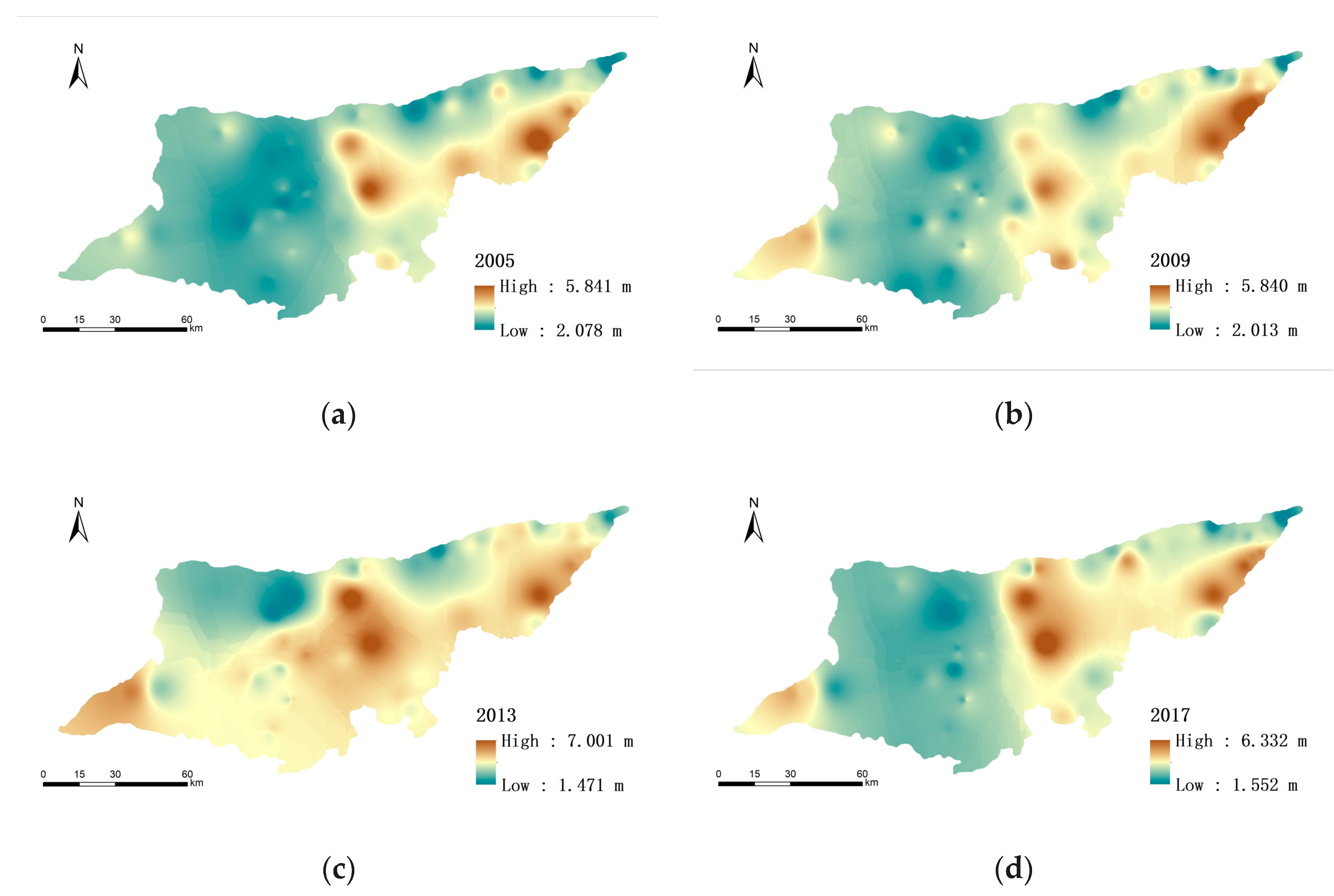
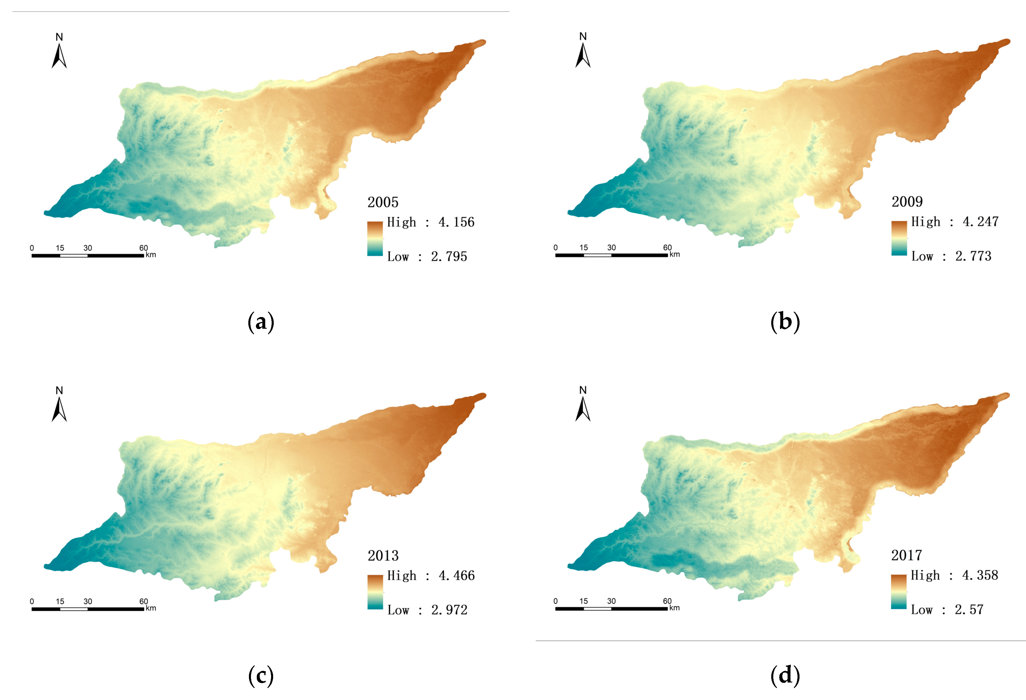
Compared with a single groundwater depth as an interpolation factor, the cokriging interpolation makes the result smoother in space, and has no abrupt point-like aggregation characteristics, which can better reflect the spatial distribution of groundwater (Figure 5 and Figure 6). The results are more obvious in spatial differentiation. Among them, the difference in groundwater depth in the study area is obvious, and the depth of groundwater is greatly affected by land-use type. In the four years, the groundwater depth on the east side is relatively large, mainly distributed in the farmland centered on Shengli Village in the lower reaches of the Xilamulun River and the dune wasteland near Dule Benji. The central and eastern parts of Wengniute Banner are mainly plain dunes, covered with vegetation such as wild grasses. Years of drought and lack of water have resulted in lower groundwater depths within this range. Although large areas of farmland are adjacent to the Xilamulun River and there is a certain amount of crop cover, the water demand is also huge due to intensive crop planting. Residents generally dig wells around the farmland to irrigate the land nearby. The amount of water causes the groundwater depth in large-scale farmland to be generally deeper. The farmland concentration area in the lower reaches of the Laoha River is similar. The area with better groundwater depth is mainly distributed in the west. According to the results of four years’ interpolation, the vegetation coverage in the western mountainous areas is relatively high, and there are many tall and dense shrubs. The diversity of plants with improved, developed root systems and good soil environment are all conducive to the maintenance of soil moisture. A large amount of water could be fixed in the soil by the rainfall; therefore, the groundwater depth is generally shallow in the eastern part of the study area. The severely water-deficient areas in Wengniute Banner are mainly low-mountain hills, loess hills, and loess terraces, and their geology, geomorphology, and hydrogeological conditions are extremely complex. By analyzing the geological and hydrogeological environment of groundwater in the study area, the water quantity is abundant and the water quality is good, which can meet the needs of human and animal life, industry, agriculture, and animal husbandry in the area; however, water shortages are more serious in low hills, loess hills, and loess plateau areas. Factors such as precipitation, topography, lithology, and groundwater circulation are the main reasons for the serious water shortage in this area. Stratum lithology and neotectonic movement are the decisive factors affecting the enrichment of groundwater.
Comparing the groundwater depth interpolation results in 2005, 2009, 2013, and 2017, the variation law of groundwater depth in time was analyzed with four years as the boundary. In 2005, the groundwater depth was between 2.7 and 4.1 m, and the overall distribution was relatively uniform. The groundwater depth was mainly distributed in the dune area of the northeastern part of the study area, and the groundwater depth in most areas exceeded 3 m. It indicates that groundwater diversion and convergence are relatively smooth in the past year, and there are few obstacles in the transmission process. In 2009, the groundwater depth was between 2.7 and 4.3 m, and its situation was not significantly different. The area with large groundwater depth was concentrated in the northeast and southern farmland. It indicates that the groundwater depth this year was greatly affected by location coupled with low precipitation. The groundwater depth in the river area and the farmland area is relatively close, and the farmland needs excessive extraction of groundwater for agricultural irrigation. In 2013, the groundwater depth was between 2.9 and 4.5 m, and the difference was small. The groundwater diversion and convergence process in the soil was unobstructed, but the overall groundwater depth was low, and the distribution trend was similar in 2009. The precipitation is relatively average but not sufficient, and surface runoff plays a major regulatory role. In 2017, the groundwater depth was between 2.5 and 4.4 m, which was relatively evenly distributed. Based on the results of the above four years, it can be concluded that the average value of groundwater depth will not fluctuate too much in a short period, but local areas such as northeast farmland and central and eastern dunes are still changing significantly. The groundwater depth is greatly affected by factors such as precipitation in the current year.

3.3. Spatial Autocorrelation Analysis

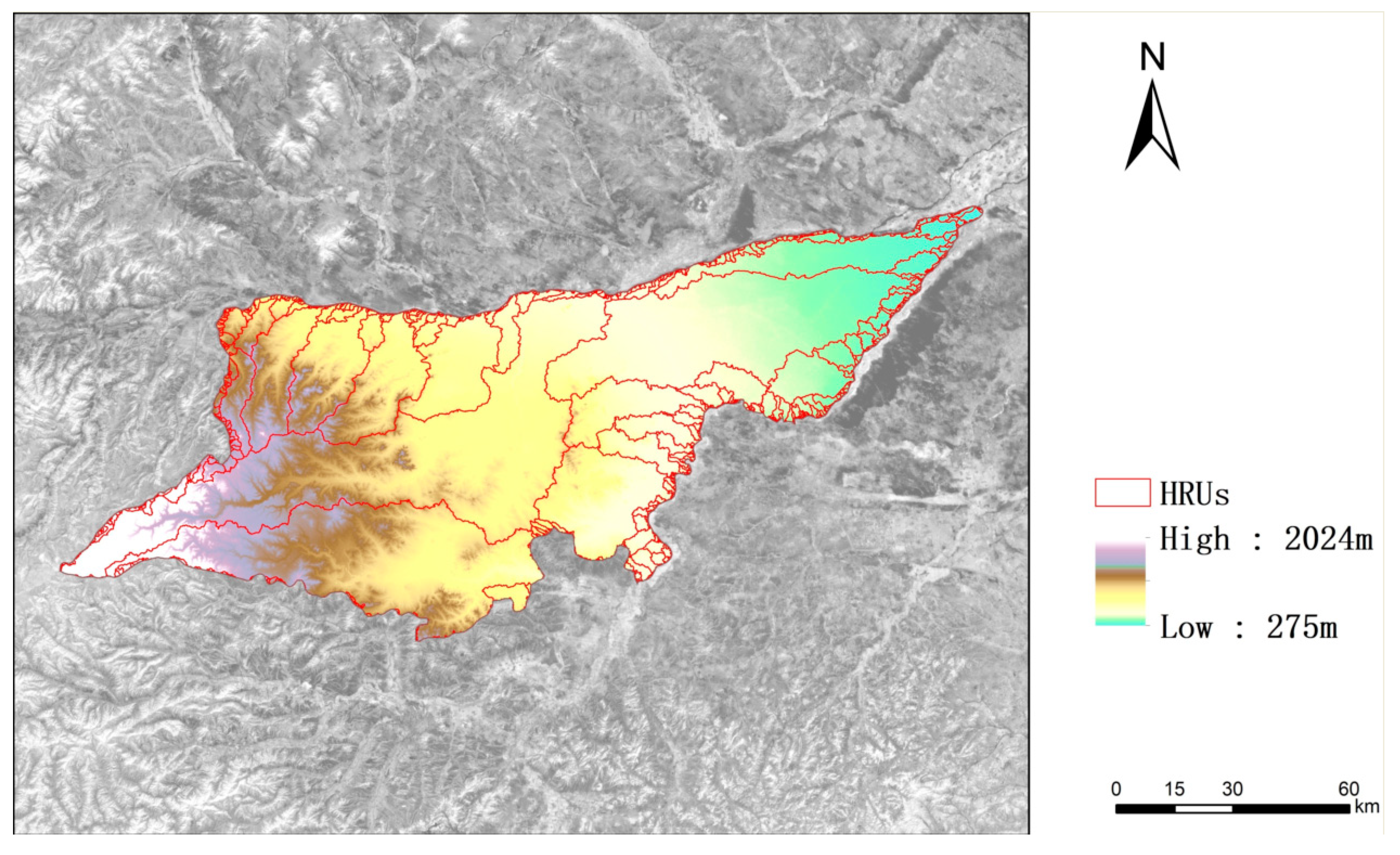
According to the hydrological analysis based on the DEM data in ArcGIS, 6614 HRUs are obtained, as shown in Figure 7. The traditional HRU has a large number of small plaques at the boundary, and the small plaques of less than 75 hectares are eliminated by the elimination tool, and 83 HRUs are obtained. The groundwater characteristics of HRU less than 75 hectares do not significantly differ in land type. The HRU is only based on the topographical division of the study area. The spatial division of the groundwater depth is also affected by the type of land use. Cultivated land, forest land, and construction land have different groundwater diversion and confluence and impacts. Different land types have characteristics such as soil types, vegetation coverage, soil water content, and water use; therefore, the hydrological response unit based on the topography is divided according to the land-use situation. After the division, the small shift is eliminated, and finally, 551 MHRUs are obtained. The MHRU represents different land-use types and groundwater confluence directions, which is of great significance for spatially presenting the recharge and convergence of groundwater depth. The response unit is divided according to the actual situation. The transmission of groundwater depth is not bounded by a fixed grid cell size, and the MHRU is a more realistic response unit constructed according to the actual situation. A single MHRU has consistent groundwater depth and spread with the same type of land use, approximate soil type, vegetation cover, terrain slope characteristics, and groundwater flow direction; therefore, the analysis of the spatial differentiation law of groundwater depth based on the MHRU is highly feasible, scientific, and implementable.
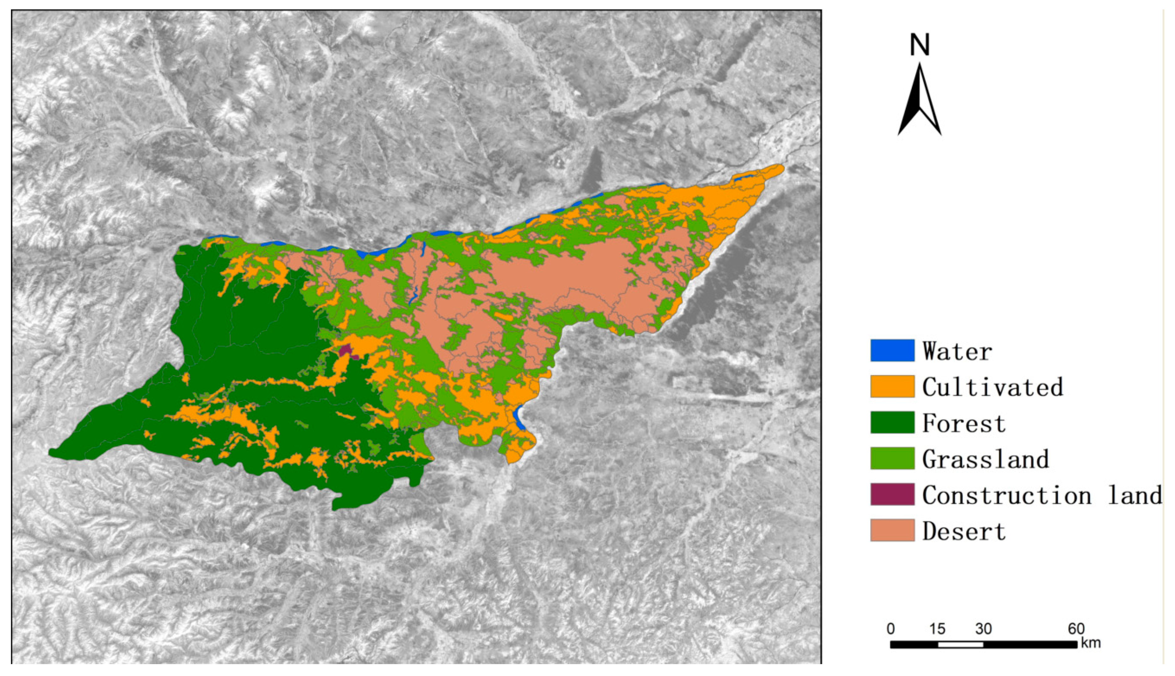
The distribution of the MHRUs in the study area is shown in Figure 8. Different types of MHRUs have certain distribution characteristics. Among them, 50 min response units of forest land are distributed in the west and southwest of Wengniute Banner, and there are national highways as boundaries. The west of the national highway is mainly forest land, and the elevation is generally above 1000 m. The distribution of MHRUs in forestland is relatively concentrated in one large area. In the forest, the aggregation characteristics of the MHRU are prominent, and the groundwater depth recharge and convergence characteristics are consistent. The distribution of water bodies in the study area is also concentrated. The MHRU is divided into the main distribution of water in the Xilamulun River Basin in the north and the Hongshan Reservoir in the lower reaches of the Laoha River. The MHRUs of water are divided into 26 sections with small areas. The MHRUs of cultivated land are divided into 158 sections with small areas, scattered distribution, and unspecific characteristics. One MHRU for construction land was obtained and is located in the city center of Wengniute Banner. There are 230 MHRUs for grassland, which are the most common of the six land types, and have the smallest distribution unit with the widest distribution. The only characteristic is the distribution around the bare ground area. There are 86 MHRUs in the bare ground, which are mainly distributed in the middle and east of the study area. Among them, five are larger and more concentrated. The law of groundwater diversion in such minimum response units should be most pronounced.
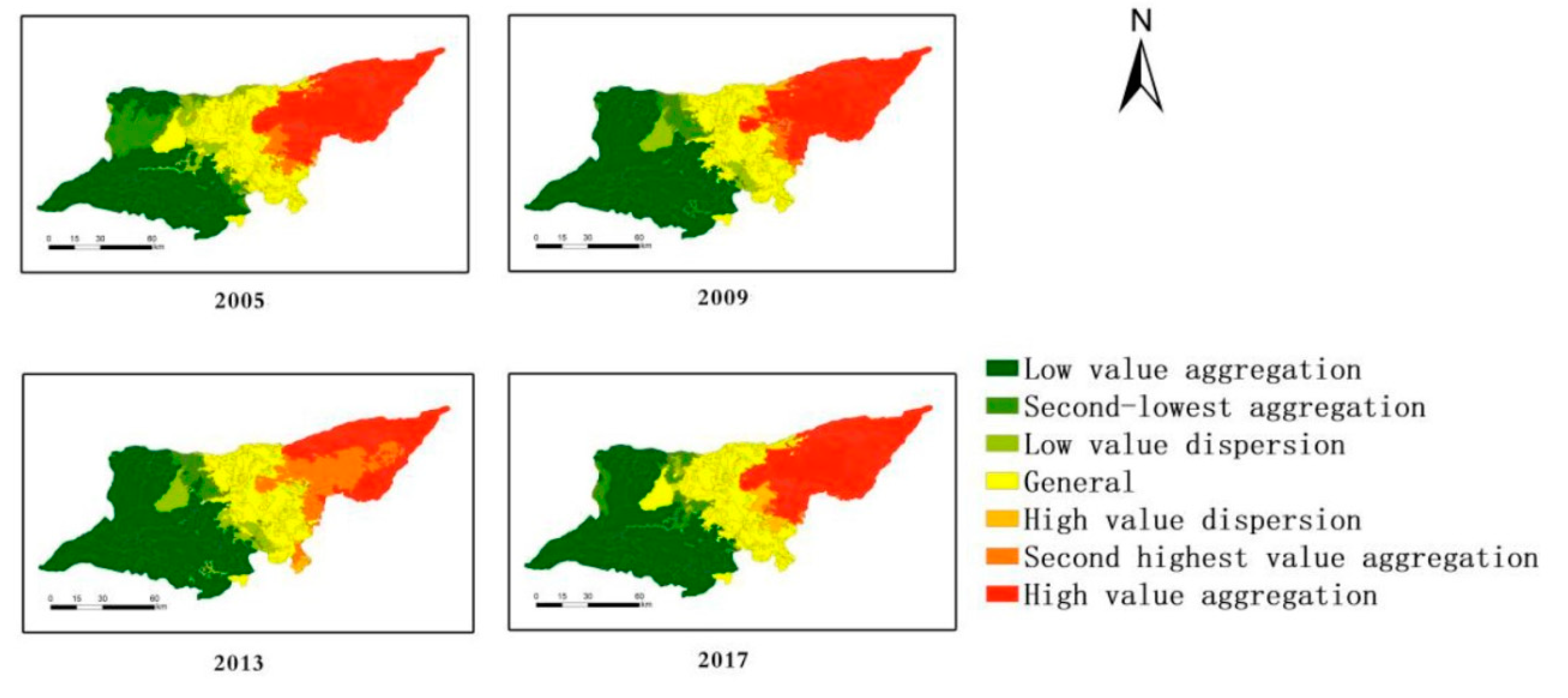
The results of collaborative kriging interpolation are assigned to the MHRU, and then the local autocorrelation under the spatial autocorrelation in the spatial statistical tool is used to analyze the distribution and evolution of groundwater depth in four years. The spatial autocorrelation results are shown in Figure 9.
The spatial autocorrelation characteristics presented on the MHRU by four-year groundwater interpolation can be obtained. The groundwater burial depth of the 135 MHRUs in the northeast of the study area showed high accumulation characteristics from 2005 to 2017. The characteristics of high aggregation are spatially expressed as high-value areas within the range—specifically a combination of significant aggregation and a degree of homogeneity among the values in the range. Most of the high-gathering areas are arable land, and the gathering characteristics are obvious, indicating that within a large area of farmland, groundwater connectivity is better. The standardized planting crops are more consistent in water demand and water fixing capacity, combined with relatively flat terrain, making this part of the contiguous area appear as a high-value gathering area. The dune plains in the middle and east of the study area also exhibited large-scale high-value accumulation, which showed non-large-value accumulation characteristics in individual years, indicating that the spatial distribution of groundwater depth in the plain dune areas is very irregular and not stable enough. There are some areas in the plain dune area where the groundwater depth is relatively high, and there are obstacles to groundwater interaction. The flow and recharge of groundwater are affected to a certain extent, and the aggregation characteristics are not as obvious as those of cultivated land. There are 114 MHRUs in the western part of the study area, all of which are low-value aggregation areas in four years. Among them, the MHRUs are divided by forest land. The terrain in the west is too large, in the same area, the number of MHRUs in low-value aggregation areas is less than that in the east. From the distribution of the low-value gathering area, it can be found that it is mainly distributed in the range of forest land, rather than the MHRU with a high groundwater depth such as water body. It shows that the buried depth of groundwater can show large-scale accumulation in the mountainous area in the west, and the well-developed tree roots in the forest have a strong water conservation function, which promotes the accumulation and confluence of groundwater. There is no obvious accumulation characteristic in the middle of the study area, no regular characteristic for the distribution of groundwater burial depth high- and low-value areas, and no accumulation phenomenon. Bare ground and grassland are mixed in the range and the groundwater confluence process in these two types of areas is hindered greatly.
The correlation between high-value aggregation areas and low-value aggregation areas is greater than 99%. The correlation between the second-highest aggregation area and the second-lowest aggregation area is greater than 95%. The correlation between the high-value dispersion area and the low-value dispersion area is greater than 90%. Comparing the spatial differentiation characteristics of groundwater depth in four years, it is clear that there is little difference in the change of the low-value accumulation area in the MHRU of the woodland in the western mountainous area; however, in the short term, the low-value gathering areas showed obvious aggregation characteristics, and are mainly distributed in areas where forest land is concentrated. Some sub-low-value accumulation areas and low-value dispersion areas gradually decreased or disappeared. The expansion of the forest land area caused the accumulation characteristics in the west to increase year by year. In the eastern part of the study area, the overall distribution and changes from 2005 to 2017 are similar to those in the west, except for 2013, when the changes in the east are weaker, and the characteristics of cultivated land aggregation are relatively stable. This shows that in recent years, the overall groundwater depth has displayed aggregation characteristics, and the groundwater confluence process has shown an orderly state.

3.4. Geographically Weighted Regression

The groundwater depth exhibits low-value aggregation characteristics in forest land, whereas the eastern cultivated and bare land areas exhibit high-value aggregation characteristics. Based on this, a geographically weighted regression analysis of the three land types and groundwater depth was performed, and NDVI, NRI, and NDDI were used to represent forest land, cultivated land, and bare land, respectively. NDVI, as a spectral band index, mainly reflects the characteristics of vegetation cover on the surface. For mountain forest land with high coverage, it is feasible to use NDVI as the index of the forest land. For the cultivated land in the study area, repeated tests on NRI, RVI (Ratio Vegetation Index), SAVI (Soil-Adjusted Vegetation Index), and GNDVI (Green Normalized Difference Vegetation Index) and other band indexes that can reflect the growth of crops could be implemented. NRI is the band that reflects the index of the nitrogen element of the crop. NRI can be used as the band index to reflect the cultivated land due to nitrogen fertilizer application. The central part of the study area is bare land and there are significantly large areas of desertification. NDDI effectively refers to the central bare land.
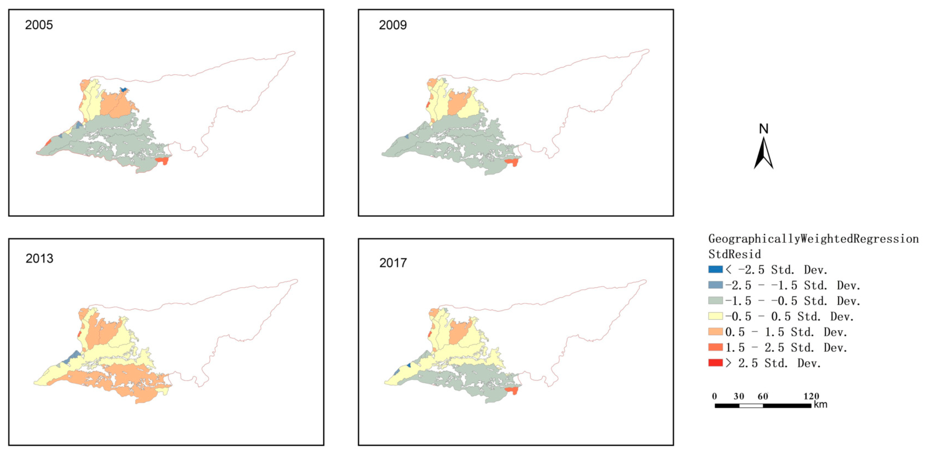
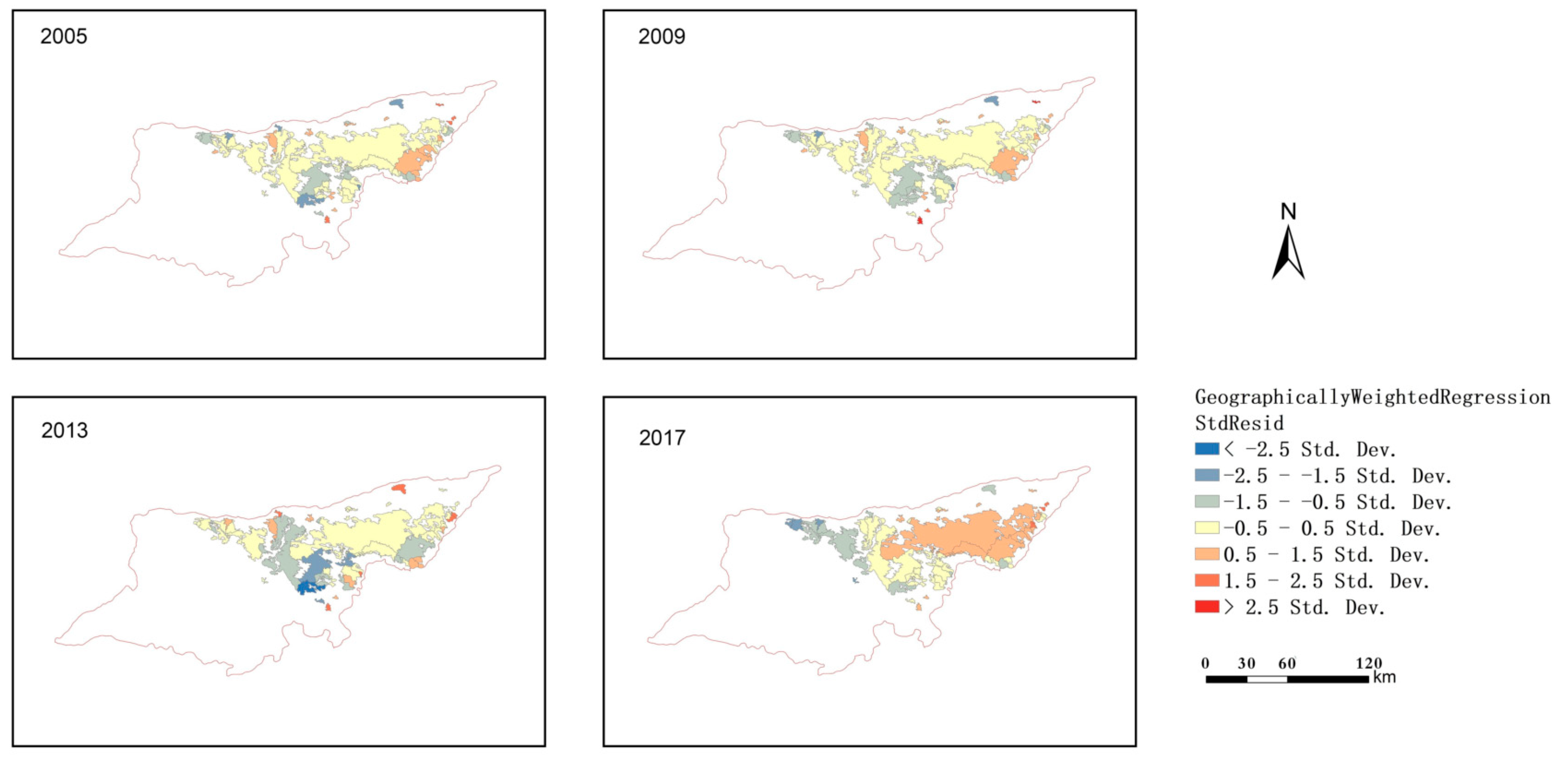
The results of the geographically weighted regression model of cultivated land in the four years of 2005, 2009, 2013, and 2017 are shown in both Figure 10 and Table 4, which shows the standardized residuals of the geographically weighted regression model of cultivated land and NRI. Patches with absolute residuals greater than 2.5 have a poor fitting effect. The closer the absolute value comes to 0, the better the fitting effect of the geographically weighted regression model. According to the graph and table analysis, the result of the geographic weighted regression of cultivated land is an improvement when compared to other methods. In four years, the coefficient R is greater than 0.8 and the R2 is greater than 0.75, which shows that the geographically weighted regression model has a strong correlation with the fitting of cultivated land NRI and groundwater depth. To further analyze the response mechanism, the standardized residual error is lower in the cultivated land in the middle of the study area, adjacent to the forest land in the west and the bare land in the middle and east, and the fitting effect of geographically weighted regression is also better than the other methods. The cultivated land in the southern and northeast corners of the study area is close to the boundary of the study area, resulting in the deviation of the fitting effect. The independent variables of geographically weighted regression of cultivated land in four years are between −4 and 10. The fitting coefficient of cultivated land and groundwater depth is mainly negative in the central and western parts of the study area. The higher the NRI, the smaller the groundwater depth. The cultivated land in the area is close to the river and the woodland in the western mountain area. The developed root system of the woodland allows for water conservation. The NRI coefficient of the cultivated land is mainly positive in the northeast of the study area. Although the cultivated land in this area is also close to the Xilamulun River, the large area of cultivated land requires more water, and the wasteland on the west side will also divert groundwater runoff. The water conservation function is not high enough to maintain a better groundwater environment in the case an increase in the range of water demand.
Figure 11 and Table 5 show the geographically weighted regression results of NDVI of forest land and groundwater depth. During 2005, 2009, 2013, and 2017, the NDVI of the forest land and the groundwater depth R2 were all above 0.6, and the adjusted R2 was above 0.5. NDVI and the groundwater depth have a strong correlation. The forest land is distributed in the western part of the study area, in which the residuals of some patches in the northeast, southeast corner, and west edge of the forest land are large, whereas the residuals in most other areas are within a normal function fitting interval for four years. The independent variables of the geographic weighted regression of forest land in four years are between −5 and 0.5, and the NDVI of vegetation coverage index is negatively correlated with groundwater depth. The areas with larger NDVI coefficients are mainly distributed in the smaller patches near the borders in the north and northwest of the woodland. It shows that in these areas, the impact of the tall trees is more obvious in the mountain area on the buried depth of groundwater. Part of the cultivated land in the southern woodland of the mountainous area affects the conservation of groundwater, and part of the groundwater converges to the cultivated land to supplement the water absorbed by the crops.
Figure 12 and Table 6 are the geographically weighted regression results of bare ground NDDI and groundwater depth. In 2005, 2009, 2013, and 2017, the bare ground NDDI and groundwater depth R2 were all above 0.72, and the adjusted R2 was above 0.68. NDDI and groundwater burial depth have a strong correlation. In accordance with the analysis above, the fitting result of the geographically weighted regression model of the bare ground area is very unstable, and the inter-annual variability is large. The standardized parameters of the middle and eastern bare ground in 2005 and 2017 are relatively large. In 2009 and 2013, the normalized residuals were relatively stable in this area. The fitting of the groundwater depth of the bare ground to NDDI is greatly affected by other factors. The independent variables of bare ground geographic weighted regression in the four years range from −2 to 6. The NDDI of the land drought index is positively correlated with the groundwater depth. The fitting coefficient of NDDI is greater than two in most bare land areas, and the impact of land drought on groundwater depth increases with the increase of NDDI.

4. Discussions

The KAPZs is an important component of the ECZ. Exploring its water cycle characteristics is the basis for optimizing the use of water resources. In this study, we used a variety of theories and methods such as spatial and statistical analysis under geography to construct a groundwater response unit for typical areas in KAPZs. The response unit could be used to study the trend and law of the collection and divergence of underground runoff in space, and analyze its distribution law in two dimensions of space and time. Furthermore, the intrinsic driving force of land cover could be determined through the construction of a geographic regression model combining spatial information.
To study the characteristics of groundwater burial depth in the KAPZs, the data of groundwater burial depth needs to be displayed in space first. Compared with ordinary kriging interpolation results, the use of cokriging interpolation methods combined with precipitation, vegetation coverage, and hydrogeological conditions interpolation results can effectively avoid errors caused by the spatial distribution of observation points (Figure 5 and Figure 6), to make the spatial distribution more regular, changes more gentle and more in line with the actual differentiation of groundwater depth. Seyed Hamid Ahmadi et al. used the Dalabu Plain as the study area and compared the accuracy of kriging interpolation and synergistic kriging interpolation in groundwater depth simulation in arid and semi-arid areas, indicating that kriging is more accurate [71]. The performance of the collaborative kriging interpolation method is superior to other geostatistical methods. Adhikary applied ordinary synergy kriging to the calculation of groundwater results in two watersheds in Australia [6]. In the age structure of groundwater, modern groundwater is the uppermost and most active part of groundwater, mainly distributed within 3 m from the surface. Inverse distance interpolation has poor interpolation results for regional studies, and ordinary collaborative kriging is determined as the best interpolation method for spatial distribution.
In this paper, the ordinary interpolation results are extremely irregular in space, the spatial and temporal distribution differences are too large and scattered, and there are no obvious rules to follow. The results of the groundwater depth of the coordinated kriging interpolation have certain interannual and spatial changes over the years, but there are rules to follow. The overall distribution characteristics show a relatively stable trend, although it fluctuates slightly. The groundwater depth is between two and five, and the overall distribution shows a trend of high in the east and low in the west; therefore, it is more effective to use the kriging interpolation to analyze the results of groundwater depth affected by various factors. Compared with previous studies on groundwater, we focused on the research of spatial analysis and vector patch division. After studying 605 catchment areas, Zhang et al. concluded that the forest ratio and soil type have a significant effect on runoff and groundwater characteristics [72]. In this paper, under different land types and soil environments, the study area was divided into many response units of different sizes according to the topographic fluctuation and the direction of groundwater confluence. Through the integration and removal of fine patches, a total of 551 HRUs including forest land, cultivated land, grassland, water land, bare land, and construction land were delineated (Figure 7). The HRU can fully reflect the characteristics and laws of land distribution in the KAPZs, and provide a data carrier for the following correlation analysis and regression analysis.
According to the MHRU, the spatial autocorrelation analysis of the groundwater depth in the agricultural–pastoral ecotone was carried out. The spatial autocorrelation can effectively reflect the spatially high and low concentration characteristics of groundwater depth. The results (Figure 8) show that the groundwater burial depth shows an obvious step-like distribution, and the east shows a high-value aggregation. The wide distribution of cultivated land and bare land leads to a significant drop in groundwater level compared to the west; therefore, in the spatial autocorrelation analysis, forest land, bare land, and cultivated land have a strong correlation with groundwater depth. Yan demonstrated the correlation between cultivated land and groundwater level through linear regression and the groundwater level in areas where the proportion of cultivated land increased [73]. Scanlon et al. used the unsaturated zone model to simulate the high correlation between the bare ground and groundwater level [74]. From the qualitative research of groundwater depth to quantitative research, the driving force of groundwater depth change is to represent NDVI, NDDI, and NRI of three types of land and establish ground-weighted regression with groundwater depth. Based on the fitting coefficient R2 greater than 0.8, the forest land and groundwater burial depth showed a negative correlation trend, and the bare land and groundwater burial depth showed a positive correlation trend; therefore, the study of groundwater burial depth can predict large-scale groundwater burial depths and changes based on geographically weighted regression models through NDVI and NDDI. Cultivated land in mountainous and plain areas presents distinctly different distribution rules. Due to the proximity of forest land and rivers within the range of cultivated land in mountainous areas, there is a negative correlation with groundwater depth. The cultivated land in the eastern part of the study area has a positive correlation with groundwater burial depth due to its proximity to bare land. Using the geographically weighted regression model, the quantitative relationship between ground-type band index and groundwater depth is perfectly established, and the band index can be used to predict the convergence and recharge of groundwater depth in unknown areas. Shahabeddin also studied the relationship between groundwater depth and land cover in Iran’s Hammirza Plain based on geographically weighted regression, indicating that land types have a huge impact on groundwater depth, but the study did not deal with different land cover types separately [75]. This article highlights the geographically weighted regression analysis of the forest land, bare land, and cultivated land with the greatest impact on groundwater depth; however, this study is limited to the groundwater depth of the KAPZs. There may be certain errors in high-altitude areas, densely-vegetated areas, and hilly mountain areas. Because of the uniqueness of KAPZs, we found it to be an interesting and relevant research area.
The groundwater burial depth in the KAPZs is an indicator that is hard to detect in the underground soil layer, and plays an important role as a buffer carrier and maintains the water cycle in ECZ [45,46,76,77]. The spatial–temporal differentiation of groundwater depth in KAPZs has obvious characteristics. The types of land cover with obvious hierarchical distribution in the key agricultural and pastoral belts have a decisive influence on the groundwater depth. Based on this, the research on the driving analysis of the ground cover type on groundwater burial depth in KAPZs was studied. This study fits perfectly with the confluence and recharge process of groundwater burial depth. This process implies dynamic changes of the structure-pattern-function of multi-layer intercommunication in the principle of the system and provides a certain theoretical basis and material guarantee for the study of the circle structure of the KAPZs, the water cycle, and the effective use of groundwater resources in KAPZs.
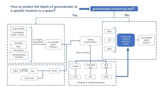
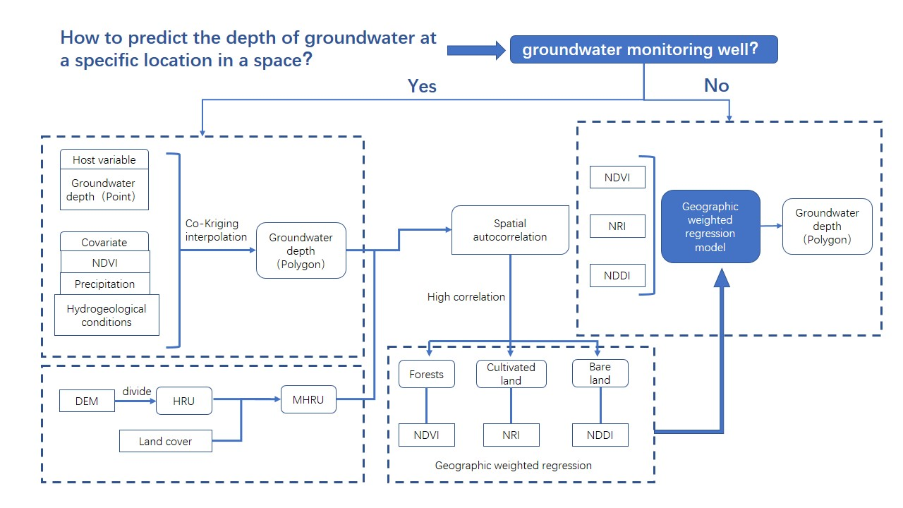
In our research, we focused on the spatial simulation of water depth. Since traditional groundwater depth monitoring uses monitoring wells to collect data, and groundwater is of great significance to human survival and life, it is necessary to obtain groundwater depth information at specific locations in space in today’s society. The groundwater system is unmonitored; therefore, we needed to study a model that can simulate the depth of groundwater in a certain area under specific conditions. In this study, two prediction models were set up to detect the presence or absence of local groundwater depth data. Based on the groundwater depth data of some points in the area, the cokriging interpolation model can be used to simulate the groundwater depth within the spatial range of the area. If there is no groundwater depth point data, the combination of remote sensing image bands can also simulate the distribution of groundwater to a certain extent. Effectively estimating the buried depth of groundwater in a specific area is of great significance for explaining the water cycle of the earth’s sphere and human development and utilization.

5. Conclusions

In this paper, we used the cokriging interpolation to calculate the groundwater depth data in the study area. At the same time, MHRU was divided by DEM and land coverage. Following this, spatial autocorrelation analysis was carried out using MHRU as the carrier, and the corresponding remote sensing inversion index was selected for geographically weighted regression. The main variables were groundwater depth in 2005, 2009, 2013, and 2017, and data that could spatially affect groundwater depth, such as NDVI, precipitation, and hydrogeological conditions, were used as covariates. The groundwater depth data are presented in space through collaborative kriging interpolation. In the four-year interpolation results, the groundwater depth data displayed little change on average, and the groundwater depth varies between 2 and 5 m.
The groundwater burial depth data after coordinated kriging interpolation was used to convert raster data into vector data spatially using the hydrological response unit model. Through hydrological analysis, the HRUs were demarcated and re-divided according to the land use type of the study area, which was the MHRU, totalling 551. Spatial autocorrelation analysis was carried out based on the assignment of the MHRU. In the four-year data, there were 135 high-value clusters and 114 low-value clusters. The overall groundwater burial depth shows aggregation characteristics, and the groundwater confluence process shows a gradually orderly state.
The overall analysis of the spatial–temporal differentiation characteristics of groundwater depth in the study area was then carried out. The groundwater has an obvious spatial differentiation pattern between the east and west, mainly from the land cover of the mountainous forest belt in the west and the farmland and dune belt in the east, as well as the difference in topography and landform. The groundwater table shows a trend of high in the west and low in the east. The average change of groundwater depth in the time series is not large but shows a gradual trend of accumulation, indicating the obstacles that hinder the recharge of groundwater are gradually being eliminated.
According to the accumulation characteristics through spatial autocorrelation analysis, the land cover type is associated with the accumulation characteristics of groundwater depth, and the characteristics of forest land, cultivated land, and bare land are prominent; therefore, a geographically weighted regression model of groundwater depth and NDVI, NDDI, and NRI was established and the spatial location information was combined. The NDVI representing the forest land and the adjusted R2 of the groundwater depth is 0.67. NRI representing the cultivated land and the adjusted R2 of the groundwater depth is 0.8675. NDDI representing the bare land and the adjusted R2 of the groundwater depth is 0.7875. The band index representing the land type has a good fitting effect with the groundwater burial depth, and the groundwater resources that cannot be directly monitored could be simulated and predicted by diversified land type characteristics; therefore, the development and utilization of groundwater resources in KAPZs should be combined with the above characteristics, rational planning, key development, and effective use. The effective use of groundwater can better maintain the stability of the water circulation system and provide better ecological service functions, which is of great significance for optimizing the ecological pattern of ECZ.

Author Contributions

Conceptualization, T.N. and J.Y.; methodology, T.N.; software, Q.Y.; validation, T.N. and D.Y.; formal analysis, Y.H.; investigation, S.L.; resources, X.M.; data curation, Q.L.; writing—original draft preparation, T.N.; writing—review and editing, T.N.; visualization, T.N.; supervision, D.Y.; project administration, D.Y.; funding acquisition, D.Y. All authors have read and agreed to the published version of the manuscript.

Funding

This research is supported by the National Key Research and Development Program of China (2016YFC0507303).

Acknowledgments

Thanks to the relevant department of Wengniute Banner for providing the data of groundwater monitoring wells over the years, so that we can complete this work. The authors also thank the reviewers for their valuable suggestions that helped to improve the quality of the manuscript.

Conflicts of Interest

The authors declare no conflict of interest.

Appendix A

Table A1. Groundwater depth monitoring well data.
Number2005200920132017AverageMaxMinElevationLongitudeLatitude
12.0782.8874.5892.9983.1384.5892.078642118.979242.91196
22.8652.9994.8652.4453.29354.8652.445635118.972642.9413
33.1253.4855.0042.7543.5925.0042.754636118.982442.96041
42.5872.6584.6892.8853.204754.6892.587635119.072142.96381
53.0042.7785.1143.0053.475255.1142.778620119.098642.933
62.7453.6585.5543.2513.8025.5542.745641119.095342.91452
73.1242.6353.5542.0412.83853.5542.041663118.957942.86041
83.212.9533.6752.5543.0983.6752.554684118.995942.74533
93.4583.7584.4413.3353.7484.4413.335668119.019342.72186
102.4252.5544.5872.5613.031754.5872.425760118.769642.83954
113.4252.8654.5213.7413.6384.5212.865618119.28142.88964
123.1473.9634.8953.6123.904254.8953.147617119.251742.81263
132.9452.5474.5212.7143.181754.5212.547657118.918542.64127
142.7412.5873.9872.8853.053.9872.587665118.896342.60969
152.9472.4944.1012.7743.0794.1012.494782118.714342.59284
163.0012.8643.2252.4142.8763.2252.414998118.348642.79786
173.8794.3415.7894.2564.566255.7893.8791385118.193642.78704
183.4574.1455.4244.7414.441755.4243.4571528118.117142.77843
192.5892.0141.4711.5521.90652.5891.471639118.935643.07449
202.8862.2261.4872.6542.313252.8861.487573119.022143.12981
212.5872.7841.8752.4192.416252.7841.875601119.001943.10315
223.7842.9942.7893.1973.1913.7842.789631118.698743.18637
233.1473.7972.7412.7783.115753.7972.741635118.646443.17077
244.8544.1127.0015.8415.4527.0014.112534119.331843.11926
253.6473.6954.3655.0144.180255.0143.647472119.402643.23153
263.1243.5213.1453.0583.2123.5213.058488119.348343.23171
272.4572.4712.7743.212.7283.212.457428119.669643.24446
282.7412.1142.0142.8742.435752.8742.014408119.783243.28839
293.8543.4823.4174.9783.932754.9783.417403119.857743.24789
303.0043.8544.1473.213.553754.1473.004385119.950443.30288
313.1473.6643.5643.6843.514753.6843.147380120.007243.32779
324.213.2454.5683.4473.86754.5683.245361120.104843.29964
333.2543.7894.683.6583.845254.683.254345120.203343.34744
342.4712.5413.2211.9952.5573.2211.995340120.306243.36716
353.2443.0153.9652.9943.30453.9652.994321120.393743.33634
363.7854.1744.6213.0243.9014.6213.024318120.480343.32451
373.4173.7843.6893.2543.5363.7843.254299120.583843.35076
382.112.0562.2541.5982.00452.2541.598291120.667243.38781
393.6583.6244.1023.6413.756254.1023.624310120.541243.3055
404.9955.8415.6695.6045.527255.8414.995315120.459343.21318
414.2515.3645.1075.1084.95755.3644.251312120.505143.24379
424.0254.8514.9525.114.73455.114.025310120.543643.25948
435.8415.1066.5215.6695.784256.5215.106352120.295843.10887
443.6693.5543.9643.0513.55953.9643.051338120.271943.00264
454.5513.9454.9574.1164.392254.9573.945415119.901343.02574
465.4714.8656.6656.3325.833256.6654.865722119.422842.94605
473.6543.1474.1023.1693.5184.1023.147439119.671342.81367
483.5473.6974.6573.6543.888754.6573.547452119.560642.75841
494.194.6144.1524.2514.301754.6144.152494119.503242.67225
503.6213.4873.9813.5473.6593.9813.487437119.614942.69795
513.2543.5974.5143.6423.751754.5143.254693119.022342.74746
523.1473.4173.6543.0673.321253.6543.067721118.850742.81537

References

  1. Peijun, A.; Zhang, Z.; Wang, L. Review of Earth Critical Zone Research. Adv. Earth Sci. 2016, 31, 1228–1234. [Google Scholar]
  2. Brantley, S.L.; Newark, N.S.F. Frontiers in exploration of the critical zone. In Proceedings of the Workshop on Frontiers in Exploration of the Critical Zone, Newark, NJ, USA, 24–26 October 2005. [Google Scholar]
  3. Lin, H.S. Earth’s Critical Zone and hydropedology: Concepts, characteristics, and advances. Hydrol. Earth Syst. Sci. Discuss. 2009, 6, 3417–3481. [Google Scholar] [CrossRef]
  4. Richter, D.D.; Megan, M.L. Environment monitoring earth’s critical zone. Science 2009, 326, 1067–1068. [Google Scholar] [CrossRef] [PubMed]
  5. Anderson, S.P.; Bales, R.C.; Duffy, C.J. Critical Zone Observatories: Building a network to advance interdisciplinary study of Earth surface processes. Miner. Mag. 2008, 72, 7–10. [Google Scholar] [CrossRef]
  6. Ahmadi, S.H.; Sedghamiz, A. Geostatistical Analysis of Spatial and Temporal Variations of Groundwater Level. Environ. Monit. Assess. 2006, 129, 277–294. [Google Scholar] [CrossRef] [PubMed]
  7. Zhang, H.; Wang, C.; Shanzhen, Y.; Jiang, Q. Geostatistical Analysis of Spatial and Temporal Variations of Groundwater Depth in Shule River. In Proceedings of the 2009 WASE International Conference on Information Engineering, Taiyuan, China, 10–11 July 2009. [Google Scholar]
  8. Alley, W.M.; Taylor, C.J. The Value of Long-Term Ground Water Level Monitoring. Ground Water 2001, 39, 801. [Google Scholar] [CrossRef] [PubMed]
  9. Kirk, C.; Philip, H. Using spatial models and Kriging techniques to optimize long-term ground-water monitoring networks: A case study. Environmetrics 2002, 5–6, 629–656. [Google Scholar]
  10. Desbarats, A.; Logan, C.; Hinton, M.J.; Sharpe, D. On the kriging of water table elevations using collateral information from a digital elevation model. J. Hydrol. 2002, 255, 25–38. [Google Scholar] [CrossRef]
  11. Kumar, S.; Sondhi, S.K.; Phogat, V. Network design for groundwater level monitoring in Upper Bari Doab Canal tract, Punjab, India. Irrig. Drain. 2005, 54, 431–442. [Google Scholar] [CrossRef]
  12. Banwart, S.A.; Chorver, J.; Gaillardet, G. Sustaining Earth’s Critical Zone Basic Science and Interdisciplinary Solutions for Global Challenges; The University of Sheffield: Sheffield, UK, 2013. [Google Scholar]
  13. Lee, B.; Hamm, S.-Y.; Jang, S.; Cheong, J.-Y.; Kim, G.-B. Relationship between groundwater and climate change in South Korea. Geosci. J. 2013, 18, 209–218. [Google Scholar] [CrossRef]
  14. Singh, S.K.; Singh, C.K.; Mukherjee, S. Impact of land-use and land-cover change on groundwater quality in the Lower Shiwalik hills: A remote sensing and GIS based approach. Open Geosci. 2010, 2, 124–131. [Google Scholar] [CrossRef]
  15. Danyar, S.; Yudong, S.; Jumakeld, M. Influence of groundwater level change on vegetation coverage and their spatial variation in arid regions. J. Geogr. Sci. 2004, 14, 323–329. [Google Scholar] [CrossRef]
  16. Fan, Y. Groundwater in the Earth’s critical zone: Relevance to large-scale patterns and processes. Water Resour. Res. 2015, 51, 3052–3069. [Google Scholar] [CrossRef]
  17. Jianfeng, Y.; Cuiguang, Z. Earth’s critical zone: A holistic framework for geo-environmental researches. Hydrogeol. Eng. Geol. 2014, 41, 98–104. [Google Scholar]
  18. Maxwell, R.M.; Kollet, S.J. Interdependence of groundwater dynamics and land-energy feedbacks under climate change. Nat. Geosci. 2008, 1, 665–669. [Google Scholar] [CrossRef]
  19. Chen, Y.X. The Study on the Development Model of Circular Economy in Agriculture and Animal Husbandry in Horqin Sandy Land. Master’s Thesis, Shanxi Normal University, Xi’an, China, 1 May 2014. (In Chinese). [Google Scholar]
  20. Gegentuya. The Study on Landscape Scale effect of Farming-Pastoral Zone with the Support of RS—Take Wengniute as the Example. Master’s Thesis, Inner Mongolia Normal University, Hohhot, China, 2010. (In Chinese). [Google Scholar]
  21. Xie, H.L.; Liu, L.M.; Li, B.; Zhang, X.S. Spatial Auto correlation Analysis of Multi-scale Land—Use Changes: A Case Study in Ongniud Banner, Inner Mongolia. Acta Geogr. Sin. 2006, 61, 389–400. (In Chinese) [Google Scholar]
  22. Tao, X.; Guang, H.; Huarui, H. County-scaled Change of Land Cover in Arid Region and Its Ecological Environmental Effects-A Case Study in Wengniute Banner, Inner Mongolia. Bull. Soil Water Conserv. 2016, 36, 240–246. [Google Scholar]
  23. Jiang, D.M.; Li, X.L.; Liu, Z.M. Ecological Footprint analysis of Horqin Sandy Land—A case study of Wengniuti Banner, Inner Mongilia. Arid Zone Res. 2004, 21, 263–268. (In Chinese) [Google Scholar]
  24. Kurylyk, B.L.; MacQuarrie, K.T.; McKenzie, J.M. Climate change impacts on groundwater and soil temperatures in cold and temperate regions: Implications, mathematical theory, and emerging simulation tools. Earth-Sci. Rev. 2014, 138, 313–334. [Google Scholar] [CrossRef]
  25. Yumi, I.; Kimihito, N.; Haruhiko, H.; Shigeto, K. Assessment of factors influencing groundwater-level change using groundwater flow simulation, considering vertical infiltration from rice-planted and crop-rotated paddy fields in Japan. Hydrogeol. J. 2014, 22, 1841–1855. [Google Scholar]
  26. Moeck, C.; Brunner, P.; Hunkeler, D. The influence of model structure on groundwater recharge rates in climate-change impact studies. Hydrogeol. J. 2016, 24, 1171–1184. [Google Scholar] [CrossRef] [Green Version]
  27. Michelle, M.; James, F. Downscaling grace remote sensing datasets to high-resolution groundwater storage change maps of california’s central valley. Remote Sens. 2018, 10, 143. [Google Scholar] [CrossRef] [Green Version]
  28. Kotowski, T.; Satora, S. Analysis of the spatial variability of the concentrations of Na+ and K+ ions in the groundwater sourced in Southern Poland. Environ. Prot. Eng. 2016, 42, 5–18. [Google Scholar] [CrossRef]
  29. Zhang, Z.; Cheng, Q. GIS spatial statistical analysis of groundwater in GTA, Canada. In Proceedings of the International Conference on Image Processing, Catalonia, Spain, 14–18 September 2003; Volume 4. [Google Scholar]
  30. Desbarats, A.J.; Hinton, M.J.; Logan, C.E.; Sharpe, D.R. Geostatistical mapping of leakance in a regional aquitard, Oak Ridges Moraine area, Ontario, Canada. Hydrogeol. J. 2001, 9, 79–96. [Google Scholar] [CrossRef]
  31. ASCE Task Committee on Geostatistical Techniques in Geohydrology of the Ground Water Hydrology Committee of the ASCE Hydraulics Division. Review of geostatistics in geohydrology 1: Basic concepts 2: Applications. ASCE J. Hydraul. Eng. 1990, 116, 612–658. [Google Scholar] [CrossRef]
  32. Rahmati, O.; Melesse, A.M. Application of Dempster–Shafer theory, spatial analysis and remote sensing for groundwater potentiality and nitrate pollution analysis in the semi-arid region of Khuzestan, Iran. Sci. Total. Environ. 2016, 568, 1110–1123. [Google Scholar] [CrossRef]
  33. Al-Ruzouq, R.I.; Shanableh, A.; Merabtene, T.; Siddique, M.; Khalil, M.A.; Idris, A.; Almulla, E. Potential groundwater zone mapping based on geo-hydrological considerations and multi-criteria spatial analysis: North UAE. Catena 2019, 173, 511–524. [Google Scholar] [CrossRef]
  34. Salman, A.; Al-Qinna, M.; Kuisi, M.A. Spatial analysis of soil and shallow groundwater physicochemical parameters in El-Mujib Basin-central Jordan. J. Asian Earth Ences 2014, 79 Pt A, 366–381. [Google Scholar] [CrossRef]
  35. Gleeson, T.; Befus, K.M.; Jasechko, S.; Luijendijk, E.; Cardenas, M.B. The global volume and distribution of modern groundwater. Nat. Geosci. 2015, 9, 161–167. [Google Scholar] [CrossRef]
  36. Wang, H.M.; Luo, Y.M.; Jiang, D.M. Unsymmetrical variation of the maximum and minimum air temperatures in Wengniute Banner, Horqin Sand Land. Arid Zone Res. 2007, 2, 261–267. (In Chinese) [Google Scholar]
  37. Benli, L.; Wei, Z. Changes in Climatic Factors and Dune Activity Index at Ongniud Banner During 1957–2014. Bull. Soil Water Conserv. 2017, 37, 270–273, discussion 280. [Google Scholar]
  38. Wen-Han, C.; Qiang, Z.; Xiao-Qin, L.; Xiao, S.; Hong-Ye, L.I.; Laboratory, N.K. Estimation nitrate of concentration in drinking water based on cooperative Kriging, interpolation. China Rural Water Hydropower 2018, 6, 84–87. [Google Scholar]
  39. Xu, C.; Zeng, W.; Huang, J.; Wu, J. Modelling soil water content in plow layer using co-Kriging interpolation based on hyperspectral data. Nongye Gongcheng Xuebao Trans. Chin. Soc. Agric. Eng. 2014, 30, 94–103. [Google Scholar]
  40. Knotters, M.; Brus, D.; Voshaar, J.O. A comparison of kriging, co-kriging and kriging combined with regression for spatial interpolation of horizon depth with censored observations. Geoderma 1995, 67, 227–246. [Google Scholar] [CrossRef]
  41. Park, J.; Jang, D.-H. Application of MK-PRISM for interpolation of wind speed and comparison with co-kriging in South Korea. GIScience Remote Sens. 2016, 53, 421–443. [Google Scholar] [CrossRef]
  42. Song, Q.-L.; Du, D.-W.; Ding, M.; Yan, S.-J. Application of Co-Kriging Method to Interpolation of Surface Temperature Data in East China Sea. Coast. Eng. 2011, 30, 49–55. [Google Scholar]
  43. Teng, N.; Depeng, Y.; Qian, L.; Qiang, Y.; Jiaxin, Y.; Minzhe, F. Research on Ground Deformation Based on GLM-PSO-coKriging Model. Geo-Inf. Sci. 2018, 20, 1579–1591. [Google Scholar]
  44. Koziel, S.; Couckuyt, I.; Ogurtsov, S.; Dhaene, T. Cost-efficient electromagnetic-simulation-driven antenna design using co-Kriging. IET Microw. Antennas Propag. 2012, 6, 1521–1528. [Google Scholar] [CrossRef] [Green Version]
  45. Smedema, L.K.; Shiati, K. Irrigation and Salinity: A Perspective Review of the Salinity Hazards of Irrigation Development in the Arid Zone. Irrig. Drain. Syst. 2002, 16, 161–174. [Google Scholar] [CrossRef]
  46. Sophocleous, M.; Paschetto, J.E.; Olea, R.A. Ground-Water Network Design for Northwest Kansas, Using the Theory of Regionalized Variables. Ground Water 1982, 20, 48–58. [Google Scholar] [CrossRef]
  47. Xu, Z.; Weiguo, J.; Tinggang, Z.; Hong, T. Hydrological Response Unit Division for Dongting Lake Based on DEM and GIS. Geogr. Geo-Inf. Sci. 2009, 25, 17–21. [Google Scholar]
  48. Kumar, S.; Mishra, A. Critical Erosion Area Identification Based on Hydrological Response Unit Level for Effective Sedimentation Control in a River Basin. Water Resour. Manag. 2015, 29, 1749–1765. [Google Scholar] [CrossRef]
  49. Yulianur, A.; Rizalihadi, M.; Bachtiar, S. Hydrological Response Unit Analysis Using AVSWAT 2000 for Keuliling Reservoir Watershed, Aceh Province, Indonesia. Aceh Int. J. Sci. Technol. 2015, 4, 32–40. [Google Scholar] [CrossRef] [Green Version]
  50. Macdonald, M.K.; Pomeroy, J.W.; Pietroniro, A. Hydrological response unit-based blowing snow modelling over an alpine ridge. Hydrol. Earth Syst. Sci. Discuss. 2010, 7, 1167–1208. [Google Scholar] [CrossRef] [Green Version]
  51. Aytaç, E. Unsupervised learning approach in defining the similarity of catchments: Hydrological response unit based k-means clustering, a demonstration on Western Black Sea Region of Turkey. Int. Soil Water Conserv. Res. 2020, 8, 321–331. [Google Scholar] [CrossRef]
  52. Chifflard, P.; Moulding, D.; Petri, J.T.; Zemke, J.J.; Reiss, M. Surface runoff of horse grazed pasture—A disregarded hydrological response unit in low mountain ranges. DIE ERDE–J. Geogr. Soc. Berl. 2018, 149, 76–85. [Google Scholar]
  53. Xin, Z.; Qiyu, L.; Xinyong, C. Development of a location-weighted landscape contrast index based on the minimum hydrological response unit. J. Oceanol. Limnol. 2018, 36, 1236–1243. [Google Scholar]
  54. Wei, Z.; Zhang, B.; Liu, Y.; Xu, D. The Application of a Modified Version of the SWAT Model at the Daily Temporal Scale and the Hydrological Response unit Spatial Scale: A Case Study Covering an Irrigation District in the Hei River Basin. Water 2018, 10, 1064. [Google Scholar] [CrossRef] [Green Version]
  55. Fang, C.; Sun, S.; Jia, S.; Li, Y. Groundwater Level Analysis Using Regional Kendall Test for Trend with Spatial Autocorrelation. Ground Water 2018, 57, 320–328. [Google Scholar] [CrossRef]
  56. Liu, Y.; Lan, S.-S.; Zhang, Y.-X.; Li, F.-C.; Hou, S.-K. Spatio-temporal Evolution of Groundwater Vulnerability Based on Spatial Autocorrelation. Huan Jing ke Xue = Huanjing Kexue 2017, 38, 4236–4244. [Google Scholar]
  57. Lichstein, J.W.; Simons, T.R.; Franzreb, S.K.E. Spatial Autocorrelation and Autoregressive Models in Ecology. Ecol. Monogr. 2002, 72, 445–463. [Google Scholar] [CrossRef]
  58. Bini, L.M.; Hawkins, B.A. Spatial autocorrelation and red herrings in geographical ecology. Glob. Ecol. Biogeogr. 2003, 12, 53–64. [Google Scholar] [CrossRef] [Green Version]
  59. Kissling, W.D.; Carl, G. Spatial autocorrelation and the selection of simultaneous autoregressive models. Glob. Ecol. Biogeogr. 2007, 17, 59–71. [Google Scholar] [CrossRef]
  60. Fan, C.; Myint, S. A comparison of spatial autocorrelation indices and landscape metrics in measuring urban landscape fragmentation. Landsc. Urban Plan. 2014, 121, 117–128. [Google Scholar] [CrossRef]
  61. Tao, L.; Cao, Y.H. Construction of spatial autocorrelation method of spatial-temporal proximity and its application: Taking regional economic disparity in the Yangtze River Delta as a case study. Geogr. Res. 2010, 29, 351–360. [Google Scholar]
  62. Mihai, V.; Bart, K. Spatial autocorrelation: An overlooked concept in behavioral ecology. Behav. Ecol. 2020, 21, 902–905. [Google Scholar]
  63. Václavík, T.; Kupfer, J.A.; Meentemeyer, R.K. Accounting for multi-scale spatial autocorrelation improves performance of invasive species distribution modelling (iSDM). J. Biogeogr. 2011, 39, 42–55. [Google Scholar] [CrossRef]
  64. Bahn, V.; O’Connor, R.J.; Krohn, W.B. Importance of spatial autocorrelation in modeling bird distributions at a continental scale. Ecography 2006, 29, 835–844. [Google Scholar] [CrossRef]
  65. Fotheringham, A.S.; Crespo, R.; Yao, J. Geographical and Temporal Weighted Regression (GTWR). Geogr. Anal. 2015, 47, 431–452. [Google Scholar] [CrossRef] [Green Version]
  66. Mas, J.-F.; Cuevas, G. Local Deforestation Patterns in Mexico—An Approach using Geographiccally Weighted Regression. In Proceedings of the 1st International Conference on Geographical Information Systems Theory, Applications and Management, Barcelona, Spain, 28–30 April 2015; pp. 54–60. [Google Scholar]
  67. Yu, H.; Gong, H.; Chen, B.; Liu, K.; Gao, M. Analysis of the influence of groundwater on land subsidence in Beijing based on the geographical weighted regression (GWR) model. Sci. Total. Environ. 2020, 738, 139405. [Google Scholar] [CrossRef]
  68. Shang, R.-K.; Shiu, Y.-S.; Ma, K.-C. Using geographically weighted regression to explore the spatially varying relationship between land subsidence and groundwater level variations: A case study in the Choshuichi alluvial fan, Taiwan. In Proceedings of the 2011 IEEE International Conference on Spatial Data Mining and Geographical Knowledge Services, Fuzhou, China, 29 June–1 July 2011; pp. 21–25. [Google Scholar]
  69. Yueming, L.U.; Liang, W.; Agen, Q.; Yongchuan, Z.; Yangyang, Z. A Temporal-Spatial Geographic Weighted Regression Method Based on Principal Component Analysis. J. Geomat. Sci. Technol. 2017, 6, 654–658. [Google Scholar]
  70. Littidej, P.; Buasri, N. Built-Up Growth Impacts on Digital Elevation Model and Flood Risk Susceptibility Prediction in Muaeng District, Nakhon Ratchasima (Thailand). Water 2019, 11, 1496. [Google Scholar] [CrossRef] [Green Version]
  71. Seyed, H.A.; Abbas, S. Application and Evaluation of Kriging and Co-Kriging Methods on Groundwater Depth Mapping. Environ. Monit. Assess. 2008, 138, 357–368. [Google Scholar]
  72. Zhang, Y.; Chiew, F.H.S.; Li, M.; Post, D.A. Predicting Runoff Signatures Using Regression and Hydrological Modeling Approaches. Water Resour. Res. 2018, 54, 7859–7878. [Google Scholar] [CrossRef]
  73. Dong, Y.; Jiang, C.; Suri, M.R.; Pee, D.; Meng, L.; Goldstein, R.E.R. Groundwater level changes with a focus on agricultural areas in the Mid-Atlantic region of the United States, 2002–2016. Environ. Res. 2019, 171, 193–203. [Google Scholar] [CrossRef] [PubMed]
  74. Scanlon, B.R.; Healy, R.; Cook, P. Choosing appropriate techniques for quantifying groundwater recharge. Hydrogeol. J. 2002, 10, 347. [Google Scholar] [CrossRef]
  75. Javi, S.T.; Malekmohammadi, B.; Mokhtari, H. Application of geographically weighted regression model to analysis of spatiotemporal varying relationships between groundwater quantity and land use changes (case study: Khanmirza Plain, Iran). Environ. Monit. Assess. 2014, 186, 3123–3138. [Google Scholar] [CrossRef] [PubMed]
  76. Ma, T.-S.; Sophocleous, M.; Yu, Y.-S. Geostatistical Applications in Ground-Water Modeling in South-Central Kansas. J. Hydrol. Eng. 1999, 4, 57–64. [Google Scholar] [CrossRef]
  77. Nunes, L.M.; Cunha, M.; Ribeiro, L. Groundwater Monitoring Network Optimization with Redundancy Reduction. J. Water Resour Plan. Manag. 2004, 130, 33–43. [Google Scholar] [CrossRef] [Green Version]
Figure 1. Distribution of the study area and groundwater station.
Applsci 10 07105 g001
Figure 2. Seasonal changes in groundwater depth.
Applsci 10 07105 g002
Figure 3. Processing flow chart.
Applsci 10 07105 g003
Figure 4. Distribution map of training sample points.
Applsci 10 07105 g004
Figure 5. Ordinary kriging interpolation result in (a) 2005, (b) 2009, (c) 2013, (d) 2017.
Applsci 10 07105 g005
Figure 6. Cokriging interpolation result in (a) 2005, (b) 2009, (c) 2013, (d) 2017.
Applsci 10 07105 g006
Figure 7. Hydrological response unit distribution map.
Applsci 10 07105 g007
Figure 8. Distribution of the minimum response unit.
Applsci 10 07105 g008
Figure 9. Autocorrelation characteristics of groundwater depth.
Applsci 10 07105 g009
Figure 10. Net relatedness index (NRI) geographic weighted regression standardized residuals.
Applsci 10 07105 g010
Figure 11. Normalized difference vegetation index (NDVI) geographic weighted regression standardized residuals.
Applsci 10 07105 g011
Figure 12. Normalized difference drought index (NDDI) geographic weighted regression standardized residuals.
Applsci 10 07105 g012
Table 1. The 2005, 2009, 2013, and 2017 groundwater information.
YearsAverageMaxMin
20053.3915.8412.078
20093.4355.8412.014
20134.1797.0011.471
20173.4496.3321.552
Table 2. Interpolation accuracy evaluation of different semivariogram models.
Mean ErrorRoot Mean Square ErrorMean Standard ErrorStandardized Average ErrorNuggetRangeSill
Stable model0.4170.4250.2361.0650.0242821677.324
Ring model0.5981.3520.5241.6540.0341231216.895
Spherical model0.8890.5780.6342.0060.183950837.119
Three-ball model0.6470.6941.0321.4170.0964748988.886
Five-ball model1.0571.1520.5591.3620.129941528.912
Index model1.1150.8930.4870.9970.115468937.912
Gaussian model0.7840.7410.9641.0740.0734132117.112
Rational quadratic model0.9651.520.8351.2540.0998534216.789
J-Bessel model1.3210.6651.231.3670.123149766.661
K-Bessel model−0.9630.7831.0081.6340.0976323417.731
Hole model0.7421.0050.6412.1040.0671222837.901
Table 3. Model partition accuracy evaluation.
Number2005200920052005
ActualOrdinaryCokrigingActualOrdinaryCokrigingActualOrdinaryCokrigingActualOrdinaryCokriging
East12.5783.4432.9092.8933.3212.4232.8863.8873.2122.7983.3212.894
23.1123.3323.3543.3393.9973.4123.3213.3393.0912.9953.3393.521
53.0982.7782.8982.9972.8973.1193.7123.0123.4453.2133.6813.102
Central33.7643.2133.6753.9083.1173.8713.9653.1213.6653.5893.1913.612
42.9973.6643.3983.7762.9873.8793.1213.9853.9963.3023.4412.891
74.0073.5533.6784.1124.3213.8883.8733.1173.2113.9953.3374.203
West63.5123.3793.2883.6122.6783.3813.7793.1233.3393.4782.8953.546
83.6413.3543.5623.9783.6933.3373.3123.7852.9083.3573.0213.555
93.1622.8863.1124.1193.2783.9032.9972.7753.0193.4123.0043.336
102.9983.3393.0952.8953.8712.6693.1093.8613.7973.1123.6583.389
Table 4. Net relatedness index (NRI) geographic weighted regression fitting parameters.
YearAICcR2R2 Adjusted
2005−86.140.91190.8756
2009−43.060.91850.8890
2013−484.00.97040.9586
2017−61.830.81990.7543
Table 5. Normalized difference vegetation index (NDVI) geographic weighted regression fitting parameters.
YearAICcR2R2 Adjusted
2005−48.690.83250.7889
2009−30.980.60410.4918
2013−99.590.79580.7387
2017−41.390.74220.6698
Table 6. Normalized difference drought index (NDDI) geographic weighted regression fitting parameters.
YearAICcR2R2 Adjusted
2005−143.70.81530.7766
2009−44.380.83180.7823
2013−282.20.93980.9170
2017−54.830.72670.6805

