Abstract
The residue number system (RNS) is widely used for data processing. However, division in the RNS is a rather complicated arithmetic operation, since it requires expensive and complex operators at each iteration, which requires a lot of hardware and time. In this paper, we propose a new modular division algorithm based on the Chinese remainder theorem (CRT) with fractional numbers, which allows using only one shift operation by one digit and subtraction in each iteration of the RNS division. The proposed approach makes it possible to replace such expensive operations as reverse conversion based on CRT, mixed radix conversion, and base extension by subtraction. Besides, we optimized the operation of determining the most significant bit of divider with a single shift operation of the modular divider. The proposed enhancements make the algorithm simpler and faster in comparison with currently known algorithms. The experimental simulation using Kintex-7 showed that the proposed method is up to 7.6 times faster than the CRT-based approach and is up to 10.1 times faster than the mixed radix conversion approach.
1. Introduction
The residue number system (RNS) has attracted many researchers as a basis for computing, and the interest taken in it has increased dramatically over the latest decade, which could be seen from the large number of papers focusing on the practical application of RNS in digital signal processing, image processing systems, cryptographic systems, quantum automated machines, neural computers systems, massive concurrency of operations, cloud computing, etc. [1,2,3,4,5,6,7].
RNS, if compared to other scales of notation, offers the advantage of rapid addition and multiplication, which causes stirs of interest in the RNS in areas requiring large amounts of computation. However, some operations, such as comparison and division of numbers, are very complicated in the RNS. Finding faster division algorithms would allow detecting more promising new areas to apply RNS.
The known RNS division algorithms [8,9,10,11,12,13,14,15,16,17,18,19,20,21,22,23] can be divided into two classes: based on the comparison of numbers, and based on the subtraction.
The algorithm for integer division operates similarly to a conventional binary division proposed in [1,2]. This algorithm and its modifications have a major drawback, namely that each iteration requires a comparison of numbers.
The algorithm without these drawbacks, as proposed in [1,2], is based on replacing the divider by an approximate value, which may be the product of one or several RNS modules. The algorithm provides a correct result for the condition , where b is an actual divider and is an approximation of b. It is easy to see that this condition cannot be satisfied for all moduli sets (for example: p1 = 9, p2 = 11, b = 4).
The main disadvantages of this algorithm are the necessity of mixed radix conversion (MRC) and scaling operations use, and special logic and tables for determining the approximate divider. There have been proposed several algorithms for solving the problem of division based on a comparison of numbers and methods of determining the sign, which can be classified as follows: [8,10,15] using MRC, [9] to formulate the problem in terms of determining the even numbers, and [11] using the base extension operation in iterations. All the proposed algorithms, however, have the disadvantage of long computation time and high hardware costs due to the use of MRC, Chinese remainder theorem (CRT), and other costly operations.
In [12,13,14,16], a high-speed division algorithm is presented, which uses the comparison of higher degrees of dividend and divisor instead of using the MRC and CRT for the division of modular numbers. The time complexity and hardware costs in these algorithms are smaller than other algorithms, although this algorithm contains redundant stages. To speed up the calculation of the current quotients, Hung and Parhami suggested a division algorithm based on parity checking, in which the quotient calculation occurs two times faster than the algorithms [14,16]. However, the calculation of the higher powers of two is time-consuming in the RNS, which are carried out in each cycle.
The known algorithm of division in the RNS format, in addition to the RNS moduli set, also uses a replacement module system, which is an auxiliary to preserve the dividend and divisor residues. Presented in the RNS dividend and divisor are converted into a variety of RNS presentations with the various modules of the system [18]. Using two moduli sets of RNS leads to a large redundancy and the necessity for direct and reverse conversion from moduli set to the auxiliary and back for the division operation, which drastically reduces its speed. A fast algorithm for the division based on the use of the index over the Galois field transformation GF(p) is proposed in [18], which was simply implemented using LUTs (Look-Up Table). However, this algorithm is effective when processing data no more than 6–10 bits and when a modulus is a prime number. Thus, this algorithm is not efficient for large RNS ranges.
Most of the known iterative algorithms contain a large number of operations in each iteration. According to the authors, the algorithm based on the CRT with fractions considered in [11,17,23] is the best and has the time complexity O(nb), where n is the number of RNS modules and b is the number of bits in each module, assuming that the value of each module is more or less the same. The disadvantage of this algorithm is a set of operations performed in each iteration: the operations of addition, multiplication, comparison, and parity checking. Furthermore, the execution of the algorithm requires the conversion of the quotient from the system {−1, 0, 1} into the system {0, 1}, which gives an additional burden on the runtime of a modular division of number procedures.
In this paper, we propose an algorithm for division in the general case in the RNS using only the register shifts and summations. The improved algorithm has the following properties: it is very fast compared to the algorithms that are still available; has no restrictions on the dividend and divisor (except for when the divisor is equal to zero); it does not use a preliminary estimate of the coefficient; it does not use the back divisor; and does not use the base expansion operation. In [20], a similar approach based on mixed radix number system (MRNS) is proposed; however, in addition to the original RNS moduli set, it also used an auxiliary modulus set, which requires additional calculations for data conversion and significantly slows down the calculation of the division result. The proposed algorithm allows increasing the performance of the division algorithm by using the CRTf method. In [14,16] the idea of the most significant bits for a quotient was proposed for an RNS with special moduli sets and , while in the proposed work, this approach is expanded to the case of general moduli set.
The main difference between this paper and [22] is that in this paper, a division algorithm for redundant RNS is proposed. Redundant RNS is intended for the organization of fault-tolerant calculations, while its modules are separated into informational, by which information is encoded, and redundant, necessary to restore information in case of errors. Separation of modules into information and redundant allows simplifying calculations by taking into account the information and redundant range of the system.
The known algorithms for dividing the numbers represented in the RNS are based on the absolute values of the dividend and the divisor. In this paper, we do not use the absolute values but their relative values, which allows reducing the computational complexity of division algorithms.
The rest of the paper is organized as follows: Section 2 describes the basics of RNS (Section 2.1) and approximate method for determining the placement of the number in it (Section 2.2). The proposed RNS division algorithm is presented in Section 2.3. Results and discussion are presented in Section 3.
2. An Approximate Method for Determining the Positional Feature of the Modular Number
2.1. Residue Number System
In the RNS, a positive integer is represented as a bank of residues to selected co-prime bases. This approach allows one to replace operations with large numbers by operations with small numbers, which are represented as residues of the division of large numbers by earlier selected relatively prime modules . Let
Then, an integer A can be associated with the set of the least non-negative residues over one of the corresponding numbers. This correspondence will be one-to-one until , according to the CRT. The set can be considered as one of the methods of the representation of the integer A in a computer, i.e., the modular representation or representation in the RNS.
The main advantage of this representation is the fact that the addition, subtraction, and multiplication operations are implemented very simply by the formulas:
These operations are called modular, since, for their execution in the RNS, it is sufficient to fulfill one cycle of processing numerical values. In addition, this processing occurs in parallel, and the information value in each modulo channel does not depend on the other modulo channels.
Thus, there are three main advantages of RNS [1].
- There is no carry propagation between RNS arithmetic units. Large numbers represented in the form of small residues that leads to faster data processing.
- When using the RNS, large numbers are encoded into a set of small residues, which reduces the complexity of the arithmetic units and simplifies the computing system.
- RNS is a non-positional system with independent arithmetic units; therefore, an error in one channel does not apply to others. Thus, the processes of error detection and error correction are simplified.
However, such operations as sign detection, comparison, division, and some others are time-consuming and expensive in the RNS [4].
2.2. Approximate Method
An analysis of difficult (non-modular) operations has shown that they can be represented exactly or approximately, so the methods for calculating positional characteristics can be divided into two groups:
- –
- Methods for accurate calculation of positional characteristics.
- –
- Methods for the approximate calculation of positional characteristics.
The methods for accurate calculation of positional characteristics are discussed in [1,2,3]. In this paper, we investigate the approximate method for calculating positional characteristics that can significantly reduce the hardware and time costs due to operations performed on positional codes of reduced capacity. In this regard, there is an issue of using the approximate method when calculating a certain number of non-modular procedures: determining intervals of numbers; number sign; number comparison, in cases where there is no need to know the exact value; and the difference between the numbers.
The point of the approximate method for calculating the positional characteristics of modular number is based on employing the relative values of the analyzed numbers to the full range defined by the CRT, which connects the positional number a with its representation in the remainder , where αi is the smallest non-negative residues of the number in relation to the modules of the residue number system with the following expression:
where pi are RNS modules, is the range of RNS, , and is a multiplicative inversion of Pi modulo pi.
If we divide the left and right parts of Expression (4) by the constant P, corresponding to the range of numbers, we will get the approximate value
where denotes the fraction of (or Modulo 1 operation) [24], are constants of the chosen system, and αi are positions of the number represented in the RNS in modules pi, where , and the value of the Expression (5) will be in the range [0, 1). The result of the sum shall be found after summation and discarding the integer part while maintaining the fractional part of the sum. The fractional value contains information both on the magnitude of the number and on its sign. If , then the number a is positive and F(a) is equal to the number of a, divided by P. Otherwise, a is a negative number, and 1 − F(a) indicates a relative value. Rounding F(a) to 2−t bits will be denoted as . The exact value of F(a) is determined by inequalities . The integer part, obtained through summing the constants ki, is a rank number; that is, a non-positional feature that shows how many times the range of the system P was surpassed while passing from the number representation in the residue number system to its positional representation. If necessary, the rank can be determined directly through the operation of the summation the constants ki. The fractional part can also be written as because . The number of positions in the fractional part of the number is determined by the maximum potential difference between the adjacent numbers. In case of accurate comparison, which is widely used in the division of numbers, you need to calculate a value that is equivalent to the conversion of the RNS into the positional notation.
Rounding the F(a) value will inevitably result in an error. Let us denote . Work [22] shows that it is necessary to use bits after the decimal point when rounding the value F(a), so that the resulting error has no effect on the accuracy of calculations. In other words, there is established a one-to-one correspondence between the set of numbers represented in the RNS and the plurality of values. Using the variables in calculations, in terms of algorithmic complexity, is equivalent to applying the inverse transformation from the RNS into the positional notation using the CRT. This method is slow and therefore, in practice, the use of calculations with the values is not rational. In [22], it is shown that it is possible to use the values , where , for operations of determining the number sign in the RNS. The point of this approach is based on the fact that when determining the sign there is no need to know the exact value of the number, and it is just enough to know about the range within which the number tested falls.
The algorithm for determining the sign of the number serves the basis for number comparison algorithms. Determining the sign of the number in the RNS using the values , takes the following operations:
- «Rough estimate». At this stage, the value , is used. If , then the number a is positive. If , then the number is negative.
- «Clarification». If the number a falls into none of the intervals as indicated in Step 1, then a rechecking of the number is needed with maximum precision calculation regarding the values. If , then the number a is positive. If , then the number a is negative.
The speed of the algorithm at the stage of the «rough estimate» depends on how little the value is compared to N. However, if is taken as too little, then the intervals in Step 1 may be so small that the algorithm for numerous numbers in the RNS would require the use of the «clarification» stage, while the benefit of using a small capacity at the «rough estimate» stage would be dismissed completely. For example, in [13], it is proposed to use the case when that is usually too small for practice. Instead, we suggest using an estimation from [22], which shows that the optimal speed of the algorithm is achieved with . Here below comes a comparison of the and N capacities for the RNS, where the ranges of 16, 32, and 64 bits are implemented.
1. Sixteen bits. RNS modules 7, 17, 19, 29.
2. Thirty-two bits. RNS modules 2, 3, 5, 11, 13, 19, 23, 29, 79.
3. Sixty-four bits. RNS modules 2, 11, 17, 19, 23, 31, 41, 53, 59, 61, 71, 79, 83.
Thus, with an RNS of a 16-bit range, the «rough estimate» is done using the values with a capacity of bits, while the «clarification» takes place at the N = 23 bit precision. The speed of the rough estimate goes up by 2.09 times. For an RNS with a 32-bit range, the «rough estimate» employs a capacity of bits, while the «clarification» requires N = 40 bits for calculation. The speed of the rough estimate increases 3.08 times. For a 64-bit RNS, the «rough estimate» would use a capacity of bits, while the «clarification» requires N = 74 bits. The speed of the rough estimate increases 4.62 times. These results show that, for large ranges, the capacity employed for the rough estimate is significantly lower than the accurate calculation capacity N, which allows significant gains in terms of speed when performing non-modular operations.
Figure 1 shows the location of the mentioned intervals for positive and negative numbers in the RNS, and the location of the ambiguity areas, where it is possible to wrongly determine the sign. For the redundant RNS, the numerical range shows a redundancy zone. This allows reducing the number of the checked conditions due to the fact that the sets of the admissible positive numbers and the areas of the erroneous sign determination would no longer intersect (Figure 2). Thus, when speaking of a redundant RNS, determining the sign is reduced to the following tasks.
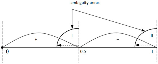
Figure 1.
Position of ambiguity areas when determining the sign and the intervals for positive and negative numbers for irredundant residue number system (RNS).
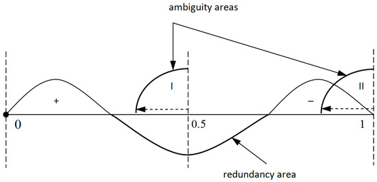
Figure 2.
Position of ambiguity areas when determining the sign and the intervals for positive and negative numbers for redundant RNS.
- «Rough estimate». If , then the number a is positive. If , then the number a is negative.
- «Clarification». If the number a is not included in any of the intervals in Step 1, then there is a sign rechecking needed using the variables. If , then the number a is positive. If , then the number a is negative.
Let us have a view on employing the approximate method by comparing the numbers in the RNS.
Example 1.
We have a system of bases,,,.
Then,,,,,.
The constants ki used for computing the relative values are:
For precise operations with relative sizes of numbers in the RNS, it is necessary to use characters after the decimal point. For a quick «rough estimate», we will use decimals. The constants ki rounded up to 7 and 12 bits after the decimal point, are, respectively:
Seven bits: k1 = 0.1000000; ; ; ;
Twelve bits: ; ; ; .
The «rough estimate» takes checking the conditions and (Step 1 of the algorithm), which in the binary form will appear as
1.1. If , then the number a is positive.
1.2. If , then the number a is negative.
Let us compare the two numbers a = 97 и b = 8 presented in the RNS on the bases , , , and . Let us define the numbers a and b in the RNS as: a = (1, 1, 2, 6), b = (0, 2, 3, 1). The difference is a − b = (1, 1, 2, 6) − (0, 2, 3, 1) = (1, 2, 4, 5). We will also define the sign a − b. For the «rough estimate», we will find that . The values found meets the condition of Step 1 of the algorithm, that is 0 < 0.0110001 < 0.0110011, so we can conclude that a – b > 0, which produces a > b.
Now, let us compare the two numbers a = 97 and b = 96 as presented in the RNS on the bases , , , and . Now, we will define the numbers a and b in the RNS: a = (1, 1, 2, 6), b = (0, 0, 1, 5). The difference is a − b = (1, 1, 2, 6) – (0, 0, 1, 5) = (1, 1, 1, 1). We will define the sign a − b. For the «rough estimate», . None of the conditions are met regarding the value obtained, so it will take a clarification stage of the algorithm. For the «accurate estimation», we will find . This value follows the condition of Step 2 of the algorithm, so we conclude that a – b > 0, where a > b.
The example above serves an illustration of employing the approximate method for computing in the RNS. It has been shown how to take into account the error that occurs when using a small . In practice, for most cases, it would be enough to carry out a «rough estimate», a run wherein it takes operating with numbers whose capacity is close to the logarithm of the full range capacity. Therefore, the complexity of the «rough estimate» is committed to , while the complexity of the «clarification» stage tends to O(n).
2.3. Division Algorithm in the RNS
The algorithm for the integer division could be described with an iterative scheme, which is performed in two stages. The first stage implies a search for the highest power 2i when approximating the quotient with a binary sequence. The second stage involves clarification of the approximating series. To get a range greater than P, you can select a value ; thus, it will take expanding the RNS base through adding an extra module. To avoid this base expansion, which is a computationally complex operation, we need to compare not the dividend with the interim divisors but the current results of the iteration (i) with the values of the previous iterations (i − 1). We will repeat the process of doubling the divider as long as the intermediate divider at the i iteration is below that of the i − 1 iteration. This would allow meeting the condition .
The division algorithm can be described with the following rules.
A certain rule φ is constructed, which, for each pair of positive integers, a and b will assign a certain positive number qi, where i is the number of the iteration, so that , i.e., . Then, the division of a by b will follow the rule: based on the operation φ, each pair of a and b will be assigned a corresponding number , so that , i.e., . We will take the values 2i as and place them into the memory as the constants . Given that, the i + 1 operation does not depend on the i-th operation, which allows performing iterations in parallel. Furthermore, in each iteration, there are only two operations performed: multiplication of the constant divisor by 2i, and comparison of the obtained values with the dividend.
If , then the division is complete; if , then following the rule φ, the pair of numbers will get a q2 assigned, so that , i.e., . If , then the division is completed, and if , then following the rule φ, the pair of numbers is assigned a q3, so that , etc. Since the consistent application of the operation φ leads to a decreasing sequence of integers , then the algorithm is implemented in a finite number of steps. Let us assume that at step m there is a case 0 < bqm recorded, which means the end of the division operation. Then, we finally obtain , where the sequence is the approximation of the quotient, which may contain some extra qi. Next, we need clarification for the resulting approximating series. In [14] and [16], the idea of the most significant bits for the quotient was introduced for RNS with specialized moduli sets and {2k, 2k − 1, 2k – 1− 1}, while the approach proposed in this paper is extended for a general case.
The clarification will start with the higher qm. If a > bqm, then qm is a member of the approximating series of the resulting quotient. Further, we take : if , then is put into the line, otherwise, if , then qm is excluded from the series, etc. After checking all the qi, the quotient shall be determined by the remaining members of the series. Then, the quotient desired is determined by the expression , where
This algorithm will be easy to modify it into a modular form, while the absolute values of the variables are replaced with their relative values. The structure of the algorithm proposed is based on employing the approximate method for comparing numbers, which is performed using subtraction.
The known algorithms determine the quotient on the basis of iteration , where A and , respectively, are the current and the next dividend, D is the divisor, Q1 is the quotient, which is generated at each iteration of the full range of the RNS, and is not chosen from a small set of constants. In the proposed algorithm, the quotient is determined from the iteration , where A is a certain dividend, b—divisor, and 2i is a member of the quotient’s approximating series.
A comparison of the algorithms shows that the dividend in all iterations does not change, while the divisor is multiplied by the constant, which significantly reduces the computational complexity. In the iterative process of division in positional notation, in order to search for the highest power of the quotient’s approximating series, and to clarify the approximating series, the dividend is compared to the doubled divisors or to the sum of the members of the series. Application of this principle to RNS can lead to incorrect operation of the algorithm, since, in case of the dynamic range overflow for the intermediate divider, the reconstructed number may go beyond the operating range caused by cyclic RNS. The cyclic RNS value will be below the dividend, which is not true because, in fact, the numbers will exceed the range P and the algorithm will proceed to the «loop» mode. For example, if the RNS modules are , , , and , then the range is . Suppose the reconstruction produced the number A = 220. In the RNS, , i.e., A = 210 and have the same representation in the RNS. This ambiguity can lead to a breach of the algorithm. To overcome this difficulty, there is a need to compare the RNS the results of the current iteration values with the previous ones, which allows correct determination of a larger or smaller number. So, the fact of the dynamic range overflow in the RNS can be used for decision-making, «more-less». At the first iteration, there is a comparison of the dividend with the divisor, while the remaining iterations compare the doubled values of the divisors . Each new iteration implies a comparison of the current value with the previous one.
Consistent application of these iterations leads to the formation of the inequalities chain , which determines the required number of iterations dependent on the values of the dividend and the divisor. Thus, the algorithm is implemented through a finite number of iterations. Suppose that at iteration there is a case of closure of the increasing sequence , which corresponds to the RNS overflow range, i.e., and . Here is the end of the process of developing quotient interpolation through a binary sequence or a set of constants in the RNS. Thus, the process of the quotient approximation can be done by comparing the neighboring approximate divisors.
Here below, we will provide a detailed description of an improved algorithm for the division of modular numbers in a redundant RNS.
2.4. Determination of the Quotient Sign
Step 1. Calculate the approximate values of the dividend F(a) and the divisor F(b). We determine the signs of the numbers in two stages.
- «Rough estimate». If , then the number a is positive. If , then the number a is negative.
- «Clarification». If the number a has not fallen into the range of Step 1, then a rechecking for the sign is needed, using the values . If , then the number a is positive. If , then the number a is negative.
Step 2. If the numbers a and b have different signs, then the quotient is negative. If the numbers a and b have the same signs, then the quotient is positive. In further calculations, we use the absolute values of the divisor a and the divisor b. For the sake of convenience, we will denote them, too, as a and b.
Approximation of the Quotient
Step 3. Calculate the approximate values of the dividend F(a) and the divisor F(b) and compare them. If F(a) ≤ F(b), then the division process ends and the quotient is, respectively, equal to 0 or 1. If F(a) > F(b), then there is a search for the highest power 2−N in the approximation of the quotient with the binary code, where −N is a least significant bit of the binary fraction.
Let us show the search for the highest degree in the binary fraction.
Step 4. Shift the function to the left up until a change in the first bit after the decimal point. The number of shifts determines the highest power j, which is recorded with the pulse counter connected to the memory V.
In this approximation, the quotient ends. To clarify the approximating sequence of the quotient, we will perform the following steps.
2.5. Clarification of the Quotient’s Approximating Sequence
Step 5. From the memory, we select the constant 2j (the highest power of the series) and multiply it by the divisor. The value 2jF(b) will be compared with the dividend F(a) using the approximate method of number comparison in the RNS.
The constants 2j, are previously placed in the memory V; the counter j and the quotient Q are set on «0». The outputs of the counter are address inputs in the memory V.
Step 6. Calculate the . If the sign bit the value is «1», then the corresponding power series is discarded; if the value is «0», then to the quotient adder we add the value of the sequence members with the same degree, i.e., , , .
Step 7. Check the sequence member of the degree through a shift to the right and comparison. Compare and . If , then the corresponding power series is discarded; if , then to the quotient adder we add the value of the sequence members with the same degree, i.e., и .
Step 8. Similarly, check all the remaining sequence members up to degree zero. The last , i.e., 0 ≤ R < b will be the remainder of a divided by b. The quotient Q will be the sum of all the 2j needed for developing the quotient, which was accumulated in the adder with the sign as defined in the second step. The algorithm terminates.
The performance of the modified algorithm could be further shown with the example below.
Example 2.
Find the quotientof dividingbyin an RNS with bases,,,. Then,,,,, and.
The constants ki used for calculation of the relative values are:
For a quick «rough estimate», we will use characters after the decimal point. The constants ki rounded up to 7 bits after the decimal point are:
Seven bits: ; ; ; .
Precise operations with relative values of the numbers in the RNS take characters after the decimal point. The constants ki rounded up to 12 binary bits after the decimal point are:
Now, we shall represent the a и b numbers in the RNS:
Determine the signs of the numbers a and b.
A «rough estimate» (binary):
Since misses any one of the intervals , as set forth in Example 1 will take a clarifying iteration:
, too, misses all the intervals , as set forth in Example 1, so it will take another clarifying iteration.
«Clarification»:
Since , then the number is positive.
Since , then the number b is negative.
The numbers a and have opposite signs, so the quotient sign will be negative. In order to find the absolute value of the quotient, we will divide a by following the algorithm as specified above.
The relative values of the dividend a and the divisor −b with full accuracy of the calculations are:
Shifting the fractional part of the divisor −b to the left, step by step, we determine that a change in the first fractional bit after the decimal point occurs at the fourth shift. Thus, the approximation series can include only the values 20, 21, 22, and 23, which, in the RNS, have the following representation:
These values develop the approximation sequence of the quotient, which is to be clarified later on. For a more accurate approximation sequence, we will subtract from the fraction of the dividend the fraction of the divisor that has been shifted three ranks to the left (i.e., multiplied by 23):
Since , then we will leave 23 in the approximation sequence, while the value will be used for further calculations.
We subtract from the fraction of the divisor shifted left two ranks:
Since , then we leave 22 in the approximation sequence, while the value will be used for further calculations.
We subtract from the fraction of the divisor shifted left one rank:
The appearance of 1 in the sign rank indicates that , therefore 21 is excluded from the approximation sequence, and is not to be used further (continue using ).
We subtract from the fraction of the divisor (no shift applied):
The appearance of 1 in the sign rank indicates that , so 20 is excluded from the approximation sequence.
Here, the process of clarifying the approximation sequence comes to an end. To determine the quotient, we need to add the remaining members of the approximation sequence. In this example, the remaining members were the following ones: and . Then the absolute value of the quotient is to be determined through summing the members of the sequence:
In view of the sign, we finally obtain .
Figure 3 demonstrates the scheme of positional characteristics calculation based on CRTf for a number . A bit’s width of values xi is equal to , . The initial moduli , generates partial products of constant multiplication. Then, they are summed by a Carry-Save-Adder-tree (CSA-tree) modulo 2N. Obtained results are summed by Kogge–Stone adder [25] modulo 2N and is equal to . In the next section, we will demonstrate the advantages of the proposed method compared to known analogs based on CRT and MRC.
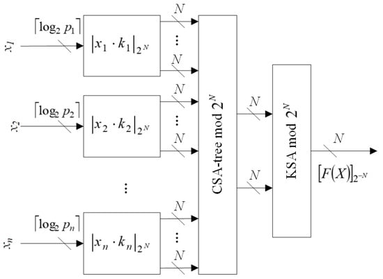
Figure 3.
The scheme of positional characteristics calculation based on CRTf.
3. Simulation of the Proposed Algorithm
It follows from the analysis of the modular division scheme that the comparison and sign detection unit is the main component determining its computational complexity. This unit can be implemented based on the CRT, MRNS, or CRT with fractions. We have considered the models of all three types.
The experimental simulation has been performed using ISE Design Suite 14.7. Kintex-7 KC705 XC7K70T-2FBG676 without DSP48E1B blocks has been chosen as the goal of compilation. This FPGA contains 10,250 slices and 300 input–output blocks. During the simulation, we varied the digit capacity of the moduli under a fixed number of bases. For each type of the model, same prime bases of a given capacity have been selected; in particular, four bases with module bits 5, 9, 13, 17, 21, and 25. The dynamic range of the system is approximately the product of the number of bases and their digit capacities. Only the bottleneck of the RNS division algorithm was implemented in hardware. The remaining parts of the division algorithm are very similar to the division operation in the standard IEEE library “ieee.numeric_std.all” and require approximately the same amount of resources in hardware implementation. Figure 4 shows the resource usage graph of this FPGA with different capacity moduli for each type of the model. Table 1 shows detailed resource utilization for all approaches considered.
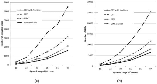
Figure 4.
FPGA Kintex-7 KC705 XC7K70T-2FBG676 resource usage by selected calculation basis: (a) number of occupied Slices, (b) number of LUTs.

Table 1.
Resources utilization and total delay.
All the considered algorithms were implemented on the corresponding FPGA. The architectures for CRT and MRC from [4] were simulated for comparison. In addition, the results for the division algorithm in the weighted numeric system (WNS) are also presented. For division in the WNS, an algorithm from standard IEEE library “ieee.numeric_std.all” was implemented. The pipeline in the binary division is implemented like in [26]. These results clearly show the fact that the additional circuit logic for the proposed method using CRT with fractions does not exceed 25% of the WNS division algorithm costs.
We will comprehend the scheme latency as the maximum time spent by an arbitrary signal to run over the whole scheme from a certain input to a certain output. Latency estimation allows describing the performance of the suggested algorithm, including the working frequency of the scheme. For each type of model, Figure 5 presents the working frequency of the scheme for the base systems with different digit capacities of the moduli.
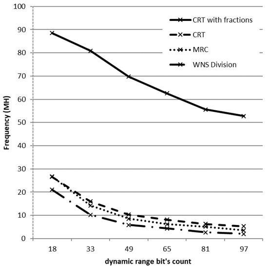
Figure 5.
Frequency as a function of dynamic range bit count.
As an example, consider a 64-bit capacity as the most widespread in modern computer systems. To write numbers in this system, it suffices to represent each of the four moduli as a 16- or 17-bit number. Let the set of moduli be {65537, 65539, 65543, 65551}. The range of this set forms a 65-bit number, which covers 64-bit capacity. Here, the approximate method requires only 689 slices, whereas the orthogonal basis method and the improved MRNS scheme require 1457 and 865 slices, respectively. On the other hand, the working frequency of the approximate method reaches 62.5 MHz, which is 7.6 times faster than the CRT-based restoration and 10.1 times faster than the improved MRNS method. Note that the advantages of the approximate method over these approaches remain in force for higher digit capacities, too.
4. Conclusions
The new algorithm described in this paper speeds up the modular division procedure in the RNS representation in comparison with the well-known analogs. This fact can be explained by the rather simple structure of the algorithm containing uncomplicated operations, namely, addition and shift (for quotient approximation), as well as shift and subtraction (for quotient refinement). Owing to CRT usage with fractions, the new algorithm does not include such operations as modular remainder calculation and number conversion into the mixed radix number system (MRNS) representation. The simulation of the algorithm on FPGA Kintex-7 has demonstrated a considerable reduction in hardware costs and an appreciable gain in speed as against the algorithms based on the CRT and MRNS representations.
Currently, this is the best hardware implementation of the general modular division. In comparison with the well-known algorithms, the suggested algorithm guarantees smaller hardware and time costs by a close connection between architectural calculations and hardware implementation. As a result, the computational complexity of modular division has been essentially decreased. The new algorithm is remarkable for easy implementation, thereby requiring fewer calculations than its well-known analogs.
A promising direction of further research is to find fast algorithms for several problem-causing operations in the RNS, namely, RNS-MRNS conversion and the optimal choice of RNS moduli within different ranges for specific applications. Each of the directions would promote the development of this field of computational mathematics owing to new RNS applications.
Author Contributions
Conceptualization, D.K., P.L., and N.C.; data curation, M.B. and I.L.; formal analysis, M.D.; funding acquisition, D.K.; investigation, A.L., A.N., M.V., and A.V.; methodology, P.L.; project administration, N.C.; resources, M.B. and I.L.; software, A.N., M.V., and A.V.; supervision, D.K. and P.L.; validation, M.D. and A.L.; visualization, A.V., M.V., and A.N.; writing—original draft preparation, N.C., P.L., and M.B.; writing—review and editing, D.K. and P.L. All authors have read and agreed to the published version of the manuscript.
Funding
This research was funded by the grant of the Russian Science Foundation (Project №19-19-00566).
Conflicts of Interest
The authors declare no conflicts of interest.
References
- Omondi, A.; Premkumar, B. Residue Number Systems: Theory and Implementation; Imperial College Press: London, UK, 2007. [Google Scholar]
- Szabo, N.S.; Tanaka, R.I. Residue Arithmetic and Its Applications to Computer Technology; McGraw-Hill: New York, NY, USA, 1967. [Google Scholar]
- Molahosseini, A.S.; Sorouri, S.; Zarandi, A.A.E. Research challenges in next-generation residue number system architectures. In Proceedings of the 7th International Conference on Computer Science & Education (ICCSE), Melbourne, Australia, 14–17 July 2012; pp. 1658–1661. [Google Scholar] [CrossRef]
- Mohan, P.V.A. Residue Number Systems: Theory and Applications; Birkhäuser: Basel, Switzerland, 2016. [Google Scholar]
- Chervyakov, N.I.; Lyakhov, P.A.; Nagornov, N.N.; Kaplun, D.I.; Voznesenskiy, A.S.; Bogayevskiy, D.V. Implementation of Smoothing Image Filtering in the Residue Number System. In Proceedings of the 2019 8th Mediterranean Conference on Embedded Computing (MECO), Budva, Montenegro, 10–14 June 2019; pp. 1–4. [Google Scholar]
- Younes, D.; Steffan, P. A comparative study on different moduli sets in residue number system. In Proceedings of the International Conference on Computer Systems and Industrial Informatics (ICCSII), Sharjah, UAE, 18–20 December 2012; pp. 1–6. [Google Scholar] [CrossRef]
- Nakahara, H.; Nakanishi, H.; Iwai, K.; Sasao, T. An FFT circuit for a spectrometer of a radio telescope using the nested RNS including the constant division. ACM SIGARCH Comput. Archit. News 2017, 4, 44–49. [Google Scholar] [CrossRef]
- Chren, W.A., Jr. A new residue number division algorithm. Comput. Math. Appl. 1990, 19, 13–29. [Google Scholar] [CrossRef]
- Chiang, J.-S.; Lu, M. A general Division Algorithm for Residue Number Systems. In Proceedings of the 10th IEEE Symposium on Computer Arithmetic, Grenoble, France, 26–28 June 1991. [Google Scholar] [CrossRef]
- Bigou, K.; Tisserand, A. Binary-ternary plus-minus modular inversion in rns. IEEE Trans. Comput. 2016, 65, 3495–3501. [Google Scholar] [CrossRef]
- Lu, M.; Chiang, J.-S. A novel division algorithm for Residue Number Systems. IEEE Trans. Comput. 1992, 41, 1026–1032. [Google Scholar] [CrossRef]
- Hung, C.Y.; Parhami, B. Fast RNS division algorithms for fixed divisors with application to RSA encryption. Inf. Process. Lett. 1994, 51, 163–169. [Google Scholar] [CrossRef]
- Hung, C.Y.; Parhami, B. An Approximate Sign Detection Method for Residue Numbers and its Application to RNS Division. Comput. Math. Appl. 1994, 27, 23–35. [Google Scholar] [CrossRef]
- Hiasat, A.A.; Abdel-Aty-Zohdy, H.S. Design and implementation of an RNS division algorithm. In Proceedings of the 13th IEEE Symposium on Computer Arithmetic, Asilomar, CA, USA, 6–9 July 1997; pp. 240–249. [Google Scholar] [CrossRef]
- Bajard, J.-C.; Didier, L.-S.; Muller, J.-M. A new Euclidean division algorithm for residue number systems. J. VLSI Signal Process. Syst. Signal Image Video Technol. 1998, 19, 167–178. [Google Scholar] [CrossRef]
- Hiasat, A.A.; Abdel-Aty-Zohdy, H.S. Semi-Custom VLSI Design and Implementation of a New Efficient RNS Division Algorithm. Comput. J. 1999, 42, 232–240. [Google Scholar] [CrossRef]
- Gorodecky, D.; Villa, T. Efficient Implementation of Modular Division by Input Bit Splitting. In Proceedings of the 2019 IEEE 26th Symposium on Computer Arithmetic (ARITH), Kyoto, Japan, 10–12 June 2019; IEEE: Piscataway, NJ, USA, 2019; pp. 54–60. [Google Scholar]
- Talahmeh, S.; Siy, P. Arithmetic division in RNS using Galois Field GF (p). Comput. Math. Appl. 2000, 39, 227–238. [Google Scholar] [CrossRef]
- Yang, Y.H.; Chang, C.C.; Chen, C.Y. A high-speed division algorithm in residue number system using parity-checking technique. Int. J. Comput. Math. 2004, 81, 775–780. [Google Scholar] [CrossRef]
- Chang, C.-C.; Lai, Y.-P. A division algorithm for residue numbers. Appl. Math. Comput. 2006, 172, 368–378. [Google Scholar] [CrossRef]
- Chang, C.-C.; Yang, J.-H. A division algorithm using bisection method in residue number system. Int. J. Comput. Consum. Control (IJ3C) 2013, 2, 59–66. [Google Scholar]
- Chervyakov, N.; Lyakhov, P.; Babenko, M.; Nazarov, A.; Deryabin, M.; Lavrinenko, I.; Lavrinenko, A. A High-Speed Division Algorithm for Modular Numbers Based on the Chinese Remainder Theorem with Fractions and Its Hardware Implementation. Electronics 2019, 8, 261. [Google Scholar] [CrossRef]
- Hitz, M.A.; Kaltofen, E. Integer division in residue number systems. IEEE Trans. Comput. 1995, 44, 983–989. [Google Scholar] [CrossRef]
- Knuth, D. The Art of Computer Programming, Volume 1: Fundamental Algorithms, 3rd ed.; Addison-Wesley Professional: Boston, MA, USA, 1997. [Google Scholar]
- Kogge, P.M.; Stone, H.S. A Parallel Algorithm for the Efficient Solution of a General Class of Recurrence Equations. IEEE Trans. Comput. 1973, 786–793. [Google Scholar] [CrossRef]
- Parhami, B. Computer Arithmetic: Algorithms and Hardware Designs; Oxford University Press: Oxford, UK, 2010; ISBN 9780195328486. [Google Scholar]
© 2020 by the authors. Licensee MDPI, Basel, Switzerland. This article is an open access article distributed under the terms and conditions of the Creative Commons Attribution (CC BY) license (http://creativecommons.org/licenses/by/4.0/).