Maximum Correntropy Criterion Based l₁-Iterative Wiener Filter for Sparse Channel Estimation Robust to Impulsive Noise

Abstract

In this paper, we propose a new sparse channel estimator robust to impulsive noise environments. For this kind of estimator, the convex regularized recursive maximum correntropy (CR-RMC) algorithm has been proposed. However, this method requires information about the true sparse channel to find the regularization coefficient for the convex regularization penalty term. In addition, the CR-RMC has a numerical instability in the finite-precision cases that is linked to the inversion of the auto-covariance matrix. We propose a new method for sparse channel estimation robust to impulsive noise environments using an iterative Wiener filter. The proposed algorithm does not need information about the true sparse channel to obtain the regularization coefficient for the convex regularization penalty term. It is also numerically more robust, because it does not require the inverse of the auto-covariance matrix.

1. Introduction

In many signal processing applications [1,2,3,4], we find various sparse channels in which most of the impulse responses are close to zero and only some of them are large. In recent years, many kinds of sparse adaptive filtering algorithms have been proposed for sparse system estimation, including recursive least squares (RLS)-based [5,6,7,8,9] and least mean square (LMS)-based algorithms [10,11,12,13,14]. It is generally known that RLS-based algorithms have faster convergence and less error after convergence than LMS-based algorithms [15]. However, there are fewer RLS-based than LMS-based algorithms. Among these, the convex regularized recursive least squares (CR-RLS) proposed by Eksioglu [6] is a full recursive convex regularized RLS like a typical RLS.

While the aforementioned algorithms typically show good performance in a Gaussian noise environment, their performance deteriorates in a nonGaussian noise environment such as an impulsive noise environment. Recently, the maximum correntropy criterion (MCC) [16,17,18,19] has been successfully applied to various adaptive algorithms robust to impulsive noise. Current studies in robust sparse adaptive methods have resulted in the development of CR-RLS-based algorithms with MCC [20,21], and showed strong robustness under impulsive noise. However, CR-RLS used in [20,21] is not practical when determining the regularization coefficient for the sparse regularization term because CR-RLS [6] needs information about the true channel when calculating the regularization coefficients. In addition, MCC CR-RLS algorithms (so called convex regularized recursive maximum correntropy (CR-RMC)) [20,21] include the inversion of the auto-covariance matrix, which is linked to the numerical instability in finite-precision environments [15].

The recursive inverse (RI) algorithm [22,23] and the iterative Wiener filter (IWF) algorithm [24] have recently been proposed. RI and IWF have the same structure besides a step size calculation. They perform similarly to the conventional RLS algorithm in terms of convergence and mean squared error, without using the inverse of the auto-covariance matrix. Therefore, RI [22,23] and IWF [24] can be considered algorithms without the numerical instability of RLS.

This paper proposes a sparse channel estimation algorithm robust to impulse noise using IWF and maximum correntropy criterion with l₁-norm regularization. The proposed algorithm includes a new regularization coefficient calculation method for l₁-norm regularization that does not require information about true channels. In addition, the proposed algorithm has numerical stability because it does not include inverse matrix calculation.

In Section 2 of this paper, we derive the new algorithm using IWF. In Section 3, we provide simulation results that show the performance of the proposed algorithm. In Section 4, we note our conclusions.

2. MCC l₁-IWF Formulation

In the channel estimation problem, we assume that at time instant n the observed signal $y(n)$ is the result of the input signal $x(k)$ sequence passing through the system $w_o={[w_0,\cdots ,w_{M-1}]}^T$ in the M-dimensional finite impulse response (FIR) format. Especially, in the sparse channel estimation problem, we assume that the system response w is sparse.

In the adaptive channel estimation, we apply an M dimensional channel $w(k)$ to the same dimensional signal vector $x(k)$, estimate an output $\widehat{y}(k)=x^T(k)w(k)$, and calculate the error signal $e(k)=y(k)+n(k)-\widehat{y}(k)=\tilde{y}(k)-\widehat{y}(k)$, where $y(k)$ is the output of the actual system, $\widehat{y}(k)$ is the estimated output, and $n(k)$ is the measurement noise. Especially, the measurement noise is nonGaussian.

To estimate the channel in nonGaussian noise, we define an MCC cost function with exponential forgetting factor λ shown in (1) [20,21] and minimize it adaptively.

$$\underset{\widehat{w}(n)}{\mathrm{minimize}}\left\{{\displaystyle \sum _{m=0}^n{\lambda }^{n-m}\exp \left(-\frac{{\left(y(m)-\widehat{w}{(n)}^{T}x(m)\right)}^2}{2{\sigma }^2}\hspace{0.33em}\right),}\hspace{0.33em}\mathrm{s}.\mathrm{t}.\hspace{0.33em}{‖\widehat{w}(n)‖}_1\le c\right\}\hspace{0.33em},$$

(1)

where $\widehat{w}(n)={\left[{\widehat{w}}_0(n),\cdots ,{\widehat{w}}_{M-1}(n)\right]}^T$, $x(m)={\left[x(m),x(m-1),\cdots ,x(m-M+1)\right]}^T$, $\lambda$ is a forgetting factor, and ${‖\widehat{w}(n)‖}_1\triangleq {\displaystyle {\sum }_{k=0}^{M-1}\left|{\widehat{w}}_k(n)\right|}$. The Lagrangian for (1) becomes

$$J\left(\widehat{w}(n),\gamma (n)\right)=\zeta \left(\widehat{w}(n)\right)+\gamma (n)\left({‖\widehat{w}(n)‖}_1-c\right),$$

(2)

where $\zeta \left(\widehat{w}(n)\right)={\displaystyle \sum _{m=0}^n{\lambda }^{n-m}\exp \left(-\frac{{\left(y(m)-\widehat{w}{(n)}^{T}x(m)\right)}^2}{2{\sigma }^2}\hspace{0.33em}\right),}$ and $\gamma (n)$ is a real-valued Lagrangian multiplier. We minimize the regularized cost function to find the optimal vector in the same way that IWF was derived [24].

The regularized cost function is convex and nondifferentiable; therefore, subgradient analysis replaces the gradient. When denoting a subgradient vector of $f$ at $\widehat{w}$ with ${\nabla }^{s}f(\widehat{w})$, the subgradient vector of $J(\widehat{w}(n),\gamma (n))$ with respect to $\widehat{w}(n)$ can be written as follows:

$${\nabla }^{s}J\left(\widehat{w}(n),\gamma (n)\right)=\nabla \zeta \left(\widehat{w}(n)\right)+\gamma (n){\nabla }^s\left({‖\widehat{w}(n)‖}_1\right).$$

(3)

Hence, for the optimal $\widehat{w}(n)$ minimizing $J(\widehat{w}(n),\gamma (n))$, we set the subgradient of $J(\widehat{w}(n),\gamma (n))$ to 0 at the optimal point. When evaluating the gradient $\nabla \zeta (\widehat{w}(n))$, we can derive a gradient vector as (4).

$${\nabla }^{s}J\left(\widehat{w}(n),\gamma (n)\right)=\frac{1}{{\sigma }^2}\left(\Phi (n)\widehat{w}(n)-r(n)\right)+\gamma (n)\mathrm{sgn}\left(\widehat{w}(n)\right)=g_n,$$

(4)

where $e(n)=y(n)-\widehat{w}{(n)}^{T}x(n)$, $\Phi (n)={\displaystyle \sum _{m=0}^n{\lambda }^{n-m}x(m)x{(m)}^T}=\lambda \Phi (n-1)+\exp \left(-\frac{e{(n)}^2}{2{\sigma }^2}\right)x(n)x{(n)}^T$, $r(n)={\displaystyle \sum _{m=0}^n{\lambda }^{n-m}y(m)x(m)}=\lambda r(n-1)+\exp \left(-\frac{e{(n)}^2}{2{\sigma }^2}\right)y(n)x(n)$, and ${\nabla }^s\left({{\displaystyle ‖\widehat{w}(n)‖}}_1\right)=\mathrm{sgn}\left(\widehat{w}(n)\right)$ [6]. Using Equation (4), we can obtain the update expression for $\widehat{w}(n)$ as (5).

$$\widehat{w}(n+1)=\widehat{w}(n)-{\mu }_n{\nabla }^{s}J\left(\widehat{w}(n),\gamma (n)\right)=\widehat{w}(n)-{\mu }_n{g}_n$$

(5)

To get the step size ${\mu }_n$, we find the ${\mu }_n$ that minimizes exponentially averaged a posteriori error energy, $J\left(\widehat{w}(n+1),\gamma (n)\right)$, where a posteriori error is $e(n)=y(n)-\widehat{w}{(n+1)}^{T}x(n)\hspace{0.33em}$.

$$\begin{array}{ll}{\nabla }_{\mu }J\left(\widehat{w}(n+1),\gamma (n)\right)& =-\frac{1}{{\sigma }^2}\widehat{w}{(n+1)}^T\Phi (n)g_n+\frac{1}{{\sigma }^2}r{(n)}^T{g}_n-\gamma (n){\nabla }^s{\left({‖\widehat{w}(n+1)‖}_1\right)}^T{g}_n\\ & \cong -\frac{1}{{\sigma }^2}\widehat{w}{(n+1)}^T\Phi (n)g_n+\frac{1}{{\sigma }^2}r{(n)}^T{g}_n-\gamma (n){\nabla }^s{\left({‖\widehat{w}(n)‖}_1\right)}^T{g}_n\\ & =-\frac{1}{{\sigma }^2}\widehat{w}{(n+1)}^T\Phi (n)g_n+\frac{1}{{\sigma }^2}r{(n)}^T{g}_n-\gamma (n)\mathrm{sgn}{(\widehat{\mathbf{w}}(n))}^T{g}_n.\end{array}$$

(6)

Substituting Equation (5) into Equation (6), we get

$${\nabla }_{\mu }J\left(\widehat{w}(n+1),\gamma (n)\right)=-\frac{1}{{\sigma }^2}\widehat{w}{(n)}^T\Phi (n)g_n+\frac{1}{{\sigma }^2}{\mu }_n{g}_n^T\Phi (n)g_n+\frac{1}{{\sigma }^2}r{(n)}^T{g}_n-\gamma (n)\mathrm{sgn}{\left(\widehat{w}(n)\right)}^T{g}_n.$$

(7)

To find ${\mu }_n$, we set ${\nabla }_{\mu }J\left(\widehat{w}(n),\gamma (n)\right)=0$, and

$${\mu }_n=\frac{\frac{1}{{\sigma }^2}\left(\widehat{w}{(n)}^T\Phi (n)-r{(n)}^T\right)g_n+\gamma (n)\mathrm{sgn}{\left(\widehat{w}(n)\right)}^T{g}_n}{\frac{1}{{\sigma }^2}{g}_n^T\Phi (n)g_n}={\sigma }^2\frac{g_n^T{g}_n}{g_n^T\Phi (n)g_n}$$

(8)

We have to derive regularization coefficient $\widehat{\gamma }(n)$ such that ${‖\widehat{w}(n+1)‖}_1=c$, i.e., the l₁-norm of vector $\widehat{w}(n+1)$ is preserved at all time steps of n. This can be represented by a flow equation in continuous time-domain in [25].

$$\frac{\partial {‖\widehat{w}(t)‖}_1}{\partial t}={\left(\frac{\partial {‖\widehat{w}(t)‖}_1}{\partial \widehat{w}}\right)}^T\frac{\partial \widehat{w}}{\partial t}={\left({\nabla }^s{‖\widehat{w}(t)‖}_1\right)}^T\frac{\partial \widehat{w}}{\partial t}=0\hspace{0.33em}.$$

(9)

Using a sufficiently small interval δ, the time derivative in (9) can be approximated as

$${\left({\nabla }^s{‖\widehat{w}(t)‖}_1\right)}^T\frac{\partial \widehat{w}}{\partial t}\cong {\left({\nabla }^s{‖\widehat{w}(n)‖}_1\right)}^T\frac{\left(\widehat{w}(n+1)-\widehat{w}(n)\right)}{\delta }=0\hspace{0.33em}.$$

(10)

Using (5) and (6), (10) becomes

$$\mathrm{sgn}{\left(\widehat{w}(n)\right)}^T\left(\widehat{w}(n+1)-\widehat{w}(n)\right)=\mathrm{sgn}{\left(\widehat{w}(n)\right)}^T(-{\mu }_n{g}_n)=0\hspace{0.33em}.$$

(11)

and

$$\mathrm{sgn}{\left(\widehat{w}(n)\right)}^T\left(\frac{1}{{\sigma }^2}\Phi (n)w(n)-\frac{1}{{\sigma }^2}r(n)+\gamma (n)\mathrm{sgn}\left(\widehat{w}(n)\right)\right)=0\hspace{0.33em}.$$

(12)

The regularization coefficient $\widehat{\gamma }(n)$ obtained from Equation (12) is as follows.

$$\gamma (n)=-\frac{\mathrm{sgn}{\left(\widehat{w}(n)\right)}^T\left(\Phi (n)w(n)-r(n)\right)}{{\sigma }^2\mathrm{sgn}{\left(\widehat{w}(n)\right)}^T\mathrm{sgn}\left(\widehat{w}(n)\right)}.$$

(13)

On the contrary, CR-RMC algorithm in [20] uses the same regularization coefficient as that in [6]. The regularization coefficient is shown in (14)

$$\widehat{\gamma }(n)=2\frac{\frac{tr\left({\Phi }^{-1}(n)\right)}{M}\left({{\displaystyle ‖\widehat{w}(n)‖}}_1-\rho \right)++\mathrm{sgn}{(\widehat{w}(n))}^T{\Phi }^{-1}(n)\epsilon (n)}{{{\displaystyle {\sigma }^2‖{\Phi }^{-1}(n)\mathrm{sgn}(\widehat{w}(n))‖}}_2^2},$$

(14)

where $\epsilon (n)=\tilde{w}(n)-\widehat{w}(n)$ and $\tilde{w}(n)$ is the solution to the normal equation, $\Phi (n)\tilde{w}(n)=r(n)$. In (14), the regularization coefficient has the parameter, $\rho$. In [6] and [20], the parameter was set as $\rho =f(w_{true})={{\displaystyle ‖w_{true}‖}}_1$, with $w_{true}$ indicating the impulse response of the true channel. There was no further discussion about how to set $\rho$. We summarize the algorithm in

Table 1. Summary of the l₁- iterative Wiener filter (IWF).

Initialization: $\Phi (0)$,$r(0)$,$\widehat{w}(0)$, ${\sigma }^2$.

For n = 1 …

$\Phi (n)=\lambda \Phi (n-1)+\exp \left(-\frac{e{(n)}^2}{2{\sigma }^2}\right)x(n)x{(n)}^T$

$r(n)=\lambda r(n-1)+\exp \left(-\frac{e{(n)}^2}{2{\sigma }^2}\right)y(n)x(n)$

$\gamma (n)=-\frac{\mathrm{sgn}{\left(\widehat{w}(n)\right)}^T\left(\Phi (n)w(n)-r(n)\right)}{{\sigma }^2\mathrm{sgn}{\left(\widehat{w}(n)\right)}^T\mathrm{sgn}\left(\widehat{w}(n)\right)}$

$g_n=\Phi (n)\widehat{w}(n)-r(n)+\gamma (n)\mathrm{sgn}\left(\widehat{w}(n)\right)$

${\mu }_n=\frac{g_{n-1}^T{g}_{n-1}}{g_{n-1}^T\Phi (n)g_{n-1}}$

$\widehat{w}(n+1)=\widehat{w}(n)-{\mu }_n{g}_n$

end

.

3. Simulation Results

In this section, we compare the sparse channel estimation performance between the proposed algorithm and the convex regularized recursive maximum correntropy (CR-RMC) [20]. In addition, the numerical robustness of the proposed algorithm is compared with that of CR-RMC in the finite-precision environments.

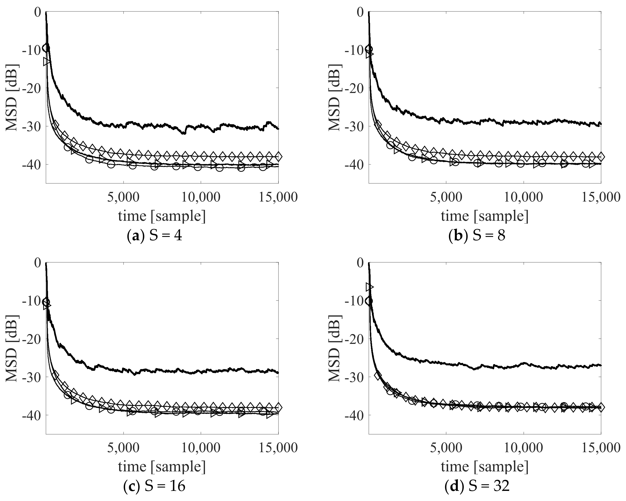
3.1. Estimation of Sparse Channels

In this experiment, we showed the sparse system estimation results. The simulation was performed under the same experimental conditions in [6]. The true system parameter $w_o$ had an order of M = 64. Out of the 64 coefficients, there were S nonzero coefficients. The nonzero coefficients were placed randomly, and the values of the coefficients were drawn from a $N\left(0,1/\mathrm{S}\right)\hspace{0.17em}$ distribution. The impulsive noise is generated according to the Gaussian mixture model [26]

$$p_v=\left(1-p_r\right)N\left(0,{\sigma }_1^2\right)+p_{r}N\left(0,{\sigma }_2^2\right)$$

(15)

where $N\left(0,{\sigma }_i^2\right)\hspace{0.17em}\left(i=1,\hspace{0.33em}2\right)$ denote the Gaussian distribution with zero-mean and variance ${\sigma }_i^2$. The $p_r$ denotes the occurrence probability of the Gaussian distribution with variance ${\sigma }_2^2$, which usually is much larger than ${\sigma }_1^2$ so as to generate the impulsive noises. The zero-mean Gaussian distribution with variance ${\sigma }_1^2$ generated the background noise, and the zero-mean Gaussian distribution with variance ${\sigma }_2^2$ (usually ${\sigma }_2^2\gg {\sigma }_1^2$) generated the impulsive noise with the probability $p_r$. In this experiment, we set the variance of ${\sigma }_1^2$ to 0.01 and generate the input signal so that SNR keeps 20dB. The other parameters were set as ${\sigma }_2^2=500$ and $p_r=0.01$.

We compare CR-RMC [20] using the true system response information and the proposed algorithm using a regularization factor that did not use the true system response. It also included the results of the MCC-RLS [27] and the conventional RLS without considering impulsive noise and sparsity. For the performance evaluation, we simulated the algorithms in the sparse impulse response for S = 4, 8, 16, 32.

Figure 1 illustrates the mean standard deviation (MSD) curves. The results show that the estimation performance of the proposed algorithm is similar to that of CR-RMC using the regularization factor referring to the true system impulse response. As expected, the conventional RLS produced the worst MSD in all cases.

Figure 1 confirms that, without a priori information about the true system impulse response, the proposed regularization factor works similarly to that of the regularization factor in CR-RMC using the true system impulse response information.

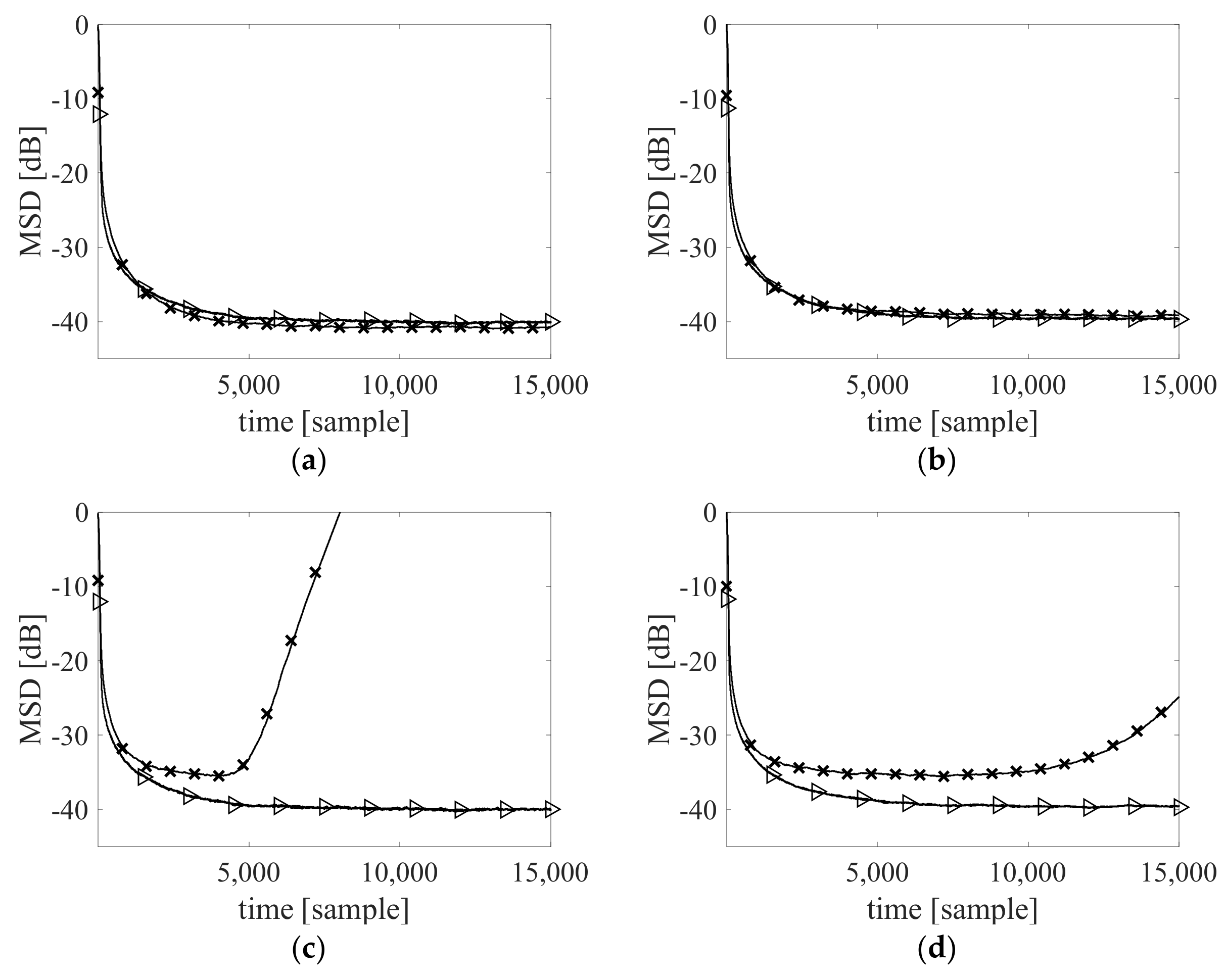
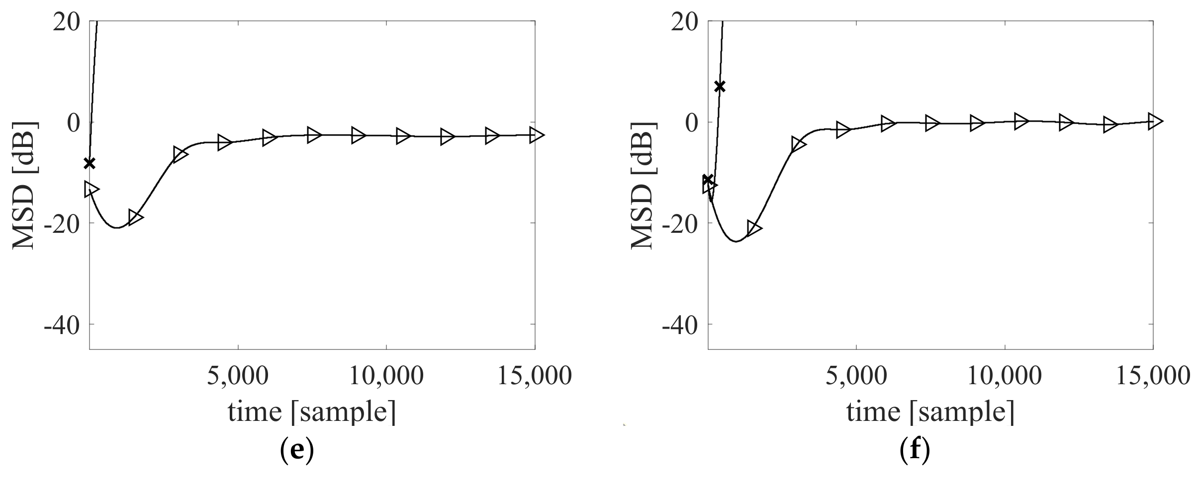
3.2. Numerical Robustness Experiment

In this experiment, we showed the proposed algorithm to be numerically more robust than CR-RMC in the finite-precision environments. We performed channel estimation with finite precision by quantization to show the numerical robustness [28]. The round-off error from the quantization with finite bits was accumulated and propagated through the inverse matrix operation of $\Phi (n)$, and, finally, explosive divergence occurred [15,28]. To illustrate this, we repeated numerical stability experiments, decreasing the quantization bit from 32 bits by 1 bit to find the quantization bits that started numerical instability in each algorithm while comparing and verifying the performance for the case of S = 4 and S = 16. In addition, the rest of the setup for the experiment was the same as Experiment 3.1.

Figure 2 shows the results of comparing the performance of the proposed algorithm and CR-RMC in terms of MSD with different numbers of quantization bits. Figure 2a,b shows the results when quantized to 32 bits. In this case, we can observe that the proposed algorithm as well as CR-RMC converges normally as Figure 1a,b. Figure 2 shows the results of comparing the performance of the proposed algorithm and CR-RMC in terms of MSD with different numbers of quantization bits. Figure 2a,b shows the results when quantized to 32 bits. In this case, we can observe that the proposed algorithm as well as CR-RMC converges normally as Figure 1a,b. Figure 2c,d shows the quantization results for 16 bits. In 16 bits, CR-RMC started numerical instability. Compared with the results of Figure 2a,b, it can be observed that quantized CR-RMC diverges due to the cumulative effect of the error of quantization noise. Figure 2e,f shows the quantization results for 11 bits. In 11 bits, the proposed algorithm also started numerical instability. If we consider the level of quantization error with signal to quantization noise ratio (SQNR), SQNR (dB) = 1.76 + 6.02 × bits [29], CR-RMC is stable at above 98.08 dB in SQNR. The proposed algorithm is stable at above 67.98 dB in SQNR. In other word, the proposed algorithm has 30.1 dB gain in numerical stability compared to CR-RMC.

The experimental results confirm that the proposed algorithm is numerically more robust than CR-RMC.

4. Conclusions

In this paper, this paper have proposed a sparse channel estimation algorithm robust to impulse noise using IWF and MCC with l₁-norm regularization. The proposed algorithm includes a regularization factor calculation algorithm without any requirement for a priori knowledge about the true system response. The simulation results show that the proposed algorithm works similarly to the CR-RMC algorithm with a regularization factor referring to the true system response information. In addition, simulation results show that the proposed algorithm is more robust against numerical error than the CR-RMC algorithm.

References

1. Loganathan, P.; Khong, A.W.; Naylor, P.A. A class of sparseness-controlled algorithms for echo cancellation. IEEE Trans. Audio Speech Lang. Process. 2003, 17, 1591–1601. [Google Scholar] [CrossRef]
2. Carbonelli, C.; Vedantam, S.; Mitra, U. Sparse channel estimation with zero tap detection. IEEE Trans. Wirel. Commun. 2007, 6, 1743–1763. [Google Scholar] [CrossRef] [Green Version]
3. Yousef, N.R.; Sayed, A.H.; Khajehnouri, N. Detection of fading overlapping multipath components. Signal Process. 2006, 86, 2407–2425. [Google Scholar] [CrossRef]
4. Singer, A.C.; Nelson, J.K.; Kozat, S.S. Signal processing for underwater acoustic communications. IEEE Commun. Mag. 2009, 47, 90–96. [Google Scholar] [CrossRef]
5. Babadi, B.; Kalouptsidis, N.; Tarokh, V. SPARLS: The sparse RLS algorithm. IEEE Trans. Signal Process. 2010, 58, 4013–4025. [Google Scholar] [CrossRef] [Green Version]
6. Eksioglu, E.M. RLS algorithm with convex regularization. IEEE Signal Process. Lett. 2011, 18, 470–473. [Google Scholar] [CrossRef]
7. Eksioglu, E.M. Sparsity regularised recursive least squares adaptive filtering. IET Signal Process. 2011, 5, 480–487. [Google Scholar] [CrossRef]
8. Das, B.; Chakraborty, M. Improved l0-RLS adaptive filter algorithms. Electron. Lett. 2017, 53, 1650–1651. [Google Scholar] [CrossRef]
9. Liu, L.; Zhang, Y.; Sun, D. VFF l1-norm penalised WL-RLS algorithm using DCD iterations for underwater acoustic communication. IET Commun. 2017, 11, 615–621. [Google Scholar] [CrossRef]
10. Li, Y.; Wang, Y.; Jiang, T. Norm-adaption penalized least mean square/fourth algorithm for sparse channel estimation. Signal Process. 2016, 128, 243–251. [Google Scholar] [CrossRef]
11. Jahromi, M.N.S.; Salman, M.S.; Hocanin, A. Convergence analysis of the zero-attracting variable step-size LMS algorithm for sparse system identification. Signal Image Video Process. 2013, 9, 1353–1356. [Google Scholar] [CrossRef]
12. Li, Y.; Wang, Y.; Jiang, T. Sparse-aware setmembership NLMS algorithms and their application for sparse channel estimation and echo cancelation. AEU-Int. J. Electron. Commun. 2016, 70, 895–902. [Google Scholar] [CrossRef]
13. Gu, Y.; Jin, J.; Mei, S. l0-norm constraint LMS algorithm for sparse system identification. IEEE Signal Process. Lett. 2009, 16, 774–777. [Google Scholar]
14. Chen, Y.; Gu, Y.; Hero, A.O. Sparse LMS for system identification. In Proceedings of the IEEE International Conference on Acoustics, Speech Signal Processing, Taipei, Taiwan, 19–24 April 2009; pp. 3125–3128. [Google Scholar]
15. Haykin, S. Adaptive Filter Theory, 5th ed.; Prentice Hall: Upper Saddle River, NJ, USA, 2014. [Google Scholar]
16. Liu, W.; Pokharel, P.P.; Principe, J.C. Correntropy: Properties and applications in non-Gaussian signal processing. IEEE Trans Signal Process. 2007, 55, 5286–5298. [Google Scholar]
17. Chen, B.; Xing, L.; Liang, J.; Zheng, N.; Principe, J.C. Steady-state mean-square error analysis for adaptive filtering under the maximum correntropy criterion. IEEE Signal Process. Lett. 2014, 21, 880–884. [Google Scholar]
18. Ma, W.; Qu, H.; Gui, G.; Xu, L.; Zhao, J.; Chen, B. Maximum correntropy criterion based sparse adaptive filtering algorithms for robust channel estimation under non-Gaussian environments. J. Frankl. Inst. 2015, 352, 2708–2727. [Google Scholar] [CrossRef] [Green Version]
19. Chen, B.; Xing, L.; Zhao, H.; Zheng, N.; Principe, J.C. Generalized correntropy for robust adaptive filtering. IEEE Trans. Signal Process. 2016, 64, 3376–3387. [Google Scholar] [CrossRef] [Green Version]
20. Zhang, X.; Li, K.; Wu, Z.; Fu, Y.; Zhao, H.; Chen, B. Convex regularized recursive maximum correntropy algorithm. Signal Process. 2016, 129, 12–16. [Google Scholar] [CrossRef]
21. Ma, W.; Duan, J.; Chen, B.; Gui, G.; Man, W. Recursive generalized maximum correntropy criterion algorithm with sparse penalty constraints for system identification. Asian J. Control 2017, 19, 1164–1172. [Google Scholar] [CrossRef]
22. Ahmad, M.S.; Kukrer, O.; Hocanin, A. Recursive inverse adaptive filtering algorithm. Digit. Signal Process. 2011, 21, 491–496. [Google Scholar] [CrossRef]
23. Salman, M.S.; Kukrer, O.; Hocanin, A. Recursive inverse algorithm: Mean-square-error analysis. Digit. Signal Process. 2017, 66, 10–17. [Google Scholar] [CrossRef]
24. Xi, B.; Liu, Y. Iterative Wiener Filter. Electron. Lett. 2013, 49, 343–344. [Google Scholar] [CrossRef]
25. Khalid, S.; Abrar, S. Blind adaptive algorithm for sparse channel equalization using projections onto lp-ball. Electron. Lett. 2015, 51, 1422–1424. [Google Scholar] [CrossRef]
26. Wang, W.; Zhao, J.; Qu, H.; Chen, B. A correntropy inspired variable step-size sign algorithm against impulsive noises. Signal Process. 2017, 141, 168–175. [Google Scholar] [CrossRef]
27. Ma, W.; Qu, H.; Zhao, J. Estimator with forgetting factor of correntropy and recursive algorithm for traffic network prediction. In Proceedings of the 2013 25th Chinese Control and Decision Conference (CCDC), Guiyang, China, 25–27 May 2013; pp. 490–494. [Google Scholar]
28. Sayed, A.H. Fundamentals of Adaptive Filtering; John Wiley & Sons, Inc.: Hoboken, NJ, USA, 2003; pp. 775–803. [Google Scholar]
29. Proakis, J.G.; Manolakis, D.K. Digital Signal Processing, 4th ed.; Pearson Education Limited: London, UK, 2014; p. 35. [Google Scholar]
Figure 1. Steady state MSD for S = 4, 8, 16, 32 (-⊳-: the proposed algorithm, -∘-: convex regularized recursive maximum correntropy (CR-RMC), -⋄-: maximum correntropy criterion (MCC)- recursive least squares (RLS), solid line: conventional RLS without considering impulsive noise and sparsity): (a) S = 4, (b) S = 8, (c) S = 16, (d) S = 32.
Applsci 10 00743 g001
Figure 2. Results of numerical robustness experiment (-⊳-: the proposed algorithm, -x-: CR-RMC): (a) S = 4 case quantized by 32 bits; (b) S = 16 case quantized by 32 bits; (c) S = 4 case quantized by 16 bits; (d) S = 16 case quantized by 16; (e) S = 4 case quantized by 11 bits; and (f) S = 16 case quantized by 11 bits.
Applsci 10 00743 g002aApplsci 10 00743 g002b