A Novel Spectral–Spatial Classification Method for Hyperspectral Image at Superpixel Level

Featured Application

The proposed methodology can be applied in the field of agricultural land use and land cover classification, precision agriculture, and environmental monitoring.

Abstract

Although superpixel segmentation provides a powerful tool for hyperspectral image (HSI) classification, it is still a challenging problem to classify an HSI at superpixel level because of the characteristics of adaptive size and shape of superpixels. Furthermore, these characteristics of superpixels along with the appearance of noisy pixels makes it difficult to appropriately measure the similarity between two superpixels. Under the assumption that pixels within a superpixel belong to the same class with a high probability, this paper proposes a novel spectral–spatial HSI classification method at superpixel level (SSC-SL). Firstly, a simple linear iterative clustering (SLIC) algorithm is improved by introducing a new similarity and a ranking technique. The improved SLIC, specifically designed for HSI, can straightly segment HSI with arbitrary dimensionality into superpixels, without consulting principal component analysis beforehand. In addition, a superpixel-to-superpixel similarity is newly introduced. The defined similarity is independent of the shape of superpixel, and the influence of noisy pixels on the similarity is weakened. Finally, the classification task is accomplished by labeling each unlabeled superpixel according to the nearest labeled superpixel. In the proposed superpixel-level classification scheme, each superpixel is regarded as a sample. This obviously greatly reduces the data volume to be classified. The experimental results on three real hyperspectral datasets demonstrate the superiority of the proposed spectral–spatial classification method over several comparative state-of-the-art classification approaches, in terms of classification accuracy.

1. Introduction

Hyperspectral image (HSI) classification is one of the most active and attractive topics in the field of remote sensing. Compared with multispectral sensors, hyperspectral sensors can capture more abundant information of land cover, such as agricultural crop types. This detailed spectral–spatial information will greatly increase the discriminative ability of HSI. In recent years, HSI classification has been successfully applied to precision agriculture [1,2], environment monitoring [3,4], ocean exploration [5], object detection [6,7], and so on. However, it continues to be a challenging problem to develop new effective spectral–spatial methods to classify HSI accurately, due to its high dimension, large data volume, massive noisy pixels, and few training samples.

HSI classification needs to assign a meaningful class label to each pixel within the image according to the spectral feature or spectral–spatial information. A large number of effective HSI classification techniques have been developed in the past decades. Early HSI classification methods mainly used the spectral features to classify hyperspectral data [8,9,10,11,12]. Although the classification results obtained by these methods may not be good enough, this is a successful attempt to apply the machine learning method to hyperspectral remote sensing. Lately, spatial structure information has been gradually taken into account in some pixel-based classification approaches [13,14,15,16,17,18,19,20], aiming at getting better classification results. Generally speaking, the purpose of introducing spatial information into the process of classification can be roughly understood as denoising HSI in preprocessing [21,22,23,24], defining the novel similarity between a pair of pixels [25,26], reducing dimensionality [27], improving the classification map in post-processing [28,29,30], or their combinations. From the point of view of classification accuracy, the existing literatures show that some spectral–spatial HSI classification methods do have good classification performance.

In recent times, more attention has been paid to spectral–spatial HSI classification approaches based on superpixel in remote sensing. Unlike the fixed-size window commonly used in the Markov random field technique [31,32], a superpixel is a homogeneous region with adaptive shape and size. Specifically, superpixel-based classification methods first segment HSI into superpixels, and then integrate various techniques and classifiers to process hyperspectral data [33,34,35,36]. For example, the SuperPCA method developed an intrinsic low dimensional feature of HSI by using principal component analysis (PCA) on each superpixel [35]. Zhang et al. presented an effective classification method by using the joint sparse representation on different superpixels [36]. On the basis of multiscale superpixels and guided filter, Dundar and Ince depicted a spectral–spatial HSI classification method [24]. In addition, the homogeneity of superpixels together with the majority voting strategy were also adopted to improve the classification map in some spectral–spatial HSI classification methods [37,38,39]. These superpixel-based HSI classification methods at pixel level utilize the spatial information of HSI detected by the superpixels to improve the performance of classification algorithms.

Very recently, under the assumption that pixels within a superpixel should share the same class label, two superpixel-level HSI classification methods have been proposed. Based on an affine hull model and set-to-set distance, Lu et al. developed a spectral–spatial HSI classification method at superpixel level [40]. Sellars et al. proposed a graph-based semi-supervised classification technique for HSI by defining the weight between two adjacent superpixels [41]. The classification at superpixel level is, to some degree, a reduction of pixels, which may greatly reduce the number of objects in the classification process. To our knowledge, most of the existing HSI classification methods based on superpixels are pixel level, and few of them are superpixel level. Therefore, it is significant to propose new powerful and effective spectral–spatial classification approaches at superpixel level in the field of remote sensing.

For the HSI classification method at superpixel level, two key problems need to be considered: (i) How to segment the HSI into the superpixels? (ii) How to properly measure the similarity between two superpixels? As for the first problem, two representative segmentation algorithms, simple linear iterative clustering algorithm (SLIC) [42] and the entropy rate superpixel (ERS) [43], are usually applied to divide the given HSI into multiple non-overlapping homogeneous regions. Although these two methods show good performance in the segmentation of HSI, the PCA method must be performed in advance, and the problem of selecting the optimal parameter in SLIC and ERS is also encountered. In addition, it is fundamentally important to properly measure the similarity between a pair of superpixels in the superpixel-level HSI classifier because it is closely related to the classification results. However, the appropriate definition of the similarity between two superpixels is non-trivial, due to the complexity of spectra and spatial structure of the pixels in the superpixel.

To address the problems mentioned above, this study chooses SLIC as an attempt first because it has the advantages of fast calculation, convenient use, and accurate matching with the contour of objects [42]. By taking into account the spectrum differences of two pixels and their correlation, we introduce a new distance metric to measure the similarity between two pixels. Based on a novel sorting strategy and the suggested measurement, SLIC has been improved so that it can be straightly used to partition HSI into superpixels, without consulting PCA and requiring parameters. Compared with our earlier improvement of SLIC [28], the improved SLIC here has good computability and understanding. Furthermore, motivated by the idea of local mean-based pseudo nearest neighbor (LMPNN) rule, we also define a new metric to measure the similarity between a pair of superpixels. Specifically, we first adopt the LMPNN rule to calculate the distance from a pixel to a superpixel. Then the superpixel-to-superpixel similarity is obtained by extending the LMPNN rule to the case of set-to-set. Under the assumption that pixels within a superpixel should be the same class label, the classification is carried out by marking each unlabeled superpixel as the same label as its closest labeled superpixel.

The main contributions of the proposal are concluded as following:

• The SLIC algorithm is improved so that it can be directly used to divide any dimensional HSI into superpixels without using PCA and parameters.
• The superpixel-to-superpixel similarity is defined properly, which is unrelated to the shape of superpixel.
• A novel spectral–spatial HSI classification method at superpixel level is proposed.

2. The Proposed HSI Classification Method at Superpixel Level

2.1. SLIC Algorithm and Its Improvement

Superpixel segmentation is a powerful and important technique in computer vision and image processing. Some typical segmentation algorithms are SLIC [42], ERS [43], watersheds [44], MeanShift [45], Turbopixels [46], and so on. Among them, SLIC, proposed by Achanta et al. in 2010 [42], is easy to use and understand, and; therefore, is one of the most popular segmentation algorithms. This algorithm adopts the strategy of local k-means clustering to generate the compact superpixels of color images.

For a given color image in the CIELAB color space, each pixel in this color image can be represented as $\left(l_i,a_i,b_i,p_i,q_i\right)$ (I = 1, 2, …, N), which is composed of color value $\left(l_i,a_i,b_i\right)$ and coordinate $\left(p_i,q_i\right)$. The image will be approximately segmented into N/s² regions with a roughly equal size by a predetermined segmentation scale $s$. To ensure the segmentation quality, the gradient descent technique was used to select the initial N/s² centers to avoid them on edges or noisy pixels. Aiming at improving the calculation speed, the k-means clustering was carried out locally in an area of $2\mathrm{s}\times 2\mathrm{s}$ centered on the tested pixel, rather than the whole image. The following metric was adopted to measure the similarity of a pair of pixels in SLIC algorithm [42],

$$d_{lab}=\sqrt{{\left(l_i-l_j\right)}^2+{\left(a_i-a_j\right)}^2+{\left(b_i-b_j\right)}^2},$$

(1)

$$d_{pq}=\sqrt{{\left(p_i-p_j\right)}^2+{\left(q_i-q_j\right)}^2},$$

(2)

$$d=\sqrt{d_{lab}^2+m^2{\left(\frac{d_{pq}}{s}\right)}^2},$$

(3)

where $d_{lab}$ and $d_{pq}$ denote the color difference and spatial distance of a pair of pixels, respectively; the balance parameter m in Equation (3) is to weigh the importance between $d_{lab}$ and $d_{pq}$.

It is clear that the classical SLIC algorithm cannot be applied directly to superpixel segmentation of HSI. This is because different magnitudes between bands risk to make the distance depending only on high magnitude wavelengths discarding the low magnitude ones. In addition, if the color distance $d_{lab}$ in Equation (1) is replaced directly by spectral distance, huge spectral difference among hundreds of bands will cause enormous difficulty to the balance of two terms in Equation (3). Experimental results show that this method cannot get a satisfactory segmentation result. Although we can use classic SLIC to split HSI into superpixels by pre-executing PCA, this means that the more knowledge and the optimal parameter values are required.

To address the aforementioned problem, in what follows, we will put forward an improved SLIC algorithm by introducing a novel technique and a new measurement. The improved SLIC, especially designed for segmenting HSI, can be straightforward used to superpixel segmentation of HSI with any dimensionality.

The improved SLIC algorithm is described as follows:

Let $\mathrm{HSI}=\left({\mathit{x}}_1, {\mathit{x}}_2,\cdots ,{\mathit{x}}_N\right)\subset R^{\mathrm{B}}$ be a hyperspectral dataset with N pixels; the spectral feature of pixel ${\mathit{x}}_i$ is represented by ${\mathit{x}}_i={\left(x_{i,1}, x_{i,2},\cdots ,x_{i,B}\right)}^T$; B is the number of bands. After carefully considering the spectral features of the pixels and the correlation between them, we would like to defined the spectral similarity of two pixels ${\mathit{x}}_i$ and ${\mathit{x}}_j$ as

$$S_{spec}\left(x_i,x_j\right)=\left(1-{\rho }_{i,j}\right){\left[{\sum }_{k=1}^B{\left(x_{i,k}-x_{j,k}\right)}^2\right]}^{\frac{1}{2}},$$

(4)

where ${\rho }_{i,j}$ is Pearson correlation coefficient calculated by

$${\rho }_{i,j}=\frac{\mathrm{B}{\sum }_{h=1}^{\mathrm{B}}{x}_{i,h}{x}_{j,h}-{\sum }_{h=1}^{\mathrm{B}}{x}_{i,h}{\sum }_{\mathrm{h}=1}^{\mathrm{B}}{x}_{j,h}}{\sqrt{\mathrm{B}{\sum }_{h=1}^{\mathrm{B}}{x}_{i,h}^2-{\left({\sum }_{h=1}^{\mathrm{B}}{x}_{i,h}\right)}^2}\sqrt{\mathrm{B}{\sum }_{h=1}^{\mathrm{B}}{x}_{j,h}^2-{\left({\sum }_{\mathrm{h}=1}^{\mathrm{B}}{x}_{j,h}\right)}^2}}.$$

(5)

The proposed spectral similarity $S_{spec}\left({\mathit{x}}_i,{\mathit{x}}_j\right)$ takes into account both spectral distance and correlation. In theory, the difference between two pixels can be measured better.

Suppose there are k centers around pixel ${\mathit{x}}_i$, ${\mathit{c}}_1,{\mathit{c}}_2,\cdots ,{\mathit{c}}_k$. Clustering in the improved SLIC algorithm is carried out by the following three steps.

◆ To calculate the spectral similarity $S_{spec}\left({\mathit{x}}_i,{\mathit{c}}_j\right)$ by Equation (4), and sort them in an ascending order,

$$S_{spe\mathit{c}}\left({\mathit{x}}_i,{\mathit{c}}_1^{’}\right)\le S_{spe\mathit{c}}\left({\mathit{x}}_i,{\mathit{c}}_2^{’}\right)\le \cdots \le S_{spe\mathit{c}}\left({\mathit{x}}_i,{\mathit{c}}_k^{’}\right),$$

(6)

where $\left({\mathit{c}}_1^{\prime },{\mathit{c}}_2^{\prime },\cdots ,{\mathit{c}}_k^{\prime }\right)$ is a permutation of $\left({\mathit{c}}_1,{\mathit{c}}_2,\cdots ,{\mathit{c}}_k\right)$.

For each cluster center ${\mathit{c}}_j$, a spectral sequence index $I_{spe\mathit{c}}\left({\mathit{x}}_i,{\mathit{c}}_j\right)$ is obtained through Equation (6).

◆ To compute the spatial distance $d_{spat}\left({\mathit{x}}_i,{\mathit{c}}_j\right)$ according to Equation (2) and also rank them in an ascending order,

$$d_{spat}\left({\mathit{x}}_i,{\mathit{c}}_1^{″}\right)\le d_{spat}\left({\mathit{x}}_i,{\mathit{c}}_2^{″}\right)\le \cdots \le d_{spat}\left({\mathit{x}}_i,{\mathit{c}}_k^{″}\right),$$

(7)

where $\left({\mathit{c}}_1^{″},{\mathit{c}}_2^{″},\cdots ,{\mathit{c}}_k^{″}\right)$ is another permutation of $\left({\mathit{c}}_1,{\mathit{c}}_2,\dots ,{\mathit{c}}_k\right)$.

Similarly, a spatial sequence index $I_{spat}\left({\mathit{x}}_i,{\mathit{c}}_j\right)$ will be found by Equation (7).

◆ Based on these two indices, a new index is introduced as follows

$$I\left({\mathit{x}}_i,{\mathit{c}}_j\right)=I_{spec}\left({\mathit{x}}_i,{\mathit{c}}_j\right)+I_{spat}\left({\mathit{x}}_i,{\mathit{c}}_j\right).$$

(8)

If $I\left({\mathit{x}}_i,{\mathit{c}}_j\right)$ is the smallest in all $I\left({\mathit{x}}_i,{\mathit{c}}_m\right)$ (m = 1, 2, …, k), then pixel ${\mathit{x}}_i$ is assigned to the j-th class, in that,

$$\mathrm{Label} \left({\mathit{x}}_i\right)=\arg \underset{m=1,2,\dots ,k}{\min }\left\{I\left({\mathit{x}}_i,{\mathit{c}}_m\right)\right\}.$$

(9)

In the improved SLIC algorithm, the proposed clustering technique based on the index ranking balances spectral similarity and spatial distance with equal weight. In addition, the method of ranking spectral similarity and spatial distance, respectively, allows us to use different metrics when calculating them. This, to some extent, expands effectively the space of application of the proposed method. Compared with our previous work of the improvement of SLIC [28], the improved SLIC algorithm suggested in this study has good computability and is easy to understand. Obviously, the improved SLIC method can be used straightforwardly for superpixel segmentation of hyperspectral data with arbitrary dimensionality.

2.2. Superpixel-To-Superpixel Similarity

For HSI classification at superpixel level, it is basically important to measure the similarity of two superpixels appropriately, since the classification results are highly dependent on it. A simple way is to replace the similarity of two superpixels with the similarity of their centroids to classify HSI. Obviously, doing so will result in the loss of too much pixel information. In [40], a set-to-set distance was defined based on an affine hull model and the singular value decomposition. Sellars et al. used a combination of Gaussian kernel technique, Log-Euclidean distance of a covariance matrix and Euclidean spectral distance to construct a weight between two connected superpixels [41]. By using a domain transform recursive filtering and k nearest neighbor rule (KNN), Tu et al. [47] gave a representation of the distance between superpixels. These work make an effective attempt for HSI classification at superpixel level. However, the selection of the optimal parameters and computational complexity will bring some difficulties to the application of these methods.

The LMPNN rule [48] can be regarded as the improvement of KNN [49], local mean-based k-nearest neighbor rule [50], and the pseudo nearest neighbor rule [51]. In the LMPNN algorithm, a point-to-set distance can be calculated by using the pseudo nearest neighbor and weighted distance. Inspired by the LMPNN rule, this work suggests a novel superpixel-to-superpixel similarity by extending the point-to-set distance in the LMPNN algorithm to the set-to-set similarity.

Specifically, for a given HSI, we adopt the improved SLIC algorithm to segment it into superpixels, denoted by $\mathrm{HSI}=S_1\cup S_2\cup \cdots \cup S_M$. Suppose that superpixel $S_i$ be made up of $n_i$ pixels, say $S_i=\left({\mathit{x}}_1^i, {\mathit{x}}_2^i,\cdots ,{\mathit{x}}_{n_i}^i\right)$.

The similarity $s\left(S_i, S_p\right)$ between superpixel $S_i$ and $S_p$ is calculated as follows.

(1)

Compute the similarity between pixel ${\mathit{x}}_i^i$ and each pixel ${\mathit{x}}_j^p$ by Equation (4). Sort ${\mathit{x}}_1^p, {\mathit{x}}_2^p,\cdots ,{\mathit{x}}_{n_p}^p$ in an ascending order according to the corresponding similarities, represented as ${\mathit{x}}_{1*}^p, {\mathit{x}}_{2*}^p,\cdots ,{\mathit{x}}_{n_p*}^p$.

(2)

Calculate local mean vector ${\overline{\mathit{x}}}_m^p$ of the first m nearest pixels of pixel ${\mathit{x}}_i^i$,

$${\overline{x}}_m^p=\frac{1}{m}{{\displaystyle \sum }}_1^m{x}_l^p.$$

(10)

$S_{spec}\left({\mathit{x}}_i^i,{\overline{\mathit{x}}}_1^p\right), S_{spec}\left({\mathit{x}}_i^i,{\overline{\mathit{x}}}_2^p\right), \cdots ,S_{spec}\left({\mathit{x}}_i^i,{\overline{\mathit{x}}}_{n_p}^p\right)$ are their corresponding similarities obtained by Equation (4).

(3)

Calculate the similarity $s({\mathit{x}}_i^i, S_p)$ between pixel ${\mathit{x}}_i^i$ and superpixel $S_p$,

$$s\left(x_i^i,S_p\right)={{\displaystyle \sum }}_{m=1}^{n_p}\frac{1}{m}{S}_{spec}\left(x_i^i,{\overline{x}}_m^p\right).$$

(11)

(4)

Arrange $s({\mathit{x}}_1^i, S_p), s({\mathit{x}}_2^i, S_p),\cdots ,s({\mathit{x}}_{n_i}^i, S_p)$ in an ascending order according to their values, represented as $s({\mathit{x}}_{1*}^i, S_p), s({\mathit{x}}_{2*}^i, S_p),\cdots ,s({\mathit{x}}_{n_i*}^i, S_p)$. The similarity s$\left(S_i, S_p\right)$ between two superpixels can be calculated

$$s\left(S_i,S_p\right)=s\left(x_{1*}^i,S_p\right)+\frac{1}{2}s\left(x_{2*}^i,S_p\right)+\cdots +\frac{1}{n_i}s\left(x_{n_{i*}}^i,S_p\right).$$

(12)

It is can be seen from Equation (12) that the spectral features of all pixels in these two superpixels are taken into account when computing the defined similarity. In spite of this, the effect of noise pixels on similarity is also effectively weakened because they are assigned smaller weights. Compared with the similarity between a pair of superpixels introduced in [40] (an affine hull model and the singular value decomposition), the similarity suggested above is easy to understand since only the sorting rule is used. Contrasted to similarity defined in [41,47], our method is simple to calculate, and has no use of parameters. These advantages of the proposal make it easier to be applied in the field of remote sensing.

2.3. Superpixel-To-Superpixel Similarity-Based Label Assignment

In the proposed semi-supervised classification method, a pixel-level random labeling strategy is adopted. Based on the assumption of the homogeneity of superpixel, the superpixel $S_p$ will be assigned to a label if at least one of the pixels in $S_p$ is marked. Since clustering is not perfect, it could happen that a superpixel contains two or more pixels that are labeled with different classes. In this case, the final class label of this superpixel will be determined by the majority voting rule. Suppose that there are h marked superpixels. All such superpixels form a labeled set ${\mathrm{S}}^{\mathrm{L}}=\left\{S_1^{\mathrm{L}},S_2^{\mathrm{L}},\cdots ,S_h^{\mathrm{L}}\right\}$. The remaining unlabeled superpixels make up a collection to be classified ${\mathrm{S}}^{\mathrm{U}}=\left\{S_{h+1}^{\mathrm{U}},S_{h+2}^{\mathrm{U}},\cdots , S_M^U\right\}$.

For each unlabeled superpixel $S_i^U\in {\mathrm{S}}^{\mathrm{U}}$, we calculate its similarity to every labeled superpixel $S_p^L$ in ${\mathrm{S}}^{\mathrm{L}}$ by Equation (12). Then, the label of this superpixel $S_i^U$ will be assigned according to:

$$Class\left(S_i^U\right)=ar{g}_{p=1,2,\cdots ,h}\min \left\{s\left(S_i^U,S_p^L\right)\right\}, i=h+1,h+2,\cdots ,M.$$

(13)

2.4. Complexity

By localizing k-means clustering procedure, the improved SLIC avoids multiple times of calculating redundant distance. In fact, there will be no more than eight clustering centers around one pixel [42]. It means that the complexity of improved SLIC is O (NBI), where I is the number of iterations. Assuming that the maximum superpixel volume is about $s^2$ in the case of the pre-specified segmentation scale s. After the superpixel segmentation is completed, the proposal first requires O (s²B + 2s²log₂s) to calculate the similarity from a pixel to a superpixel. It is supposed that h (h << N/s²) superpixels are marked. Then, the complexity of computing the similarity from unmarked superpixels to labeled superpixels is approximately $O(h(N/s^2-h)s^2\times B{s}^2)\approx O\left(hNB{s}^2\right)$. Finally, in the classification stage, the minimal similarity from each unmarked superpixel to L marked superpixels is calculated with $O(h(N/s^2-h))$. Hence, the computational complexity of the proposed method is about O ($hNB{s}^2+NBI$).

3. Experimental Results

To assess the performance of the suggested method, we have tested our proposal on three benchmark hyperspectral datasets which are extensively used to evaluate the effectiveness of the HSI classification approaches. In the proposed semi-supervised HSI classification frame, the labeled samples are obtained by randomly marking pixels in the original HSI. Particularly, in the experiments conducted in this work, the generation of training set is to randomly label 10% of pixels per class for Indian Pines dataset and University of Pavia, and 1% of pixels from each class for Salinas dataset, respectively. In order to obtain objective classification results and to reduce the impact of the random labeling on the classification results, all the experiments performed in this work are repeated ten times independently. The final result is reported with the averages and standard deviations. Like most existing literatures, three commonly implemented evaluation criteria indices, overall accuracy (OA), average accuracy (AA), and Kappa coefficient (κ) are employed to quantify the classification performance.

In the test stage, the proposed SSC-SL method is compared with other five state-of-the-art HSI classification algorithms: Support vector machine (SVM) [8], edge preserving filtering-based classifier (EPF) [52], image fusion and recursive filtering (IFRF) [53], SuperPCA approach [35], and PCA-SLIC method. Among them, the spectral features of pixels are only taken into account in SVM classifier; the methods of EPF, IFRF, and SuperPCA are three typical spectral–spatial classification methods for HSI. The PCA-SLIC method is the other version of the proposal, in which superpixels are generated by taking the first three components in PCA and using the original SLIC algorithm.

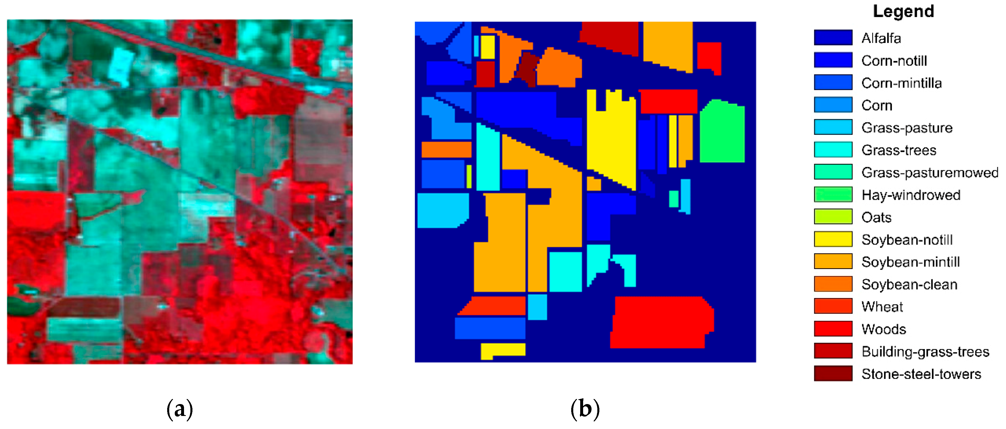
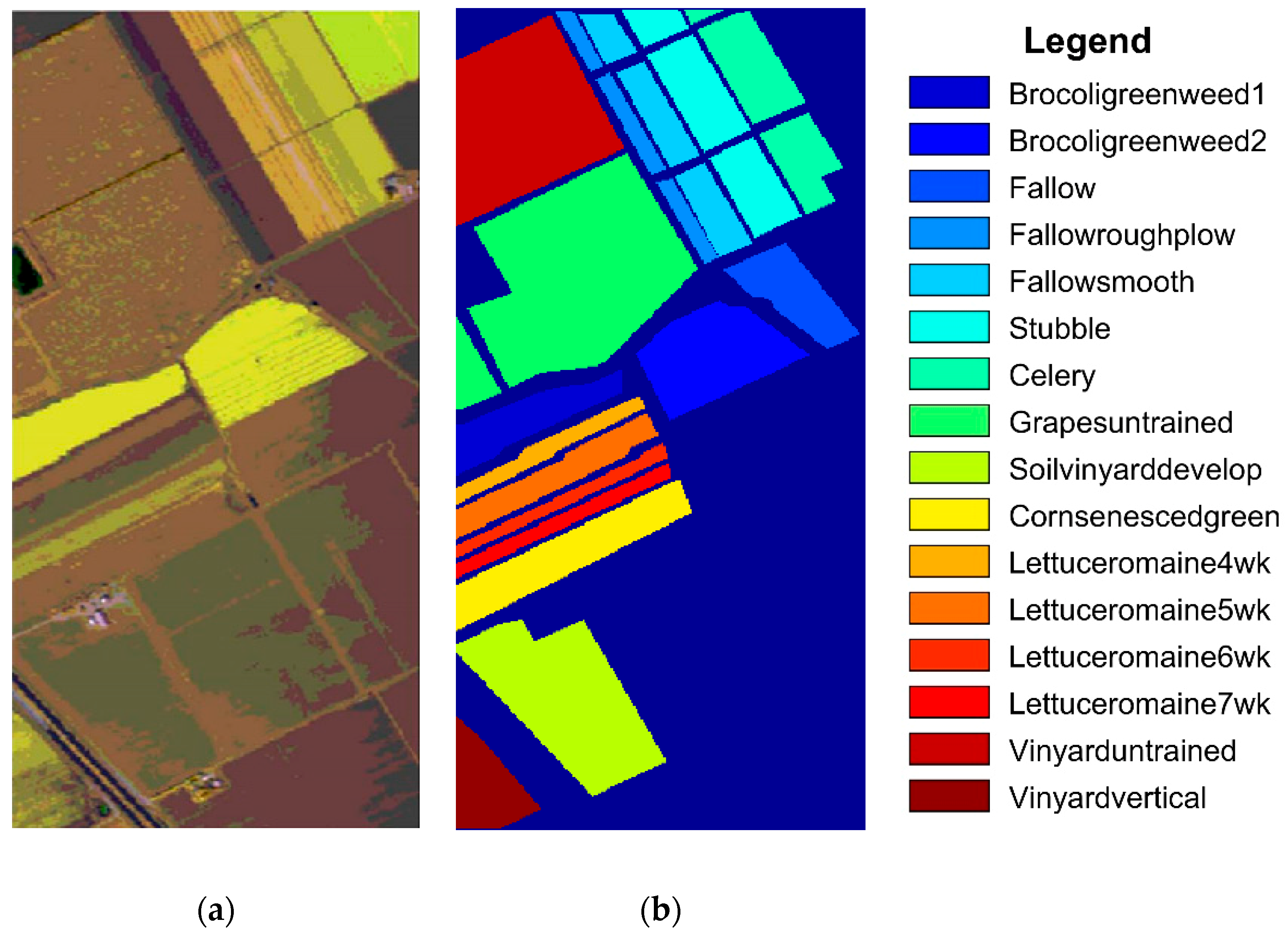
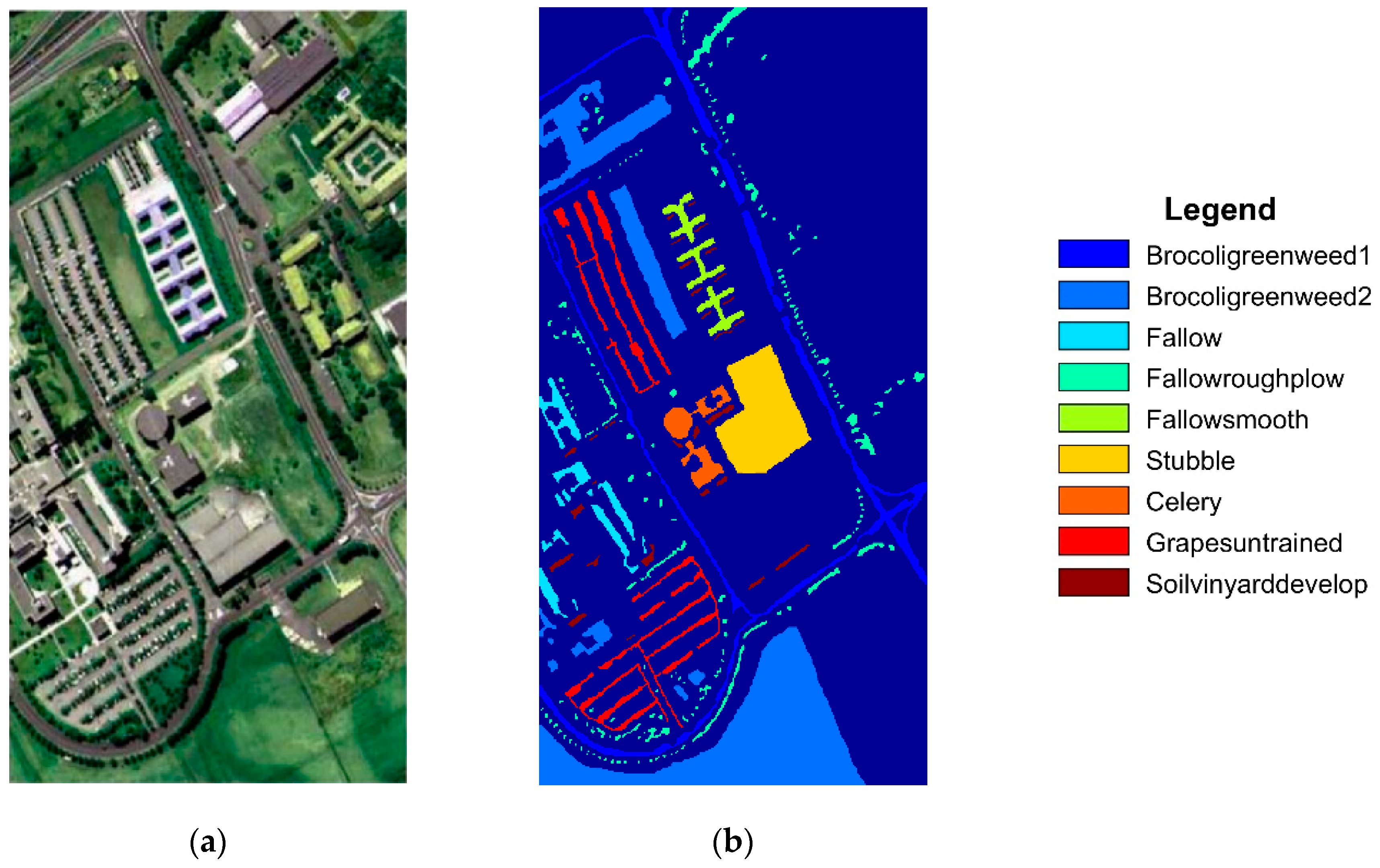
3.1. Hyperspectral Datasets

The main features and parameters of three benchmark hyperspectral datasets are described as follows.

A: Indian Pines dataset. This dataset was acquired by an airborne visible/infrared imaging spectrometer (AVIRIS) sensor over Indian Pines test site in the northwest of Indian. It consists of 145 × 145 pixels, 200 spectral bands, and 16 different classes. This HSI has a spatial resolution of 20 m. With the background removed, 10,249 pixels take part in the classification. Figure 1 shows the false-color image of Indian Pines dataset and the corresponding reference data.

B: Salinas dataset. This image was also captured by the AVIRIS sensor over Salinas Valley in California. This image is of size 512 × 217 × 204 (20 water absorption bands were discarded), which has a spatial resolution of 3.7 m. The provided data are divided into 16 classes. The false-color image of this dataset and the corresponding reference data are shown in Figure 2.

C: University of Pavia dataset. This image was collected by the reflective optics system imaging spectrometer (ROSIS) over University of Pavia in Italy. It contains nine classes and 103 bands after removing 12 noise bands. Each band size in this dataset is 610 × 340 with a spatial resolution of 1.3 m. The false-color image of this dataset and the corresponding reference data are shown in Figure 3.

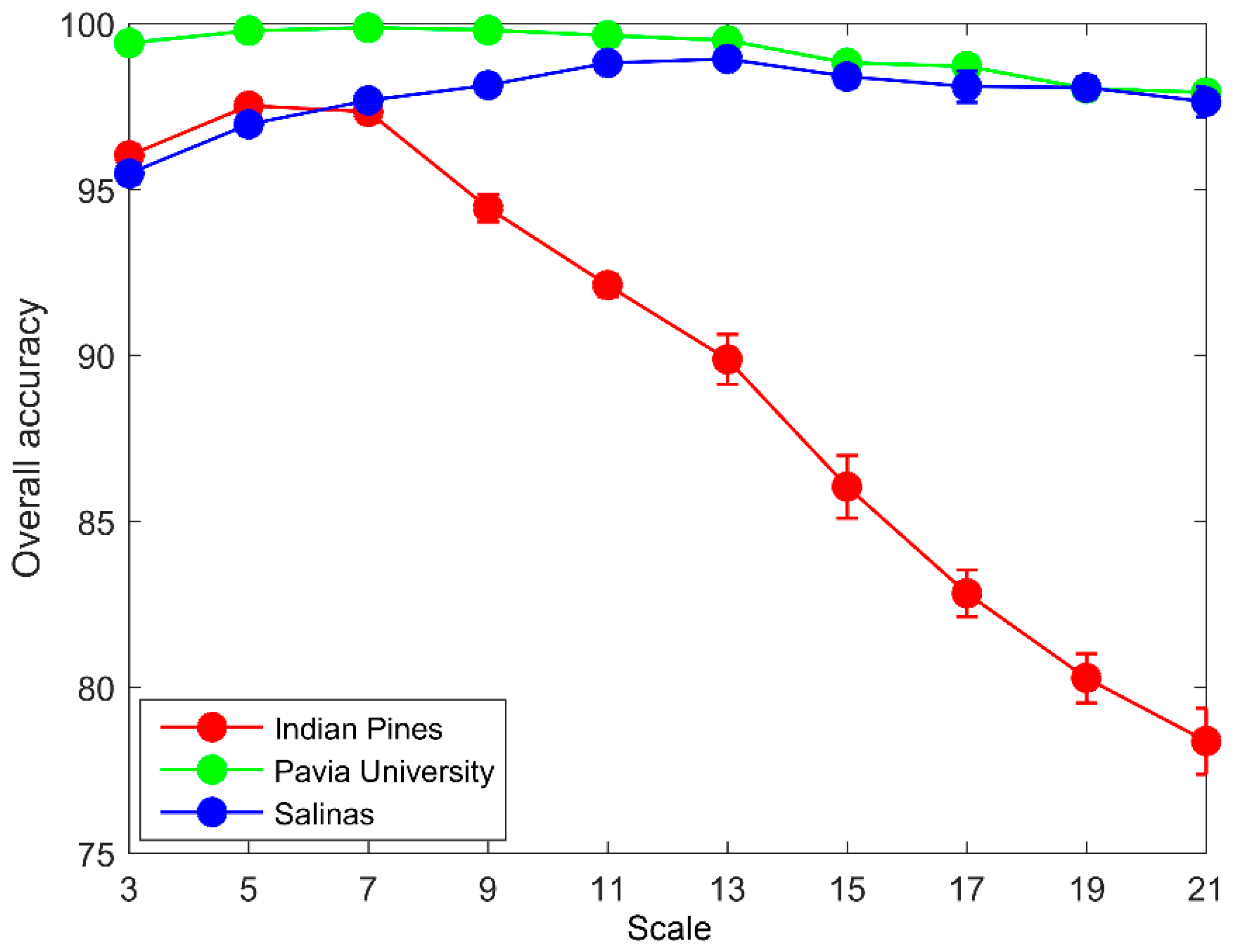
3.2. Impact of Segmentation Scale

In order to divide HSI into appropriate superpixels by using the improved SLIC algorithm, the segmentation scale needs to be pre-specified. The rise of segmentation scale means the increase of superpixel volume. Figure 4 shows that the classification accuracies of three datasets vary with the increase of segmentation scale s. For Indian Pines dataset, the best OA reaches 97.52% when s = 5; then the OA values drop sharply when s is greater than 7. In this dataset, the small volume of several classes, the spectral similarity between classes, and the spatial proximity of classes lead to the fact that a large superpixel likely contains different classes. As a result, the probability of misclassification for these superpixels increases greatly in the process of classification. The OA value on Salinas dataset shows a slow upward trend with the segmentation scale s varying from 3 to 13, and then decreases slowly. The reason is that superpixels with the right size can play a better role in denoising. Furthermore, high classification accuracy also explains the rationality of defined similarity between two superpixels. When the segmentation scale s is less than 13, the OA value of University of Pavia dataset is almost 100%. The reasons could be: (i) This dataset has a high spatial resolution; (ii) classes with similar spectral feature are not adjacent in space, for example, class Broccoligreenweed1 and class Broccoligreenweed2, as shown in Figure 3b. Superpixel technology is just good at dealing with this situation. For this dataset, we take s = 7 in our experiment. According to the above analysis, the classification results reported in the following subsection are obtained with a choice of the scales that is based on the reference ground truth that is not available in general.

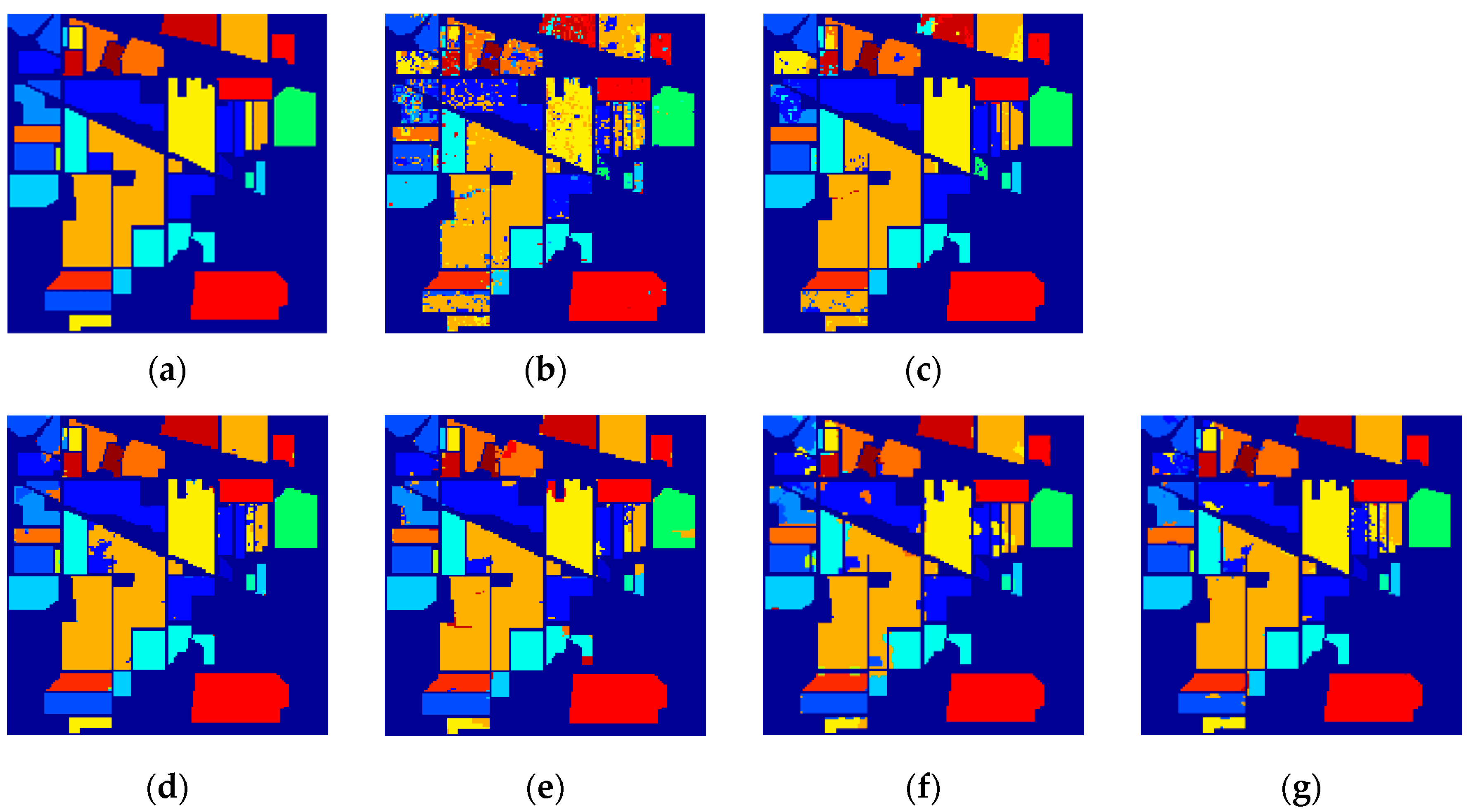
3.3. Classification Results

In

Table 1. The classification results on Indian Pines dataset achieved by SVM, EPF, IFRF, SuperPCA, PCA-SLIC, and the proposal SSB-SL.

Class	Train/Test	SVM	EPF	IFRF	SuperPCA	PCA-SLIC	SSC-SL
Alfalfa	5/41	49.76 ± 16.71	51.22 ± 40.17	94.63 ± 6.97	95.61 ± 1.54	100 ± 0	100.00 ± 0.00
Corn-notill	143/1285	67.87 ± 2.73	81.5 ± 4.22	91.27 ± 0.67	93.6 ± 2.34	95.86 ± 2.4	96.91 ± 2.53
Corn-mintilla	83/747	54.11 ± 2.2	60.48 ± 3.49	94 ± 2.84	95.57 ± 3.65	95.66 ± 3.4	96.13 ± 4.17
Corn	24/213	38.87 ± 7.74	66.95 ± 25.57	87.51 ± 6.59	87.23 ± 6.73	93.01 ± 7.57	93.21 ± 6.58
Grass-pasture	49/434	88.48 ± 2.99	94.45 ± 1.25	96.08 ± 1.73	95.83 ± 2.45	95.85 ± 3.19	96.17 ± 2.83
Grass-trees	73/657	96.41 ± 1.37	99.85 ± 0.16	99.09 ± 0.72	96.74 ± 2.76	97.42 ± 1.87	98.85 ± 0.35
Grass-pasturemowed	3/25	79.6 ± 7.65	96.8 ± 1.69	87.6 ± 14.78	96.4 ± 1.26	90.71 ± 6.9	93.57 ± 2.26
Hay-windrowed	48/430	97.37 ± 1.43	100 ± 0	100 ± 0	99.02 ± 1.79	99.79 ± 0.04	100.00 ± 0.00
Oats	2/18	26.67 ± 9.37	2.22 ± 7.03	15 ± 21.12	80 ± 25.82	100 ± 0	100.00 ± 0.00
Soybean-notill	98/874	65.94 ± 3.09	77.25 ± 2.74	89.99 ± 2.64	92.95 ± 2.66	93.37 ± 1	93.27 ± 2.71
Soybean-mintill	246/2209	84.83 ± 0.95	96.57 ± 0.83	98.47 ± 0.55	98.33 ± 1.35	97.76 ± 1.16	98.21 ± 1.06
Soybean-clean	60/533	64.43 ± 5.12	93.73 ± 8.21	90.51 ± 4.62	92.35 ± 2.56	94.2 ± 2.36	94.35 ± 2.82
Wheat	21/184	97.34 ± 2.15	99.3 ± 0.27	99.41 ± 0.17	97.39 ± 1.08	98.02 ± 1.87	98.69 ± 0.46
Woods	127/1138	96.57 ± 0.64	99.48 ± 0.43	99.68 ± 0.31	99.13 ± 0.88	98.62 ± 0.98	99.49 ± 0.38
Building-grass-trees	39/347	49.31 ± 7	73.31 ± 10.92	96.89 ± 1.94	91.96 ± 5.5	95.9 ± 3.01	96.61 ± 3.68
Stone-steel-towers	10/83	88.07 ± 4.66	99.28 ± 1.9	98.68 ± 1.33	83.73 ± 16.25	97.69 ± 5.19	97.74 ± 0.79
OA	--	77.63 ± 0.6	88.34 ± 1.1	95.49 ± 0.26	95.79 ± 0.51	96.61 ± 1.23	97.18 ± 1.26
AA	--	71.6 ± 4.74	80.77 ± 6.81	89.93 ± 4.19	93.49 ± 4.91	96.49 ± 2.28	97.07 ± 2.45
κ	--	0.7424 ± 0.69	0.8657 ± 1.28	0.9485 ± 0.3	0.9518 ± 0.59	0.960 ± 1.32	0.9649 ± 1.37

, the lowest classification accuracy (77.63%) is obtained by SVM because only the spectral features of pixels are used for classification in this method. In contrast, the classification accuracy of the EPF is improved by about 10% due to the application of spatial information. In particular, the classification accuracy provided by SSC-SL raises nearly 20%. The classification result of the superpixel-level SSC-SL is better than those of other three spectral–spatial methods PF, IFRF and SuperPCA. This indicates that the application of superpixel in classification is helpful to improve classification accuracy. The reason is that the superpixel-level classification method not only effectively merges the spectral and spatial information, but also has a good denoising effect on HSI. The classification result of PCA-SLIC on Oats shows that this method divides it into two or more superpixels, and there is always a misclassified superpixel. However, the improved SLIC algorithm can aggregate class Oats into a superpixel. The classification accuracy of 97.18% on Indian Pines dataset indicates that the introduced measurement, segmentation technique, and classification method are effective for unbalanced remote sensing datasets. Figure 5 presents the classification maps of these six methods on the Indian Pines dataset.

The statistical results of these six methods on Salinas dataset are shown in

Table 2. The classification results on the Salinas dataset provided by SVM, EPF, IFRF, SuperPCA, PCA-SLIC, and the proposal SSB-SL.

Class	Train/Test	SVM	EPF	IFRF	Super-PCA	PCA-SLIC	SSL-SL
Brocoligreenweed1	21/1988	97.64 ± 1.32	99.43 ± 0.63	100 ± 0	98.61 ± 4.39	100 ± 0	99.95 ± 0.01
Brocoligreenweed2	38/3688	98.81 ± 0.19	99.86 ± 0.08	99.34 ± 0.47	98 ± 2.86	99.7 ± 0	99.59 ± 0.32
Fallow	20/1956	84.92 ± 4.77	83.64 ± 5.08	99.95 ± 0.15	98.99 ± 0.2	99.59 ± 0.7	99.86 ± 0.13
Fallowroughplow	14/1380	98.96 ± 0.4	99.37 ± 0.34	96.63 ± 1.84	94.51 ± 4.95	89.45 ± 9.3	90.17 ± 8.6
Fallowsmooth	27/2651	97.26 ± 1.15	99.55 ± 0.28	99.27 ± 0.27	95.95 ± 5.8	97.26 ± 1.08	98.74 ± 0.26
Stubble	40/3919	99.56 ± 0.11	99.97 ± 0.02	99.92 ± 0.03	96 ± 5.1	99.92 ± 0	99.9 ± 0.01
Celery	36/3543	99.33 ± 0.25	99.74 ± 0.02	99.66 ± 0.2	96.64 ± 2.27	99.92 ± 0.02	99.92 ± 0.02
Grapesuntrained	113/11158	88.53 ± 2.05	91.35 ± 1.9	92.83 ± 0.81	97.74 ± 1.59	97.83 ± 1.18	99.1 ± 0.23
Soilvinyarddevelop	63/6140	98.54 ± 0.8	99.5 ± 0.32	99.98 ± 0	97.91 ± 3.54	99.89 ± 0.18	99.68 ± 0.29
Cornsenescedgreen	33/3245	87.34 ± 4.17	92.07 ± 3.35	99.67 ± 0.22	95.88 ± 2.2	95.33 ± 3.9	97.51 ± 0.62
Lettuceromaine 4wk	11/1057	90.67 ± 1.85	97.02 ± 1.38	90.59 ± 4.39	73.8 ± 22.74	94.4 ± 3.98	96.69 ± 4.25
Lettuceromaine 5wk	20/1907	99.76 ± 0.31	100 ± 0	100 ± 0.02	89.24 ± 8.71	95.11 ± 0.91	98.58 ± 1.06
Lettuceromaine 6wk	10/906	97.64 ± 0.61	97.79 ± 0.22	81.45 ± 2.9	92.41 ± 9.23	89.67 ± 6.89	97.39 ± 0.06
Lettuceromaine 7wk	11/1059	90.93 ± 4.02	94.24 ± 0.86	92.6 ± 1.32	83.9 ± 10.31	88.59 ± 6.91	95.75 ± 0.11
Vinyarduntrained	73/7195	55.39 ± 4.96	62.68 ± 5.37	93.97 ± 1.84	96.66 ± 3.92	94.98 ± 2.41	95.5 ± 1.8
Vinyardvertical	19/1788	95.35 ± 3.74	97.71 ± 1.87	98.98 ± 0.86	92.25 ± 4.77	98.66 ± 2.4	99.78 ± 0.01
OA	--	89.16 ± 0.68	91.68 ± 0.75	96.8 ± 0.27	95.90 ± 0.62	97.39 ± 0.56	98.41 ± 0.13
AA	--	92.54 ± 1.92	94.62 ± 1.36	96.55 ± 0.96	93.66 ± 5.8	96.27 ± 2.49	98.01 ± 1.1
κ	--	0.879 ± 0.76	0.9071 ± 0.85	0.9644 ± 0.3	0.9543 ± 0.69	0.9710 ± 0.63	0.9823 ± 0.15

. According to the OA index value, our algorithm achieves a better classification result of 99.03%. The classification result of EPF is slightly better than that of SVM in terms of OA (91.68% vs. 89.16%). It may be explained by the fact that the class boundaries of this dataset are relatively neat so that the advantage of EPF is not highlighted. The IFRF is superior to EPF and SuperPCA on this dataset. Part of the reason is that the transform domain recurrent filtering plays a good role in denoising in IFRF. It is easy to see from Table 2 that the classification accuracy of each class is greater than 95.5% in our classification result, except class Fallowroughplow (90.17%). It is worth noting that our method is still superior to the PCA-SLIC method without using balance parameters. Figure 6 shows the classification maps of these six methods on the Salinas dataset.

The University of Pavia dataset has the characteristic of good spatial separation of several classes with similar spectral feature, such as Fallow, Fallowroughplough and Fallowsmooth. There is no doubt that this characteristic not only reduces the possibility of misclassification of the pixels located near class boundary, but also enables the obtained superpixels to have a high purity. Therefore, as shown in

Table 3. The classification results on the University of Pavia dataset obtained by SVM, EPF, IFRF, SuperPCA, PCA-SLIC, and the proposal SSB-SL.

Class	Train/Test	SVM	EPF	IFRF	Super-PCA	PCA-SLIC	SSB-SL
Broccoligreenweed1	664/5967	91.68 ± 0.55	99.67 ± 0.21	98.42 ± 0.21	95.55 ± 0.46	99.6 ± 0.23	99.62 ± 0.2
Broccoligreenweed2	1865/16784	97.4 ± 0.3	99.94 ± 0.02	99.93 ± 0.05	99.3 ± 0.07	99.64 ± 0.22	99.77 ± 0.13
Fallow	210/1889	70.05 ± 2.22	72.32 ± 5.26	91.08 ± 4.18	95.74 ± 0.85	99.02 ± 0.53	97.98 ± 0.58
Fallowroughplough	307/2757	93.82 ± 0.95	98.23 ± 0.66	94.85 ± 0.86	83.71 ± 1.63	97.29 ± 0.75	97.36 ± 0.58
Fallowsmooth	135/1210	99.45 ± 0.18	99.93 ± 0.03	99.63 ± 0.18	91.23 ± 1.25	96.68 ± 2.17	99.78 ± 0.04
Stubble	503/4526	76.69 ± 1.25	94.21 ± 1.71	99.8 ± 0.07	98.21 ± 0.37	99.97 ± 0.04	99.8 ± 0.12
Celery	133/1197	82.87 ± 0.96	94.05 ± 1.2	98.52 ± 0.56	98.47 ± 0.42	99.92 ± 0	98.55 ± 0.93
Grapesuntrained	369/3313	88.37 ± 1.32	98.86 ± 0.3	89.36 ± 1.74	97.21 ± 0.36	99.23 ± 0.35	98.66 ± 0.38
Soilvineyarddevelop	95/852	98.88 ± 0.38	98.09 ± 0.63	57.56 ± 4.6	95.82 ± 0.79	99.25 ± 0.71	99.65 ± 0.11
OA	--	91.35 ± 0.18	97.43 ± 0.24	96.98 ± 0.19	95.03 ± 0.69	99.31 ± 0.09	99.35 ± 0.09
AA	--	88.8 ± 0.9	95.03 ± 1.11	92.13 ± 1.38	96.77 ± 0.17	98.96 ± 0.56	99.02 ± 0.34
κ	--	0.8844 ± 0.23	0.9658 ± 0.32	0.96 ± 0.26	0.957 ± 0.23	0.9913 ± 0.12	0.9915 ± 0.12

, all five spectral–spatial methods provide good classification results (greater than 95.03%). For two superpixel-based methods, SSC-SL and SuperPCA, the proposed method SSC-SL achieves better classification accuracy, which is higher of about 4% than SuperPCA (99.35% vs. 95.03%). Furthermore, the average accuracy of SSC-SL, 99.02%, also indicates that the proposed method can classify each class almost correctly. The characteristic of the class boundsary complexity of this dataset highlights the advantage of the EPF algorithm. This makes the classification results of EPF better than that of other two spectral–spatial methods of IFRF and SuperPCA. Figure 7 shows the classification maps of these six methods on University of Pavia dataset.

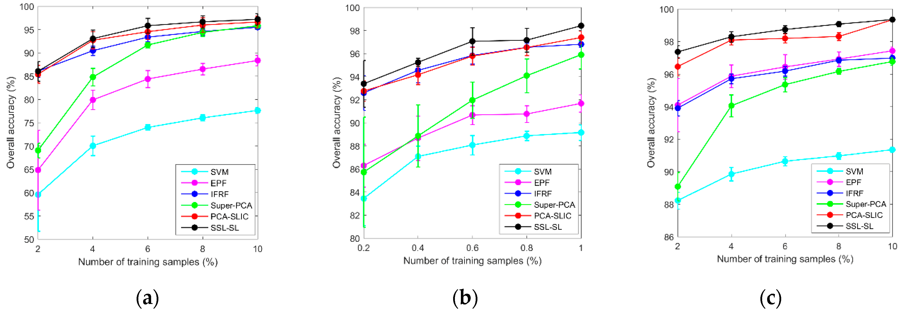
3.4. Effect of Different Numbers of Training Samples

The parameters used in EPF, IFRF, and SuperPCA are kept the same as original references. As shown in Figure 8, the classification accuracies of these six methods present an upward trend with the increase of label proportion on the three datasets. The proposed SSC-SL approach outperforms the other five compared methods for different label ratios of training samples on these three datasets. With the increase of label ratio, the strategy of randomly labeling pixels may not result in a significant increase of the number of labeled superpixels since it is possible to label more samples within a marked superpixel. In spite of this, the classifier we design still shows better classification performance. In particular, our classification result is about 3% better than that of EPF and IFRF on University of Pavia image in the case of marking limited samples (2%). The fact that SSC-SL is superior to PCA-SLIC on different datasets and for different label ratios, confirms the success and effectiveness of the improved SLIC algorithm.

4. Conclusions

In this work, we suggested an effective spectral–spatial classification method for HSI at superpixel level. The introduced similarity between two pixels effectively integrates the advantages of the correlation coefficient being sensitive to the spectra shape and the Euclidean distance being sensitive to spectra difference. In addition, the improved nonparametric SLIC algorithm can directly partition HSI with arbitrary dimensionality into superpixels. This facilitates its further application in the field of agricultural remote sensing. Furthermore, to better measure the similarity of a pair of superpixels defined, smaller weights are assigned to the noise pixels located in these two superpixels to weaken the influence of them on it. More important, the proposed superpixel-level classification framework has made a successful attempt to reduce the hyperspectral data volume. Experimental and comparative results on three real hyperspectral datasets confirm the validity of the proposed HSI classification method. Compared with three existing superpixel-level HSI classification approaches, the advantage of this method is simple to calculate and easy to understand. It means that the proposal is more likely to be applied in other remote sensing issues. In this work, the choice of the optimal segmentation scale is based on the experimental result. In the absence of a reference ground truth, it is worth to further solve this problem better. Moreover, we will also focus on the development of new spectral–spatial HSI classification method at superpixel level in the case of a limited number of training samples.

References

1. Lee, M.; Huang, Y.; Yao, H.; Thomson, S. Determining the effects of storage on cotton and soybean leaf samples for hyperspectral analysis. IEEE J. Sel. Top. Appl. Earth Obs. Remote Sens. 2014, 7, 2562–2570. [Google Scholar] [CrossRef]
2. Kanning, M.; Siegmann, B.; Jarmer, T. Regionalization of uncovered agricultural soils based on organic carbon and soil texture estimations. Remote Sens. 2016, 8, 927. [Google Scholar] [CrossRef] [Green Version]
3. Clark, M.L.; Roberts, D.A. Species-level differences in hyperspectral metrics among tropical rainforest trees as determined by a tree-based classifier. Remote Sens. 2012, 4, 1820–1855. [Google Scholar] [CrossRef] [Green Version]
4. Ryan, J.; Davis, C.; Tufillaro, N.; Kudela, R.; Gao, B. Application of the hyperspectral imager for the coastal ocean to phytoplankton ecology studies in Monterey Bay CA, USA. Remote Sens. 2014, 6, 1007–1025. [Google Scholar] [CrossRef] [Green Version]
5. Muller-Karger, F.; Roffer, M.; Walker, N.; Oliver, M. Satellite remote sensing in support of an integrated ocean observing system. IEEE Geosci. Remote Sens. Mag. 2013, 1, 8–18. [Google Scholar] [CrossRef]
6. Liu, Y.; Gao, G.; Gu, Y. Tensor matched subspace detector for hyperspectral target detection. IEEE Trans. Geosci. Remote Sens. 2017, 55, 1967–1974. [Google Scholar] [CrossRef]
7. Zhang, Y.; Du, B.; Zhang, L.; Liu, T. Joint sparse representation and multitask learning for hyperspectral target detection. IEEE Trans. Geosci. Remote Sens. 2017, 55, 894–906. [Google Scholar] [CrossRef]
8. Melgani, F.; Bruzzone, L. Classification of hyperspectral remote sensing images with support vector machines. IEEE Trans. Geosci. Remote Sens. 2004, 42, 1778–1790. [Google Scholar] [CrossRef] [Green Version]
9. Camps-Valls, G.; Bruzzone, L. Kernel-based methods for hyperspectral image classification. IEEE Trans. Geosci. Remote Sens. 2005, 43, 1351–1362. [Google Scholar] [CrossRef]
10. Li, J.; Bioucas-Dias, J.; Plaza, A. Semi-supervised hyperspectral image segmentation using multinomial logistic regression with active learning. IEEE Trans. Geosci. Remote Sens. 2010, 48, 4085–4098. [Google Scholar]
11. Ratle, F.; Camps-Valls, G.; Weston, J. Semi-supervised neural networks for efficient hyperspectral image classification. IEEE Trans. Geosci. Remote Sens. 2010, 48, 2271–2282. [Google Scholar] [CrossRef]
12. Rajan, S.; Ghosh, J.; Crawford, M. An active learning approach to hyperspectral data classification. IEEE Trans. Geosci. Remote Sens. 2008, 46, 1231–1242. [Google Scholar] [CrossRef]
13. Xia, J.; Ghamisi, P.; Yokoya, N.; Iwasaki, A. Random forest ensembles and extended multi-extinction profiles for hyperspectral image classification. IEEE Trans. Geosci. Remote Sens. 2018, 1, 202–216. [Google Scholar] [CrossRef] [Green Version]
14. Lu, T.; Li, S.; Fang, L.; Jia, X.; Benediktsson, J. From Subpixel to Superpixel: A Novel Fusion Framework for Hyperspectral Image Classification. IEEE Trans. Geosci. Remote Sens. 2017, 55, 4398–4411. [Google Scholar] [CrossRef]
15. Cao, X.; Xu, Z.; Meng, D. Spectral-Spatial Hyperspectral Image Classification via Robust Low-Rank Feature Extraction and Markov Random Field. Remote Sens. 2019, 11, 1565. [Google Scholar] [CrossRef] [Green Version]
16. Dong, C.; Naghedolfeizi, M.; Aberra, D.; Zeng, X. Spectral–Spatial Discriminant Feature Learning for Hyperspectral Image Classification. Remote Sens. 2019, 11, 1552. [Google Scholar] [CrossRef] [Green Version]
17. Ghamisi, P.; Mura, M.D.; Benediktsson, J. A survey on spectral-spatial classification techniques based on attribute profiles. IEEE Trans. Geos. Remote Sens. 2015, 53, 2335–2353. [Google Scholar] [CrossRef]
18. Li, J.; Xi, B.; Du, Q.; Song, R.; Li, Y.; Ren, G. Deep Kernel Extreme-Learning Machine for the Spectral-Spatial Classification of Hyperspectral Imagery. Remote Sens. 2018, 10, 2036. [Google Scholar] [CrossRef] [Green Version]
19. Feng, J.; Chen, J.; Liu, L.; Cao, X.; Zhang, X.; Jiao, L.; Yu, T. CNN-Based Multilayer Spatial-Spectral Feature Fusion and Sample Augmentation with Local and Nonlocal Constraints for Hyperspectral Image Classification. IEEE J. Sel. Top. Appl. Earth Obs. Remote Sens. 2019, 12, 1299–1313. [Google Scholar] [CrossRef]
20. Feng, J.; Yu, H.; Wang, L.; Cao, X.; Zhang, X.; Jiao, L. Classification of Hyperspectral Images Based on Multiclass Spatial-Spectral Generative Adversarial Networks. IEEE Trans. Geosci. Remote Sens. 2019, 57, 5329–5343. [Google Scholar] [CrossRef]
21. Liu, Y.; Shan, C.; Gao, Q.; Gao, X.; Han, J.; Cui, R. Hyperspectral image denoising via minimizing the partial sum of singular values and superpixel segmentation. Neurocomputing 2019. [Google Scholar] [CrossRef] [Green Version]
22. Jia, S.; Deng, B.; Zhu, J.; Jia, X.; Li, Q. Superpixel-Based Multitask Learning Framework for Hyperspectral Image Classification. IEEE Trans. Geosci. Remote Sens. 2017, 55, 2575–2588. [Google Scholar] [CrossRef]
23. Li, J.; Khodadadzadeh, M.; Plaza, A.; Jia, X.; Bioucas-Dias, J.M. A discontinuity preserving relaxation scheme for spectral–spatial hyperspectral image classification. IEEE J. Sel. Top. Appl. Earth Obs. Remote Sens. 2017, 9, 625–639. [Google Scholar] [CrossRef]
24. Dundar, T.; Ince, T. Sparse Representation-Based Hyperspectral Image Classification Using Multiscale Superpixels and Guided Filter. IEEE Trans. Geos. Remote Sens. Lett. 2018, 1–5. [Google Scholar] [CrossRef]
25. Fang, L.; Li, S.; Duan, W.; Ren, J.; Benediktsson, J.A. Classification of hyperspectral images by exploiting spectral–spatial information of superpixel via multiple kernels. IEEE Trans. Geosci. Remote Sens. 2015, 53, 6663–6674. [Google Scholar] [CrossRef] [Green Version]
26. Liu, T.; Gu, Y.; Chanussot, J.; Dalla Mura, M. Multimorphological Superpixel Model for Hyperspectral Image Classification. IEEE Trans. Geosci. Remote Sens. 2017, 55, 6950–6963. [Google Scholar] [CrossRef]
27. Zhang, L.; Su, H.; Shen, J. Hyperspectral Dimensionality Reduction Based on Multiscale Superpixelwise Kernel Principal Component Analysis. Remote Sens. 2019, 11, 1219. [Google Scholar] [CrossRef] [Green Version]
28. Xie, F.; Lei, C.; Yang, J.; Jin, C. An Effective Classification Scheme for Hyperspectral Image Based on Superpixel and Discontinuity Preserving Relaxation. Remote Sens. 2019, 11, 1149. [Google Scholar] [CrossRef] [Green Version]
29. Xue, Z.; Zhou, S.; Zhao, P. Active Learning Improved by Neighborhoods and Superpixels for Hyperspectral Image Classification. IEEE Geosci. Remote Sens. Lett. 2018, 99, 1–5. [Google Scholar] [CrossRef]
30. Liu, C.; Li, J.; He, L. Superpixel-Based Semisupervised Active Learning for Hyperspectral Image Classification. IEEE J. Sel. Top. Appl. Earth Obs. Remote Sens. 2019, 12, 357–370. [Google Scholar] [CrossRef]
31. Li, W.; Prasad, S.; Fowler, J.E. Hyperspectral image classification using gaussian mixture models and markov random fields. IEEE Trans. Geosci. Remote Sen Lett. 2013, 11, 153–157. [Google Scholar] [CrossRef] [Green Version]
32. Li, J.; Bioucas-Dias, J.M.; Plaza, A. Spectral-spatial hyperspectral image segmentation using subspace multinomial logistic regression and Markov random fields. IEEE Trans. Geosci. Remote Sens. 2012, 50, 809–823. [Google Scholar] [CrossRef]
33. Jia, S.; Deng, B.; Zhu, J.; Jia, X.; Li, Q. Local Binary Pattern-Based Hyperspectral Image Classification with Superpixel Guidance. IEEE Trans. Geosci. Remote Sens. 2018, 56, 749–759. [Google Scholar] [CrossRef]
34. Sun, H.; Ren, J.; Zhao, H.; Yan, Y.; Zabalza, J.; Marshall, S. Superpixel based Feature Specific Sparse Representation for Spectral-Spatial Classification of Hyperspectral Images. Remote Sens. 2019, 11, 536. [Google Scholar] [CrossRef] [Green Version]
35. Jiang, J.; Ma, J.; Chen, C.; Wang, Z.; Cai, Z.; Wang, L. SuperPCA: A Superpixelwise PCA Approach for Unsupervised Feature Extraction of Hyperspectral Imagery. IEEE Trans. Geosci. Remote Sens. 2018, 56, 4581–4593. [Google Scholar] [CrossRef] [Green Version]
36. Zhang, S.; Li, S.; Fu, W.; Fang, L. Multiscale Superpixel-Based Sparse Representation for Hyperspectral Image Classification. Remote Sens. 2017, 9, 139. [Google Scholar] [CrossRef] [Green Version]
37. Tarabalka, Y.; Benediktsson, J.; Chanussot, J.; Tilton, J. Multiple Spectral–Spatial Classification Approach for Hyperspectral Data. IEEE Trans. Geosci. Remote Sens. 2010, 48, 4122. [Google Scholar] [CrossRef]
38. Tan, K.; Li, E.; Du, Q.; Du, P. An efficient semi-supervised classification approach for hyperspectral imagery. ISPRS J. Photogramm. Remote Sens. 2014, 97, 36–45. [Google Scholar] [CrossRef]
39. Zu, B.; Xia, K.; Li, T.; He, Z.; Li, Y.; Hou, J.; Du, W. SLIC Superpixel-Based l2,1-Norm Robust Principal Component Analysis for Hyperspectral Image Classification. Sensors 2019, 19, 479. [Google Scholar] [CrossRef] [Green Version]
40. Lu, T.; Li, S.; Fang, L.; Bruzzone, L.; Benediktsson, J.A. Set-to-Set Distance-Based Spectral–Spatial Classification of Hyperspectral Images. IEEE Trans. Geosci. Remote Sens. 2016, 54, 1–13. [Google Scholar] [CrossRef]
41. Sellars, P.; Aviles-Rivero, A.; Schönlieb, C. Superpixel Contracted Graph-Based Learning for Hyperspectral Image Classification. arXiv 2019, arXiv:1903.06548v3. [Google Scholar]
42. Achanta, R.; Shaji, A.; Smith, K.; Lucchi, A.; Fua, P.; Süsstrunk, S. SLIC superpixels compared to state-of- the-art superpixel methods. IEEE Trans. Pattern Anal. Mach. Intell. 2012, 34, 2274–2282. [Google Scholar] [CrossRef] [PubMed] [Green Version]
43. Lu, T.; Wang, J.; Zhou, H.; Jiang, J.; Ma, J.; Wang, Z. Rectangular-Normalized Superpixel Entropy Index for Image Quality Assessment. Entropy 2018, 20, 947. [Google Scholar] [CrossRef] [Green Version]
44. Vincent, L.; Soille, P. Watersheds in digital spaces: An efficient algorithm based on immersion simulations. IEEE Trans. Pattern Anal. Mach. Intell. 1991, 13, 583–598. [Google Scholar] [CrossRef] [Green Version]
45. Comaniciu, D.; Meer, P. Mean shift: A robust approach toward feature space analysis. IEEE Trans. Pattern Anal. Mach. Intell. 2002, 24, 603–619. [Google Scholar] [CrossRef] [Green Version]
46. Levinshtein, A.; Stere, A.; Kutulakos, K.N.; Fleet, D.J.; Dickinson, S.J.; Siddiqi, K. Turbopixels: Fast superpixels using geometric flows. IEEE Trans. Pattern Anal. Mach. Intell. 2009, 31, 2290–2297. [Google Scholar] [CrossRef] [Green Version]
47. Tu, B.; Wang, J.; Kang, X.; Zhang, G.; Ou, X.; Guo, L. KNN-Based Representation of Superpixels for Hyperspectral Image Classification. IEEE J. Sel. Top. Appl. Earth Obs. Remote Sens. 2018, 11, 4032–4047. [Google Scholar] [CrossRef]
48. Gou, J.; Zhan, Y.; Rao, Y.; Shen, X.; Wang, X.; He, W. Improved pseudo nearest neighbor classification. Knowl. Based Syst. 2014, 70, 361–375. [Google Scholar] [CrossRef]
49. Cover, T.; Hart, P. Nearest neighbor pattern classification. IEEE Trans. Inform. Theory 1967, 13, 21–27. [Google Scholar] [CrossRef]
50. Mitani, Y.; Hamamoto, Y. A local mean-based nonparametric classifier. Pattern Recognit. Lett. 2006, 27, 1151–1159. [Google Scholar] [CrossRef]
51. Zeng, Y.; Yang, Y.; Zhao, L. Pseudo nearest neighbor rule for pattern classification. Expert Syst. Appl. 2009, 36, 3587–3595. [Google Scholar] [CrossRef]
52. Kang, X.; Li, S.; Benediktsson, J.A. Spectral–Spatial Hyperspectral Image Classification with Edge Preserving Filtering. IEEE Trans. Geosci. Remote Sens. 2014, 52, 2666–2677. [Google Scholar] [CrossRef]
53. Kang, X.; Li, S.; Benediktsson, J.A. Feature Extraction of Hyperspectral Images with Image Fusion and Recursive Filtering. IEEE Trans. Geosci. Remote Sens. 2014, 52, 3742–3752. [Google Scholar] [CrossRef]
Figure 1. Indian Pines dataset. (a) False color image. (b) Reference image.
Applsci 10 00463 g001
Figure 2. Salinas dataset. (a) False color image. (b) Reference image.
Applsci 10 00463 g002
Figure 3. University of Pavia dataset. (a) False color image. (b) Reference image.
Applsci 10 00463 g003
Figure 4. Overall accuracy of three datasets with variation of segmentation scale.
Applsci 10 00463 g004
Figure 5. The classification maps of these six methods on the Indian Pines dataset. (a) Reference image. (b) SVM. (c) EPF. (d) IFRF. (e) SuperPCA. (f) PCA-SLIC. (g) SSC-SL.
Applsci 10 00463 g005
Figure 6. The classification maps of these six methods on Salinas dataset. (a) Reference image. (b) SVM. (c) EPF. (d) IFRF. (e) SuperPCA. (f) PCA-SLIC. (g) SSC-SL.
Applsci 10 00463 g006
Figure 7. The classification maps of these six methods on the University of Pavia dataset. (a) Reference image. (b) SVM. (c) EPF. (d) IFRF. (e) SuperPCA. (f) PCA-SLIC. (g) SSC-SL.
Applsci 10 00463 g007
Figure 8. OA of six methods with different numbers of training samples on three datasets. (a) Indian Pines. (b) Salinas. (c) University of Pavia.
Applsci 10 00463 g008