Tool Wear Monitoring for Complex Part Milling Based on Deep Learning

Abstract

Tool wear monitoring is necessary for cost reduction and productivity improvement in the machining industry. Machine learning has been proven to be an effective means of tool wear monitoring. Feature engineering is the core of the machining learning model. In complex parts milling, cutting conditions are time-varying due to the variable engagement between cutting tool and the complex geometric features of the workpiece. In such cases, the features for accurate tool wear monitoring are tricky to select. Besides, usually few sensors are available in an actual machining situation. This causes a high correlation between the hand-designed features, leading to the low accuracy and weak generalization ability of the machine learning model. This paper presents a tool wear monitoring method for complex part milling based on deep learning. The features are pre-selected based on cutting force model and wavelet packet decomposition. The pre-selected cutting forces, cutting vibration and cutting condition features are input to a deep autoencoder for dimension reduction. Then, a deep multi-layer perceptron is developed to estimate the tool wear. The dataset is obtained with a carefully designed varying cutting depth milling experiment. The proposed method works well, with an error of 8.2% on testing samples, which shows an obvious advantage over the classic machine learning method.

1. Introduction

Tool wear is a cost driver in machining that affects quality and productivity and adds unscheduled downtime for tool changes and the reworking of damaged parts. Accurate tool wear monitoring is necessary to avoid these unnecessary costs. Tool wear monitoring methods can be categorized into two main groups: direct and indirect methods [1]. Direct methods measure the actual wear value with optical, laser or ultrasonic devices. Although direct methods measure tool wear precisely, they are difficult to implement in real-time machining because, in most cases, the tool wear area is unreachable due to the occlusion of workpiece structure and flood coolant. Indirect methods monitor in-process physical parameters to evaluate wear state, such as force, vibration, acoustic emission, current, power and temperature signals [2]. Nowadays, indirect methods are the most widely used in tool wear monitoring because they are easy to conduct in real time and can obtain acceptable accuracy by using a proper monitoring signals and modeling method.

Indirect tool wear monitoring methods can be divided into two categories: physical-based and data-driven methods. Physical-based methods first develop the hand-designed physical model, i.e., the mathematic relationship between tool wear and measurable physical quantities from the mechanism of machining, and then estimate tool wear value through monitoring signals based on the model. Choudhury and Rath [3] proposed an evaluating approach of milling tool flank wear based on the relationship between average tangential cutting force coefficients and tool wear. Cui [4] discussed the influences of process parameters, tool parameters, and tool wear on tangential cutting force coefficients in his dissertation. A recognition approach for milling tool wear was proposed, based on the relationship between tangential cutting force coefficients and tool wear. This approach was needed to solve the cutting force coefficients through actual cutting forces, and then the tool wear was recognized through the solved tangential cutting force coefficients. The complex calculations meant that the recognition speed was low, and the result was not precise enough. Shao et al. [5] established a cutting power model in face milling, which included the cutting conditions and the tool flank wear, and then proposed a tool wear monitoring approach based on this power model. Hou et al. [6] developed the relationship between flank wear and average milling force based on the stress distribution in the tool wear zone and applied this relationship to estimate the flank wear width in the milling process. Han et al. [7,8] proposed a mechanistic cutting force model considering various wear types for difficult-to-cut material drilling, which can be used for tool wear monitoring and process parameter optimization in the conditions of multiple tool wear existing on different cutting edges.

Due to the complexity of tool wear mechanism and randomness of the machining process, the physical-based monitoring methods are faced with the problem of low accuracy and weak universality [9,10]. In recent years, many data-driven tool wear monitoring methods have been proposed based on machine learning such as fuzzy logic, artificial neural network (ANN), support vector machine (SVM), and Bayesian networks. Yu [11] used logistic regression with penalization and manifold regularization for tool condition monitoring. Kilickap et al. [12] used ANN with the inputs of cutting speed, feed rate and depth of cut for tool wear prediction in the milling of Ti-6242S. Patra et al. [13] used ANN with thrust force signals for tool wear prediction in micro-drilling. Karam et al. [14] built an ANN-based cognitive decision-making system to extract signal features for online tool life prediction. In other studies, the ANNs with different inputs and architectures are employed to predict tool wear [15,16,17]. Madhusudana et al. [18] used SVM with the features extracted from discrete wavelet transformation in sound signals for tool condition monitoring in face milling. Benkedjouh et al. [19] used support vector regression (SVR) with the features extracted from multi-sensor signals to predict tool life. Zhang and Zhang [20] used a least-square SVM to develop a nonlinear regression model for tool wear prediction in the milling process. Yu et al. [21] proposed a weighted hidden Markov model for tool life prediction. Zhu and Liu [22] proposed a hidden semi-Markov model with dependent durations through cutting force signals for tool wear monitoring. Tobon-Mejia et al. [23] established a dynamic Bayesian network for tool condition monitoring and remaining useful life estimation. Kong et al. [24] proposed a Gaussian process regression model for tool wear prediction. Wu et al. [25] made a comparative study on different machining learning method including ANN, SVR and random forest for tool wear monitoring. Liu et al. [26] built an Elman_Adaboost predictor with Elman neural networks for milling tool wear assessment with several statistic features selected from multi-sensor data including spindle current, force, vibration and acoustic emission.

The accuracy and generalization ability of the above-mentioned conventional feature-based machining learning models are highly affected by the quality of the hand-designed features [27]. However, feature selection is problem-dependent and somewhat subjective in practice. Different from feature-based machining learning methods, deep learning can achieve adaptive feature learning, which is helpful to improve the adaptability of prediction methods. Moreover, layer-by-layer feature learning in deep network is more likely to learn essential features hidden in the monitoring data and then to improve prediction accuracy [28]. Common deep learning methods include deep multi-layer perceptron (DMLP), deep autoencoder (DAE), convolutional neural network (CNN) and long short-term memory (LSTM) network. Serin et al. [29] used DMLP neural networks to predict surface roughness and specific energy consumption during 5-axis milling. Ou et al. [30] proposed an online sequential extreme learning machine for tool wear state recognition with a stacked denoising autoencoder (SDAE) put forward to extract abstract features. Cao et al. [31] proposed a 2-D CNN for milling tool wear monitoring, with the spectrum of the high signal-to-noise ratio vibration signals obtained from the derived wavelet frames as input features. Aghazadeh et al. [32] employed a CNN with a hybrid feature extraction method using wavelet time-frequency transformation and spectral subtraction algorithms for tool wear estimation. Mart’ınez-Arellano et al. [33] built a CNN model with time series imaging technique to transform the input raw signals. Sun et al. [34] designed an LSTM network to predict multiple flank wear values using raw signals of cutting force, vibration and acoustic emission. Zhao et al. [35] used convolutional bi-directional LSTM networks for tool condition monitoring in milling process.

From the above, most existing deep learning methods use raw signals without feature pre-selection and hand-design to maximize the merits of deep learning. In the actual machining process, cutting conditions are strongly time-varying, especially for the milling of parts with complex geometry, of which the allowance and cutting depth drastically change along the whole tool path [36]. In most cases, in the actual machining environment, only a few types of monitoring signals are possible to acquire, and the input features from the signals are probably highly correlated, leading to low prediction accuracy and poor generalization ability in time-varying cutting conditions. Besides, the model based on the raw signal as input has weak interpretability and it is difficult to analyze the source of error.

To solve this problem, a tool wear monitoring method for complex part milling based on deep learning is proposed in this paper. Compared with the existing approaches, the features are pre-selected with cutting force model and wavelet packet decomposition. The cutting depth, cutting forces, cutting force coefficients and the energy of the cutting vibration are selected as the input parameters and the output is the flank wear. Then, a deep autoencoder is employed to retract the highly correlated features from the pre-selected features, followed by a deep neural network to predict the wear value. The dataset for training and testing of the deep learning model is obtained with a carefully designed varying depth milling experiment. The testing results prove the effectiveness of the proposed method.

The remainder of this paper is organized as follows. The proposed monitoring method based on deep learning is introduced in Section 2. The experiment is conducted in Section 3. The application and results of the proposed method are shown and discussed in Section 4. The conclusions are summarized in Section 5.

2. Method

2.1. Overall Monitoring Method

Tool wear monitoring usually uses force, vibration, acoustic emission, current, power and temperature signals. In this study, to accord with the situation of few sensors in real machining environment, cutting force is selected as the single signal used for tool wear monitoring. In complex part milling, the cutting depth usually varies with the profile of the part. In this case, the cutting force and stability are time-varying, and it is difficult to design features for accurate tool wear estimation. To address this problem, a feature extractor based on pre-selection and deep learning is developed. The hand-designed features from the cutting force signal are further extracted with a deep autoencoder and then input to the deep multi-layer perceptron to estimate the tool wear value. The framework of the proposed tool wear monitoring method is illustrated in Figure 1.

2.2. Feature Pre-Selection

The features are pre-selected from the cutting force signals as the input of the deep learning, including nine features, i.e., the radial cutting depth, the magnitudes of two cutting force components in the tangential and axial direction, four cutting force coefficients and the two cutting vibration features in the tangential and axial direction.

2.2.1. Cutting Force Features

Cutting force is the most sensitive quantity reflecting the changes in tool wear. The magnitudes of cutting forces are selected as the features for tool wear monitoring. Cutting force coefficients can also be used as the cutting condition independent features for tool wear monitoring in complex part milling. Thus, the cutting force coefficients are also selected as the features.

The cutting forces in the milling process are illustrated in Figure 2. The cutting force model can be expressed as

$$\{\begin{array}{l}{F}_{\mathrm{t}}\left(\varphi \right)=K_{\mathrm{tc}}bh\left(\varphi \right)+K_{\mathrm{te}}b\\ F_{\mathrm{r}}\left(\varphi \right)=K_{\mathrm{rc}}bh\left(\varphi \right)+K_{\mathrm{re}}b\\ F_{\mathrm{a}}\left(\varphi \right)=K_{\mathrm{ac}}bh\left(\varphi \right)+K_{\mathrm{ae}}b\end{array}$$

(1)

where $F_{\mathrm{t}}$, $F_{\mathrm{r}}$ and $F_{\mathrm{a}}$ are the tangential, radial and axial cutting force, $K_{\mathrm{tc}}$, $K_{\mathrm{rc}}$ and $K_{\mathrm{ac}}$ are the cutting force coefficients contributed by the shearing action in tangential, radial and axial directions, $K_{\mathrm{te}}$, $K_{\mathrm{re}}$ and $K_{\mathrm{ac}}$ are the edge constants, $\varphi$ is the instantaneous angle of immersion, $b$ is the edge contact length, $h$ is uncut chip thickness

$$h=f_z\sin \varphi$$

(2)

where $f_z$ is feedrate per tooth. According to Equations (1) and (2), the cutting force has a linear relationship with the uncut chip thickness $h$. When the spindle speed and feedrate are fixed, the uncut chip thickness $h$ changes with the sine of the instantaneous angle of immersion $\varphi$. The linear function can be rewritten as

$$\{\begin{array}{l}{F}_{\mathrm{t}}/b=K_{\mathrm{tc}}{f}_z\cdot \sin \varphi +K_{\mathrm{te}}\\ F_{\mathrm{r}}/b=K_{\mathrm{rc}}{f}_z\cdot \sin \varphi +K_{\mathrm{re}}\\ F_{\mathrm{a}}/b=K_{\mathrm{ac}}{f}_z\cdot \sin \varphi +K_{\mathrm{ae}}\end{array}$$

(3)

As per Equation (3), the cutting force coefficients can be calibrated by linear regression of the cutting force value. Let the slope and intercept of the linear function after linear fitting be $P_i$ and $Q_i$, respectively, the cutting force coefficients can be obtained as

$$\{\begin{array}{l}{K}_{\mathrm{ic}}=P_i/f_z\\ K_{\mathrm{ie}}=Q_i\end{array}$$

(4)

In complex part milling, the part is usually cut layer by layer in the axial direction. The tangential and radial force are varied significantly compared with the axial cutting force. Hence, in this study the average tangential and radial cutting forces $F_{\mathrm{t}}$, $F_{\mathrm{r}}$, and the tangential and radial cutting force coefficients $K_{\mathrm{tc}}$, $K_{\mathrm{rc}}$, $K_{\mathrm{te}}$, $K_{\mathrm{re}}$ are selected as the input features.

2.2.2. Cutting Vibration Features

Cutting vibration has high correlation with tool wear. In this study, the cutting vibration features are extracted from cutting force signals for tool wear monitoring. To this end, a three-layer wavelet packet decomposition is used to decompose the cutting force fluctuation components from the original cutting force signal, as shown in Figure 3.

Wavelet packet decomposition (WPD) is a time-frequency analysis method. In WPD, the scale function of a standard orthogonalization $\psi \left(x\right)$ is used, and with two scale difference recursive Equations, the orthogonal wavelet packet is generated as

$$\{\begin{array}{l}{w}_{2n}\left(x\right)=\sqrt{2}{\displaystyle {\sum }_{k=Z}{h}_k{w}_n\left(2x-k\right)}\\ w_{2n+1}\left(x\right)=\sqrt{2}{\displaystyle {\sum }_{k=Z}{g}_k{w}_n\left(2x-k\right)}\end{array}$$

(5)

where $w_0=\psi \left(x\right)$, $h_k$, $g_k$ are, respectively, a pair of conjugate quadrature filter coefficients derived from $\psi \left(x\right)$. For signal $s\left(t\right)$, the discrete orthogonal WPD is defined as the projection coefficient of $s\left(t\right)$ on the orthogonal wavelet packet base, which can be expressed as

$$P_s\left(n,j,k\right)=\langle s\left(t\right),w_{n,j,k}\left(t\right)\rangle ={\displaystyle \underset{-\infty }{\overset{+\infty }{\int }}s\left(t\right)\left[2^{-\frac{j}{2w_n}}\left(2^{-j}t-k\right)\right]dt}$$

(6)

where $\left\{P_s\left(n,j,k\right)\right\}$ is the WPD coefficient sequence of $s\left(t\right)$ on the orthogonal wavelet packet space $U_j^n$. By setting a group of different conjugate quadrature filter coefficients of $\left\{h_k\right\}$ and $\left\{g_k\right\}$, the wavelet packet transform coefficients can be expressed as

$$\{\begin{array}{l}{P}_s\left(2n,j,k\right)={\displaystyle {\sum }_{k=Z}{h}_{l-2k}{P}_s\left(n,j-1,l\right)}\\ P_s\left(2n+1,j,k\right)={\displaystyle {\sum }_{k=Z}{g}_{l-2k}{P}_s\left(n,j-1,l\right)}\end{array}$$

(7)

Then, the energy distribution of the reconstructed signal in the time-frequency domain is expressed as

$$E\left(j,n\right)={\displaystyle {\sum }_{k=Z}{\left[P_s\left(n,j,k\right)\right]}^2}$$

(8)

In this study, the reconstructed force component with WPD caused by vibration is adopted as the input feature for tool wear monitoring.

2.3. Deep Learning for Tool Wear Monitoring

2.3.1. Structure of the Deep Learning Network

The deep learning network for tool wear monitoring in variable cutting depth milling is shown in Figure 4. It consists of two parts, a deep autoencoder and a deep multi-layer perceptron. The deep autoencoder is used to reduce the dimension of the input vectors (the pre-selected features) and learn the highly correlated features. Then, the following deep multi-layer perceptron is used to learn the effect of the extracted features on the tool wear and predict the tool wear value.

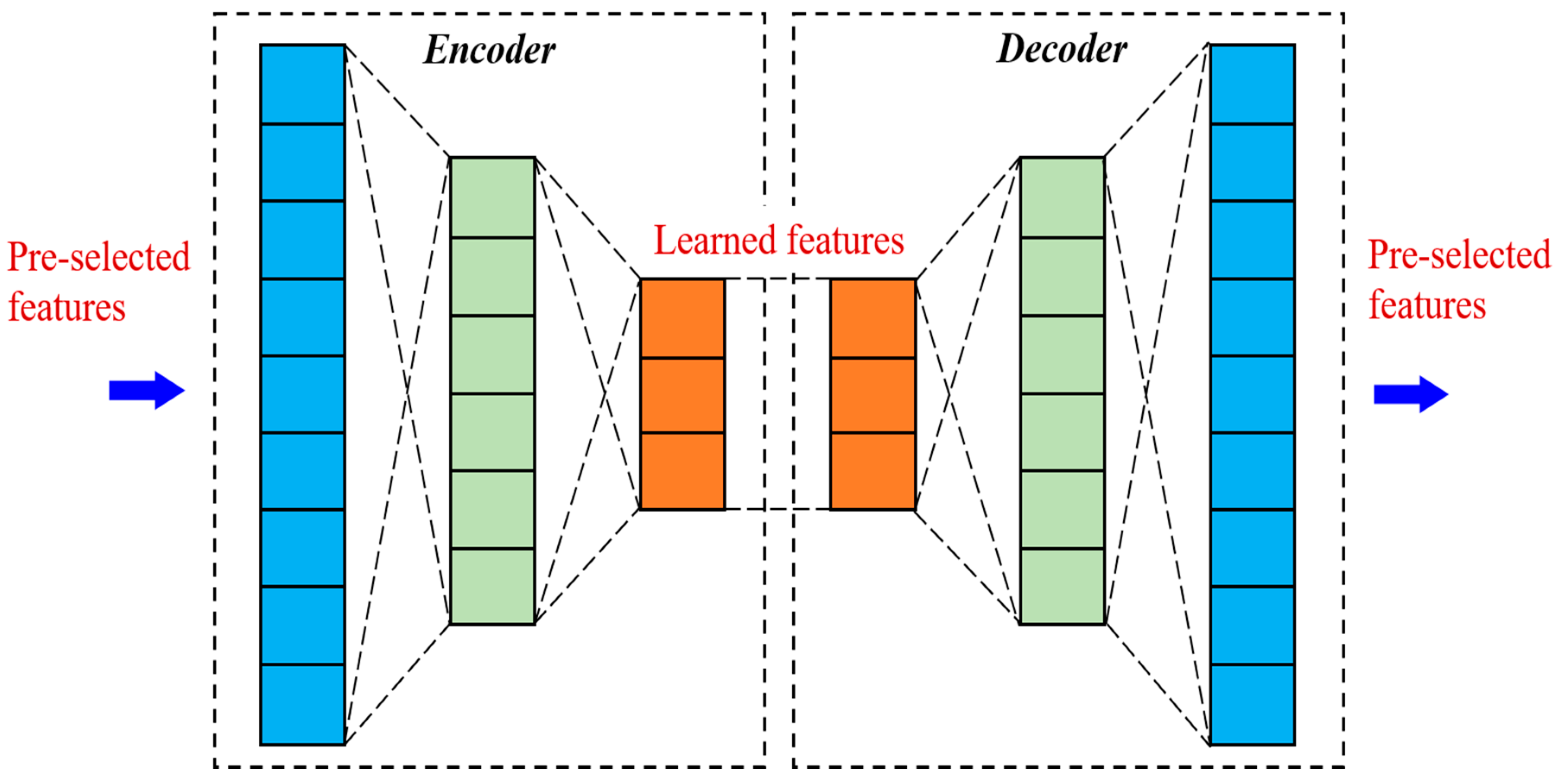
2.3.2. Deep Autoencoder

The pre-selected features are all obtained from cutting force signals. They are highly coupled and superfluous for tool wear prediction. This affects the accuracy and generalization ability of the deep learning model. In this study, the deep autoencoder (DAE) is used to learn the low-dimensional abstract features from the original features, which have a high correlation with the tool wear. The structure of the DAE is illustrated in Figure 5. Deep autoencoder is an unsupervised deep learning network for data dimensional reduction and feature extraction. It has a symmetric structure of multiple layers with the same input and output data. It consists of an encoder and a decoder. The transformation from the input layer to the middle hidden layer is called encoding. This is a dimensional reduction process, which transforms the high-dimensional original data into the low-dimensional space. The transformation from the middle hidden layer to the output layer is called decoding. This is the reconstruction process, which is the inverse of the encoder that reconstructs the encoded vector back to the original input data. In the encoding process, the obtained middle hidden layer reflects the essential features of the high-dimensional input data and is the core of the DAE. In this study, a six-layer DAE is developed with three layers for both the encoder and decoder.

The encoding process can be expressed as

$$h=f_{\theta }\left(x\right)=s_f\left(Wx+b\right)$$

(9)

The decoding process can be expressed as

$$\widehat{x}=g_{{\theta }^{\prime }}\left(h\right)=s_g\left(W^{\prime }h+b^{\prime }\right)$$

(10)

where $x={\left[x_1,x_2,\cdots ,x_n\right]}^T$ is the input vector, $h$ and $\widehat{x}={\left[{\widehat{x}}_1,{\widehat{x}}_2,\cdots ,{\widehat{x}}_n\right]}^T$ are the encoded and decoded vectors, $f_{\theta }$ and $g_{{\theta }^{\prime }}$ are the encoding and decoding functions, $W$ is the weight matrix from the input layer to the hidden layer, $W^{\prime }$ is the weight matrix from the hidden layer to the input layer, $b$ is the bias vector of the hidden layer, $b^{\prime }$ is the bias vector of the output layer, $\theta$ is the set of parameters in the encoding function, ${\theta }^{\prime }$ is the set of parameters in the decoding function, $s_f$ and $s_g$ are the activation functions of the encoder and decoder, which are both selected as the sigmoid function.

In the training process, to measure the error between the input $x$ and the reconstructed input $x^{\prime }$, the squared Euclidean distance is used as the loss function for this regression problem, which can be expressed as

$$Loss\left(W,b,W^{\prime },b^{\prime }\right)={\displaystyle \sum _{i=1}^n{\Vert x_i-{\widehat{x}}_i\Vert }^2}$$

(11)

After the DAE has been trained, the encoder (the first three layers) is employed as a feature extractor in front of the deep learning model.

2.3.3. Deep Multi-Layer Perceptron

The deep multi-layer perceptron is used to predict tool wear with the input of the extracted features from the DAE. The deep multi-layer perceptron consists of an input layer, a hidden layer and an output layer. The input layer and hidden layer are followed by a dropout layer. The number of neurons in each layer is tuned in the training process. The Rectified Linear Unit (ReLU) is used as the activation function, which can be expressed as

$$f\left(x\right)=\max \left(0,x\right)$$

(12)

2.3.4. Loss Function

The tool wear prediction is a regression problem. The target of network training is to minimize the error between the predicted and measured wear values. In this study, the mean squared error (MSE) is used to evaluate the prediction error, which can be expressed as

$$MSE=\frac{1}{n}{\displaystyle \sum _{i=1}^n{\Vert y_i-{\widehat{y}}_i\Vert }^2}$$

(13)

where $y={\left[y_1,y_2,\cdots ,y_n\right]}^T$ is the measured output vector which refers to the tool wear value, $\widehat{y}={\left[{\widehat{y}}_1,{\widehat{y}}_2,\cdots ,{\widehat{y}}_n\right]}^T$ is the predicted output vector, and $n$ is the number of samples.

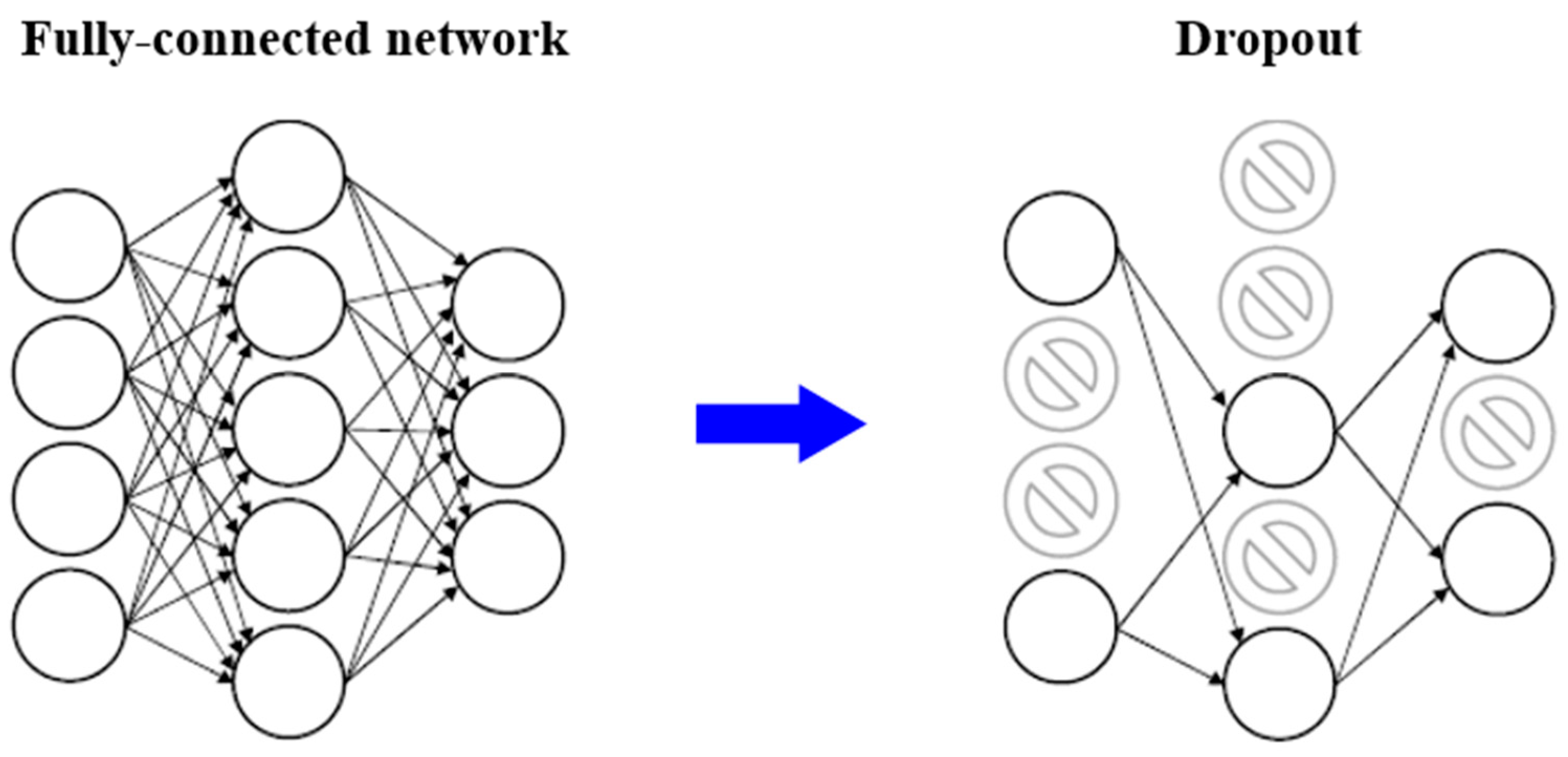
2.3.5. Regularization

Regularization is an effective technique used to enhance the generalization ability of deep neural network. The L1 and L2 regularization are generally used regularization methods. This involves adding the L1 norm or the L2 norm of the weight to the loss function in order to constrain the weight of the neural network. In this way, the networks with large weight values are abandoned in training process. In this study, to accord with the MSE loss value, L2 regularization is adopted. Then, the final loss function of the deep neural network can be expressed as

$$Loss=\frac{1}{n}{\displaystyle \sum _{i=1}^n{\Vert y_i-{\widehat{y}}_i\Vert }^2}+\frac{\lambda }{2}{\Vert w\Vert }^2$$

(14)

where $\Vert w\Vert$ is the L2 norm of the weight vector $w$, and $\lambda$ is the regularization parameter. The regularization parameter is tuned in the training process.

Another regularization approach is Dropout. In the Dropout method, the neurons in the network are deleted randomly in the training process, as illustrated in Figure 6. This trick can significantly reduce the interaction between the feature detectors (the hidden layer nodes). Detector interaction means that, in a deep network, some detectors only show their effect depending on other detectors. In this study, the dropout layers are inserted behind the input and hidden layers to diminish overfitting in training process. The dropout rate is set as 0.2, which means each neuron has a 20% probability of being deleted in the training process.

3. Experiment

To acquire the training and testing dataset for a deep learning model, the milling experiment is performed. The experimental setup is shown in Figure 7. The experiment is carried out on a YHVT850Z three-axis machining center. The work material is GH4169. The up milling is used with a 12 mm diameter indexable carbide insert tool APMT113PDER-H2. To control random factors in the machining process, the milling process is performed without a coolant. The cutting force is measured with a Kistler 9123C rotating dynamometer. The flank wear of the cutting tool was measured with Alicona InfiniteFocus optical measurement device.

To simulate the actual milling process with time-varying cutting depth, the milling process is designed with variable radial cutting depth. The tool path is illustrated in Figure 8. A total of 12 cutting passes are performed. For each pass, the radial cutting depth is from 0.5 to 1.5 mm. With the increase of cutting length, tool wear is gradually increased. Each cutting pass is divided into 10 segments. The cutting process was paused after each segment and the tool wear measurement was performed offline after each segment was finished. The average cutting forces in each segment are recorded as the input features of tool wear monitoring. The cutting parameters are listed in

Table 1. Cutting parameters in milling experiment.

Cutting Parameters	Setting Values
Spindle speed	1200 rev/min
Feedrate	0.05 mm/rev
Axial cutting depth	2 mm
Radial cutting depth	0.5~1.5 mm

.

4. Results and Discussion

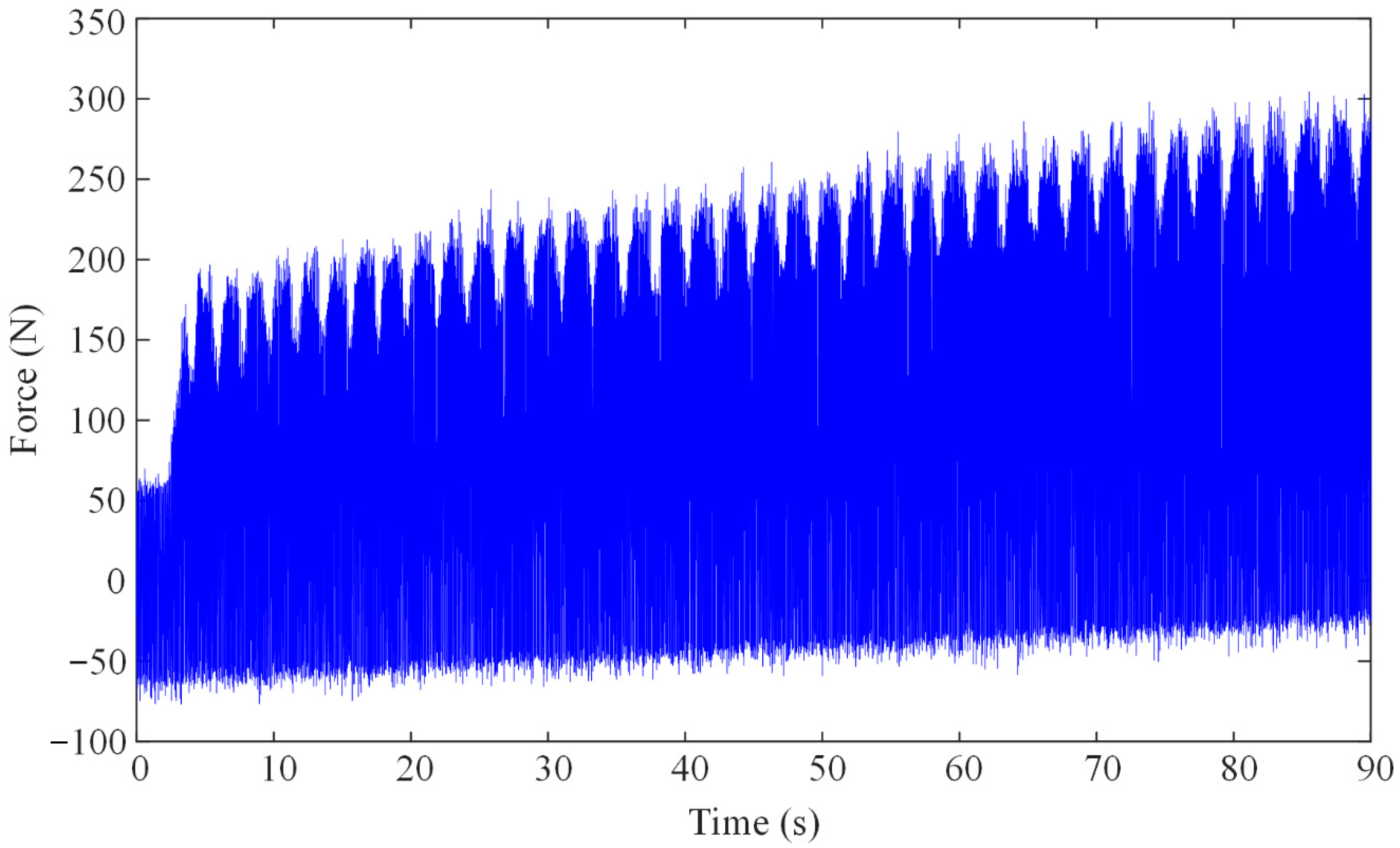
4.1. Features Extracted from Cutting Force Signals

The raw cutting force signal in a single segment is shown in Figure 9. This shows that the magnitude of the force is increased with the cutting depth. The average cutting force and the cutting force coefficients are selected as the input cutting force features of the deep learning model for tool wear monitoring. The average value of the cutting force in each segment are calculated and used as the input features. Cutting force coefficients are calibrated by applying linear regression as per Equations (3) and (4).

By reconstructing the cutting force signal with the WPD, the cutting force components caused by cutting vibration are obtained. The features related to tool wear are extracted from these two kinds of signals. With the three-layer WPD, the cutting force signals in the 0~1.5 KHZ are decomposed into eight frequency bands. By using 8 db wavelet packet decomposition, the width of each frequency band is 150 Hz. Taking the cutting force signal in three cycles as an example, the reconstructed signals in each band after WPD are shown in Figure 10.

From Figure 10, the reconstructed signals in different frequency band can be analyzed intuitively. According to the cutting force model Equation (1), the signal in the 0~150 Hz frequency band is related to the static cutting force component; the other signal in higher frequency band can be regarded as the dynamic component caused by cutting vibration and noise. From the results of WPD, the tangential force signal in 150~300 Hz is related to cutting vibration. The reconstructed force is denoted as $V_t$. The radial force signal in 450~600 Hz is related to cutting vibration. The reconstructed force is denoted as $V_r$. These two parameters are selected as the input cutting vibration features of the deep learning model for tool wear monitoring.

4.2. Training and Validation of Deep Neural Network

After the feature pre-selection and measurement shown above, the dataset for deep learning is shown in Appendix A. There are a total of 120 samples (acquired from 10 segments in 12 cutting passes). The Keras deep learning library is employed with Tensorflow as the back-end to implement the proposed deep learning networks. The dataset is randomly split into 80% training set (96 samples) and 20% testing set (24 samples). Before training, all the input parameters are normalized. Then, the grid search technique is employed to select the optimal hyper-parameters, including epochs, neuron numbers, optimizer, learning rate and regularization parameter. The obtained optimal hyper-parameters are given in

Table 2. Optimal hyper-parameters of deep neural network obtained by grid search.

Hyper-Parameters	Setting Values
Epochs	1000
Neuron number of the input layer	50
Neuron number of the hidden layer	10
Optimizer	RMSprop
Learning rate	0.001
Regularization parameter	0.001

.

With the proposed deep learning model in Section 2, with the above optimal hyper-parameters, the training process is carried out. In the training process, four-fold validation is used, with 24 samples in each fold. The mean value of the mean absolute error in all the fold is recorded as the training error.

The training curve is shown in Figure 11. The final mean absolute error after 1000 epochs is 34.93 μm, and the corresponding $R^2$ value is 0.9826. This proves the accuracy of the trained deep learning model.

The mean absolute error with the trained network in the four folds of the validation set is shown in Figure 12. The prediction error of tool wear value is less than 37 μm, and it is enough to monitor the tool wear state in the real machining process. This proves the effectiveness of the trained deep learning model.

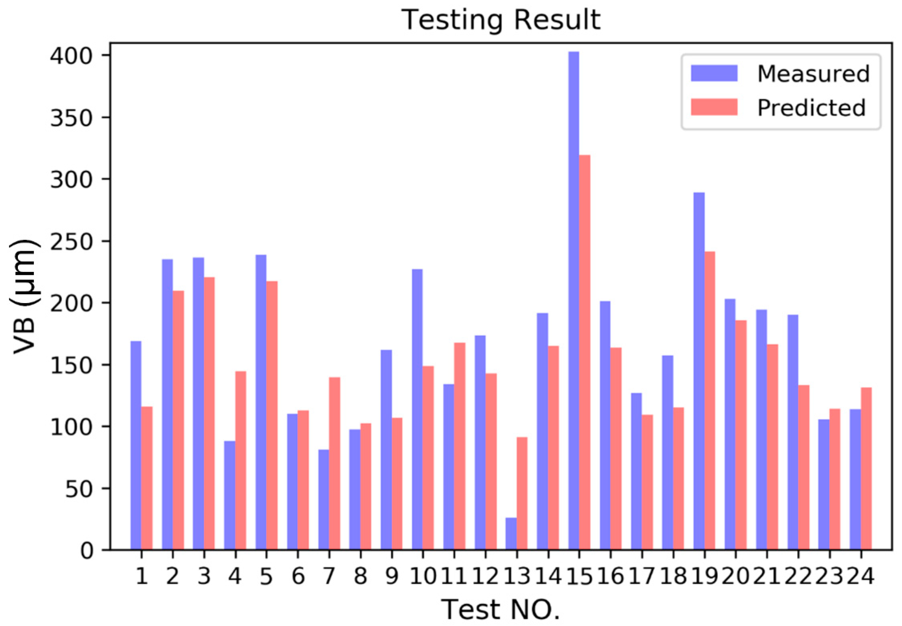
4.3. Testing of Deep Neural Network

The trained deep learning model is used for tool wear prediction on the testing set. The average error in percentage is used to evaluate the performance of the trained model, which is calculated as

$$error=\frac{1}{m}{\displaystyle \sum _{i=1}^m\frac{\left|V{B}_i^{*}-V{B}_i\right|}{V{B}_i}}$$

(15)

where $V{B}_i^{*}$ is the predicted tool wear value, $V{B}_i$ is the measured tool wear value, and $m$ is the total number of the testing samples.

The testing result is shown in Figure 13. The average error of the 24 testing samples is 8.2%, as per Equation (15). In the testing samples, the maximum relative error occurs in the test NO.13, with 64.8 μm larger than the measured value. In this case, the new tool has just begun to cut, with the measured flank wear of 25.7 μm. Besides, the maximum absolute error occurs in the test NO.15, with 82.3 μm less than the measured value. In this case, the cutting edge is seriously worn and the measured flank wear reaches 402.9 μm, far beyond the ISO tool wear criterion of 300 μm. Except for the two extreme cases shown above, where the actual tool wear value is too small or too large, the trained deep learning model predicts well for all the testing samples. For the cases where the tool wear is too small or too large, the model has a larger prediction error because the training set obtained from the experiment covers few samples of the tool wear with such extreme values, and thus the rules learnt in the model under these situations are somewhat under-fitting. The proposed deep learning model can be more accurate with more varied training data through additional experiments. This will be investigated in future research work. In this study, the testing result shows that the proposed model works well in most cases and this proves the generalization ability of the trained deep learning model.

Then, the radial basis function neural network (RBF NN) is implemented on the same dataset as the baseline to compare it with the performance of the proposed method. It turns out that the average error of RBF NN is 13.8%. Compared with the RBF NN, the proposed method shows higher accuracy in the tool wear prediction of varying cutting depth milling.

5. Conclusions

In this paper, a monitoring method based on deep learning is presented to give a solution to the feature extraction and accurate prediction of tool wear in complex part milling. A deep neural network is developed to estimate tool wear with the features pre-selected based on the cutting force model and wavelet packet decomposition, and further extracted using a deep autoencoder. The conclusions of this paper are summarized as: 1) the feature pre-selection based on cutting force model and wavelet packet decomposition and extraction coupled with a deep autoencoder is able to learn the highly correlated features for tool wear monitoring from single cutting force signals; 2) the proposed deep leaning model with the optimal settings has high accuracy for predicting tool wear; 3) the proposed deep learning method is proved to have higher accuracy than radial basis function neural network in varying cutting depth milling.

References

1. Liang, S.Y.; Hecker, R.L.; Landers, R.G. Machining process monitoring and control: The state-of-the-art. J. Manuf. Sci. Eng. 2004, 126, 297. [Google Scholar] [CrossRef]
2. Rehorn, A.G.; Jiang, J.; Orban, P.E. State-of-the-art methods and results in tool condition monitoring: A review. Int. J. Adv. Manuf. Technol. 2005, 26, 693–710. [Google Scholar] [CrossRef]
3. Choudhury, S.K.; Rath, S. In-process tool wear estimation in milling using cutting force model. J. Mater. Process. Technol. 2000, 99, 113–119. [Google Scholar] [CrossRef]
4. Cui, Y. Tool Wear Monitoring for Milling by Tracking Cutting Force Model Coefficients. Ph.D. Thesis, Shandong University, Jinan, China, 1997. [Google Scholar]
5. Shao, H.; Wang, H.L.; Zhao, X.M. A cutting power model for tool wear monitoring in milling. Int. J. Mach. Tools Manuf. 2004, 44, 1503–1509. [Google Scholar] [CrossRef]
6. Hou, Y.; Zhang, D.; Wu, B.; Luo, M. Milling Force Modeling of Worn Tool and Tool Flank Wear Recognition in End Milling. IEEE/ASME Trans. Mechatronics 2015, 20, 1024–1035. [Google Scholar] [CrossRef]
7. Han, C.; Luo, M.; Zhang, D.; Wu, B. Mechanistic modelling of worn drill cutting forces with drill wear effect coefficients. Procedia CIRP 2019, 82, 2–7. [Google Scholar] [CrossRef]
8. Han, C.; Luo, M.; Zhang, D. Optimization of varying-parameter drilling for multi-hole parts using metaheuristic algorithm coupled with self-adaptive penalty method. Appl. Soft Comput. 2020, 95, 106489. [Google Scholar] [CrossRef]
9. Han, C.; Zhang, D.; Luo, M.; Wu, B. Chip evacuation force modelling for deep hole drilling with twist drills. Int. J. Adv. Manuf. Technol. 2018, 98, 3091–3103. [Google Scholar] [CrossRef]
10. Han, C.; Luo, M.; Zhang, D.; Wu, B. Iterative Learning Method for Drilling Depth Optimization in Peck Deep-Hole Drilling. J. Manuf. Sci. Eng. 2018, 140, 121009. [Google Scholar] [CrossRef]
11. Yu, J. Tool condition prognostics using logistic regression with penalization and manifold regularization. Appl. Soft Comput. 2018, 64, 454–467. [Google Scholar] [CrossRef]
12. Kilickap, E.; Yardimeden, A.; Çelik, Y.H. Mathematical Modelling and Optimization of Cutting Force, Tool Wear and Surface Roughness by Using Artificial Neural Network and Response Surface Methodology in Milling of Ti-6242S. Appl. Sci. 2017, 7, 1064. [Google Scholar] [CrossRef] [Green Version]
13. Patra, K.; Jha, A.K.; Szalay, T.; Ranjan, J.; Monostori, L. Artificial neural network based tool condition monitoring in micro mechanical peck drilling using thrust force signals. Precis. Eng. 2017, 48, 279–291. [Google Scholar] [CrossRef]
14. Karam, S.; Centobelli, P.; D’Addona, D.M.; Teti, R. Online Prediction of Cutting Tool Life in Turning via Cognitive Decision Making. Procedia CIRP 2016, 41, 927–932. [Google Scholar] [CrossRef]
15. Venkatarao, K.; Murthy, B.; Rao, N.M. Prediction of cutting tool wear, surface roughness and vibration of work piece in boring of AISI 316 steel with artificial neural network. Measurement 2014, 51, 63–70. [Google Scholar] [CrossRef]
16. D’Addona, D.M.; Ullah, A.M.M.S.; Matarazzo, D. Tool-wear prediction and pattern-recognition using artificial neural network and DNA-based computing. J. Intell. Manuf. 2017, 28, 1285–1301. [Google Scholar] [CrossRef]
17. Mikołajczyk, T.; Nowicki, K.; Bustillo, A.; Pimenov, D.Y. Predicting tool life in turning operations using neural networks and image processing. Mech. Syst. Signal Process. 2018, 104, 503–513. [Google Scholar] [CrossRef]
18. Madhusudana, C.K.; Kumar, H.; Narendranath, S. Face milling tool condition monitoring using sound signal. Int. J. Syst. Assur. Eng. Manag. 2017, 8, 1643–1653. [Google Scholar] [CrossRef]
19. Benkedjouh, T.; Medjaher, K.; Zerhouni, N.; Rechak, S. Health assessment and life prediction of cutting tools based on support vector regression. J. Intell. Manuf. 2015, 26, 213–223. [Google Scholar] [CrossRef] [Green Version]
20. Zhang, C.; Zhang, H. Modelling and prediction of tool wear using LS-SVM in milling operation. Int. J. Comput. Integr. Manuf. 2016, 29, 76–91. [Google Scholar] [CrossRef]
21. Yu, J.; Liang, S.; Tang, D.; Liu, H. A weighted hidden Markov model approach for continuous-state tool wear monitoring and tool life prediction. Int. J. Adv. Manuf. Technol. 2017, 91, 201–211. [Google Scholar] [CrossRef]
22. Zhu, K.; Liu, T. Online Tool Wear Monitoring Via Hidden Semi-Markov Model with Dependent Durations. IEEE Trans. Ind. Inform. 2018, 14, 69–78. [Google Scholar] [CrossRef]
23. Tobon-Mejia, D.A.; Medjaher, K.; Zerhouni, N. CNC machine tool’s wear diagnostic and prognostic by using dynamic Bayesian networks. Mech. Syst. Signal Process. 2012, 28, 167–182. [Google Scholar] [CrossRef] [Green Version]
24. Kong, D.; Chen, Y.; Li, N. Gaussian process regression for tool wear prediction. Mech. Syst. Signal Process. 2018, 104, 556–574. [Google Scholar] [CrossRef]
25. Wu, D.; Jennings, C.; Terpenny, J.; Gao, R.X.; Kumara, S. A Comparative Study on Machine Learning Algorithms for Smart Manufacturing: Tool Wear Prediction Using Random Forests. J. Manuf. Sci. Eng. 2017, 139. [Google Scholar] [CrossRef]
26. Liu, Y.; Wang, F.; Lv, J.; Wang, X. A Novel Method for Tool Identification and Wear Condition Assessment Based on Multi-Sensor Data. Appl. Sci. 2020, 10, 2746. [Google Scholar] [CrossRef]
27. Serin, G.; Sener, B.; Ozbayoglu, A.M.; Unver, H.O. Review of tool condition monitoring in machining and opportunities for deep learning. Int. J. Adv. Manuf. Technol. 2020, 109, 953–974. [Google Scholar] [CrossRef]
28. Sun, C.; Ma, M.; Zhao, Z.; Tian, S.; Yan, R.; Chen, X. Deep Transfer Learning Based on Sparse Autoencoder for Remaining Useful Life Prediction of Tool in Manufacturing. IEEE Trans. Ind. Inform. 2019, 15, 2416–2425. [Google Scholar] [CrossRef]
29. Serin, G.; Gudelek, M.U.; Ozbayoglu, A.M.; Unver, H.O. Estimation of Parameters for the Free-Form Machining with Deep Neural Network. In Proceedings of the 2017 IEEE International Conference on Big Data (Big Data), Boston, MA, USA, 11–14 December 2017; IEEE: Piscataway, NJ, USA, 2017; pp. 2102–2111. [Google Scholar]
30. Ou, J.; Li, H.; Huang, G.; Yang, G. Intelligent Analysis of Tool Wear State Using Stacked Denoising Autoencoder with Online Sequential-Extreme Learning Machine. Measurement 2020, 108153. [Google Scholar] [CrossRef]
31. Cao, X.; Chen, B.; Yao, B.; Zhuang, S. An Intelligent Milling Tool Wear Monitoring Methodology Based on Convolutional Neural Network with Derived Wavelet Frames Coefficient. Appl. Sci. 2019, 9, 3912. [Google Scholar] [CrossRef] [Green Version]
32. Aghazadeh, F.; Tahan, A.; Thomas, M. Tool condition monitoring using spectral subtraction and convolutional neural networks in milling process. Int. J. Adv. Manuf. Technol. 2018, 98, 3217–3227. [Google Scholar] [CrossRef]
33. Martínez-Arellano, G.; Terrazas, G.; Ratchev, S. Tool wear classification using time series imaging and deep learning. Int. J. Adv. Manuf. Technol. 2019, 104, 3647–3662. [Google Scholar] [CrossRef] [Green Version]
34. Sun, H.; Zhang, J.; Mo, R.; Zhang, X. In-process tool condition forecasting based on a deep learning method. Robot. Cim. Int. Manuf. 2020, 64, 101924. [Google Scholar] [CrossRef]
35. Zhao, R.; Yan, R.; Wang, J.; Mao, K. Learning to Monitor Machine Health with Convolutional Bi-Directional LSTM Networks. Sensors 2017, 17, 273. [Google Scholar] [CrossRef] [PubMed]
36. Han, C.; Zhang, D.; Wu, B.; Pu, K.; Luo, M. Localization of freeform surface workpiece with particle swarm optimization algorithm. In Proceedings of the 2014 International Conference on Innovative Design and Manufacturing (ICIDM), Montreal, QC, Canada, 13–15 August 2014; IEEE: Piscataway, NJ, USA, 2014; pp. 47–52. [Google Scholar]
Figure 1. Framework of tool wear monitoring method for complex part milling based on deep learning.
Applsci 10 06916 g001
Figure 2. Interaction of tool and workpiece in milling process.
Applsci 10 06916 g002
Figure 3. Structure of the three-layer wavelet packet decomposition for reconstruction of cutting force signals.
Applsci 10 06916 g003
Figure 4. Architecture of deep learning network for tool wear prediction combining autoencoder and multi-layer perceptron.
Applsci 10 06916 g004
Figure 5. Symmetrical structure of deep autoencoder consisting of three-layer encoder and three-layer decoder.
Applsci 10 06916 g005
Figure 6. Schematic representation of dropout trick in a fully connected network.
Applsci 10 06916 g006
Figure 7. Experimental setup: (a) cutting force online measurement system, (b) layout of cutting tool and workpiece.
Applsci 10 06916 g007
Figure 8. Tool path of varying depth milling: (a) tool path design, (b) tool path, (c) cutting process simulation.
Applsci 10 06916 g008
Figure 9. Raw signal of cutting force in a single segment.
Applsci 10 06916 g009
Figure 10. Reconstructed cutting force signals in each frequency band with wavelet packet decomposition.
Applsci 10 06916 g010
Figure 11. Mean absolute error of proposed deep learning model in training process.
Applsci 10 06916 g011
Figure 12. Mean absolute error in four-fold validation set.
Applsci 10 06916 g012
Figure 13. Testing result in 24 samples of the trained deep learning model.
Applsci 10 06916 g013