Semi-Active Magnetorheological Damper Device for Chatter Mitigation during Milling of Thin-Floor Components

Abstract

The productivity during the machining of thin-floor components is limited due to unstable vibrations, which lead to poor surface quality and part rejection at the last stage of the manufacturing process. In this article, a semi-active magnetorheological damper device is designed in order to suppress chatter conditions during the milling operations of thin-floor components. To validate the performance of the magnetorheological (MR) damper device, a 1 degree of freedom experimental setup was designed to mimic the machining of thin-floor components and then, the stability boundaries were computed using the Enhance Multistage Homotopy Perturbation Method (EMHPM) together with a novel cutting force model in which the bull-nose end mill is discretized in disks. It was found that the predicted EMHPM stability lobes of the cantilever beam closely follow experimental data. The end of the paper shows that the usage of the MR damper device modifies the stability boundaries with a productivity increase by a factor of at least 3.

1. Introduction

The manufacturing of parts such as impellers, ribs, blisks, and turbine blades among other components for the aerospace industry requires the machining of thin-wall and thin-floor features [1]. Titanium, aluminum alloys, and superalloys such as Inconel are used for these applications because of their good corrosion resistance, lightweight, and mechanical properties. Most of these components are machined as monolithic parts to improve their performance and their weight-resistant ratio. However, the lightweight design of these components has as a consequence thin walls and thin floors to achieve a good buy-to-fly ratio [2]. The low stiffness at specific part locations makes machining prone to unstable regenerative vibrations (chatter), which is detrimental during finishing machining operations, causing negative effects on surface quality and tool life. To avoid vibration, chip load and cutting forces are kept in conservative values, resulting in decreasing productivity. Therefore, the machining of monolithic parts represents a great technological challenge that is faced with several off-line and in-line solutions.

Literature offers in-line solutions from fixing perspectives [3], workpiece holders [4], stiffening devices [5], and active materials [6]. In fact, the use of these materials such as piezoelectric, magnetostrictive, magnetorheological (MR), and electrorheological (RT) materials has been implemented in actuators and sensors devices in manufacturing applications.

Among the active materials, also called smart materials, the MR and RT materials whose rheological behavior can be controlled externally through a magnetic and electrical field are mainly used as damper and spring devices. The MR fluids have a vast range of applications in different areas such as the automotive industry and civil engineering. For instance, the automotive industry has developed semi-active damper devices for automotive suspension, together with the control of the systems [7]. In civil engineering, MR damper devices are used to change the structural behavior of buildings during earthquakes [8]. In addition, the use of MR fluids is extended in several areas of engineering such as the research of vibrations of pipelines reported by Hui et al. [9]. Concisely, MR technology supports many applications over different industrial contexts.

In machining, it is a common practice to instrument MR and RT materials in the clamping systems so that workpiece properties can be modified by adjusting their damping and stiffness [10]. The MR and RT fluids can work at a wide frequency range; their response occurs in a short time and offers flexibility to be adapted to different machining processes. Recently, in [11], Fleischer et al. studied some industrial applications of this technology; however, the use of these smart materials in machining processes has evolved because of their feasibility of being implemented for scale-up production.

Segalman and Redmond [12] used ER fluids for chatter suppression; they applied a cyclic electrical field to the spindle quill, changing the natural frequency of the spindle, which disrupts the modulation of tool vibrations. They found significant reductions in vibration amplitudes through simulation of the milling process. Wang and Fei [13] used an ER fluid-filled sleeve to increase the stiffness and damping of a boring bar. They concluded that the applied electric field strength should be adjusted on-line according to the detected vibration signals. Mei et al. [14] used MR fluids to mitigate chatter on a boring bar by adjusting the bar stiffness via a magnetic field intensity. Similarly, Çeşmesi and Engin [15] developed an MR damper device that was implemented in a conventional impact machine. Their mathematical model was able to predict the behavior of the damper device by controlling the magnetic field. According to Som et al. [16], the attenuation rate of the semi-active MR actuator in a boring process can be up to 30% in wide frequency ranges of 400 to 600 Hz. Furthermore, MR devices have the capability of substantially improving surface finish and reducing tool wear in hard-turning operations [17]. The design of the MR damper device can be assisted by Finite Element Method simulation because it can identify the magnetic field magnitudes needed when located in a tool-holder [18]. It is interesting to point out that most implementations of MR damper devices in machining operations were mainly oriented to boring or turning operations. This could be explained since the MR damper devices could be easily attached to the tool-holder in lathe machines. However, its implementation in milling operations is very infrequent, but there have been a few attempts to apply MR technology to increase the damping of the workpiece. For instance, Ma et al. [19] demonstrated stability improvement in the thin-wall milling process.

The most common off-line approach is focused on the calculation of chatter-free cutting parameters based on the study of dynamics stability [20]. Special milling tools such as spherical or bull-nose tools are preferred for thin-floor machining in order to obtain a certain curvature between floors and walls; however, the geometry of the cutting edge has a strong influence over the forces in the tool axis direction, which typically coincides with the direction of the low-dynamic stiffness of thin floors. Since thin-floor dynamics are inherently complex due to the modal parameter variation that depends on the tool-workpiece location, three-dimensional stability diagrams for bull-nose milling tool cutting operations were calculated for identification of the location at which the spindle speed of the cutting tool is a chatter-free tuning interval value [21]. Of course, the accuracy of the location of stability zones depends on predicting the magnitude values of cutting forces. In this sense, Budak et al. [22] developed a method to predict the cutting force of any cutter geometry from orthogonal cutting data. The accuracy of the predicted forces was assessed with collected experimental data. The same method was also applied to ball-end milling tools [23]. By fitting pressure and friction coefficients on the rake and flank contact surfaces of ball cutters, Yucesan et al. [24] predicted with good accuracy the acting cutting forces in Cartesian directions.

Altintas [25] described the chip regeneration mechanism in three directions with a bull nose. The stability lobes were predicted in the frequency domain and verified experimentally. Other methods to predict stability are based on the time-domain discretization. For instance, Olvera et al. [26] proposed the Enhanced Multistage Homotopy Perturbation Method to compute stability lobes in one degree of freedom mimicking thin wall machining. Later, Urbikain et al. [27] proposed stability colormaps based on time-domain simulations of peripheral milling in thin-walled parts with barrel cutters. Regarding tool path planning in thin floors, Smith and Dvorak [28] proposed a tool path strategy that provided extra stiffness by leftover material in the corners; however, this strategy is limited for large areas consisting of mostly thin floors.

To implement reliable solutions for the machining operations of thin-floor components, two aspects need to be considered. Firstly, high accuracy is required for the determination of the modal parameters and the associated acting cutting forces for effective and reliable stability prediction. Secondly, it is important to acknowledge the shortcomings of active or semi-active damping techniques, including excessive setup times and customized designs that are only suitable for some specific machine processes. The use of MR fluids still is not mature in cutting operations and requires more investigation if one wants to enhance its industrial application.

Therefore, the aim of this work focuses on investigating how a semi-active MR damping device can influence the dynamics of cutting operations in thin-floor components. First, a stability prediction model is developed, and its accuracy is assessed by considering the milling operations of a thin-floor component with bull-end mills. Second, a semi-active damping device based on MR fluid is designed for improving chatter-free cutting conditions to increase productivity. In this sense, the proposed damper device is studied experimentally in order to improve the stability lobes for thin-floor machining operations.

This paper is summarized as follows. Section 2 focuses on developing the cutting force model for a bull-nose milling tool based on variable cutting coefficients. Section 3 describes the method used to compute the stability analysis in thin-floor machining and comparing theoretical prediction with experimental data. Section 4 describes the development of a semi-active MR damper device that is an influence on thin-floor dynamics to increase stability lobes and productivity. Finally, some conclusions are drawn.

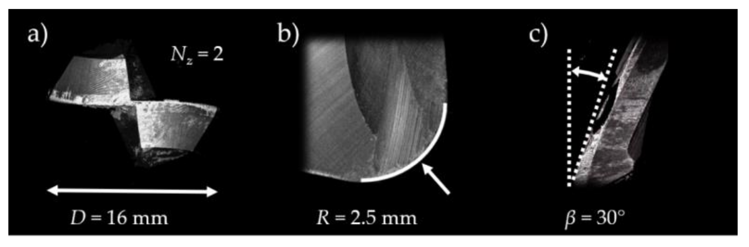
2. A Mechanistic Model for Bull-Nose End Mills

The cutting forces in a flat end milling are dominant in the x− and y− directions. However, for ball and bull-nose end milling, the cutting forces have significant components in all three Cartesian directions [25,29,30]. For chatter analysis of thin floors using bull-nose end milling, the accuracy of the cutting force models is critical to predict reliable stability lobes. The semi-empirical models are based on the assumption that the cutting forces and the undeformed chip section are linked through the cutting coefficients. The shear coefficient represents the amount of force required for a tool to remove an uncut chip, while the edge coefficient is related to the friction forces.

A bull-nose end milling tool with a tool diameter D, helix angle β, and tooth N_z, is defined by corner radius R (also called the ball radius). The bull-nose end mill used was purchased from 3G tool supplier and the main geometry characteristics described earlier were measured with an Alicona microscope model InfiniteFocusG5 (Alicona Imaging GmbH, Pforzheim, Germany) together with a 2.5X objective. As illustrated in Figure 1, optical microscope photographs confirm a tool diameter of 16 mm and a nose radius of 2.5 mm.

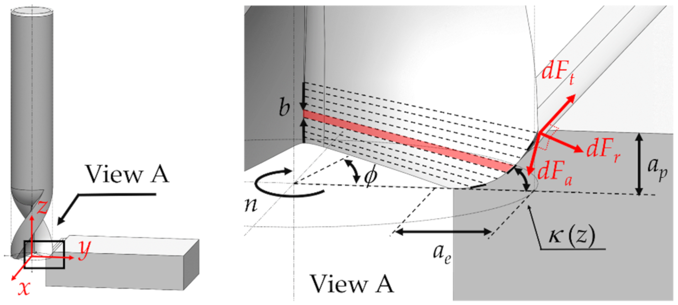
2.1. Cutting Force Model

A force model was developed to obtain an instantaneous cutting force magnitude for a given depth of cut. It is based on a mechanistic approach that assumes a relationship between forces and the uncut chip thickness by means of the cutting coefficients. Cutting models have been developed for ball-end mills that present similarities with the geometry of a bull-nose end mill. For instance, Yucesan et al. [24] proposed a model based on an analytic representation of ball-shaped helical flute geometry. Budak et al. reported the prediction of forces from the orthogonal cutting data [22] and for better detail, an oblique cut-off model presented by Altintas and Lee [31] was evaluated in sections. However, the development of a generalized and accurate model for cutting coefficients for a bull-nose end mill has not been set. Campa et al. [21] developed a model using averaged cutting coefficients in the toroid part, but they recognized that the flank of the tool presented a different behavior.

The cutting force model is established by introducing two coefficients for the tangential, radial, and axial directions: one is associated with cutting (shearing) $K_c$, which is directly related to the dynamic chip thickness $h\left(\varphi ,\kappa \right)$ and the second is associated with the friction (rubbing) coefficient $K_e$. As shown in Figure 2, the differential forces components dF_t, dF_r, and dF_a are orientated for each differential cutting edge according to the cutting edge angle $\kappa \left(z\right)$. The cutting edge of the tool is discretized in disks with a thickness of $b$ = 1 mm along the z-direction. With this discretized approach, it is possible to understand in detail the behavior of the cutting coefficients along the cutting edge in the toroid part. Figure 2 illustrates the cutting parameters of thin-floor machining: axial depth of cut a_p along the z-direction, radial immersion a_e of cut in the y-direction, and spindle speed n.

The mechanism of the bull-nose end mill is modeled using a mechanistic linear model. Here, the differential cutting forces on the local tool system follow the analytical approach in [32]:

$$\begin{gathered} d{F}_t\left({\varphi }_j\right)=K_{tc}h\left({\varphi }_j,\kappa \right)dz+ K_{te}dz \\ d{F}_r\left({\varphi }_j\right)=K_{rc}h\left({\varphi }_j,\kappa \right)dz+ K_{re}dz \\ d{F}_a\left({\varphi }_j\right)=K_{ac}h\left({\varphi }_j,\kappa \right)dz+ K_{ae}dz \end{gathered}$$

(1)

where $d{F}_{t,r,a}$ are the differential force components, ${\varphi }_j\left(t\right)$ is the angle of each tooth on the cutter, which change over time, and $h\left({\varphi }_j,\kappa \right)$ is the instantaneous chip thickness as described by Compean et al. in [33]:

$$h\left({\varphi }_j,\kappa \right)=f_z\sin {\varphi }_j\sin \kappa .$$

(2)

Here, $f_z$ is the feed rate per tooth and κ is the cutting-edge angle for a given axial slice. By means of a rotation matrix, it is possible to transform the differential cutting forces to Cartesian coordinates

$$\left\{\begin{array}{c}\begin{array}{c}d{F}_x\left({\varphi }_j,z\right)\\ d{F}_y\left({\varphi }_j,z\right)\end{array}\\ d{F}_z\left({\varphi }_j,z\right)\end{array}\right\}=\left[\begin{array}{ccc}\cos {\varphi }_j& \sin {\varphi }_j\sin \kappa & -\sin {\varphi }_j\cos \kappa \\ \sin {\varphi }_j& -\cos {\varphi }_j\sin \kappa & \cos {\varphi }_j\cos \kappa \\ 0& -\cos \kappa & -\sin \kappa \end{array}\right]\left\{\begin{array}{c}d{F}_t\left({\varphi }_j,z\right)\\ d{F}_r\left({\varphi }_j,z\right)\\ d{F}_a\left({\varphi }_j,z\right)\end{array}\right\}.$$

(3)

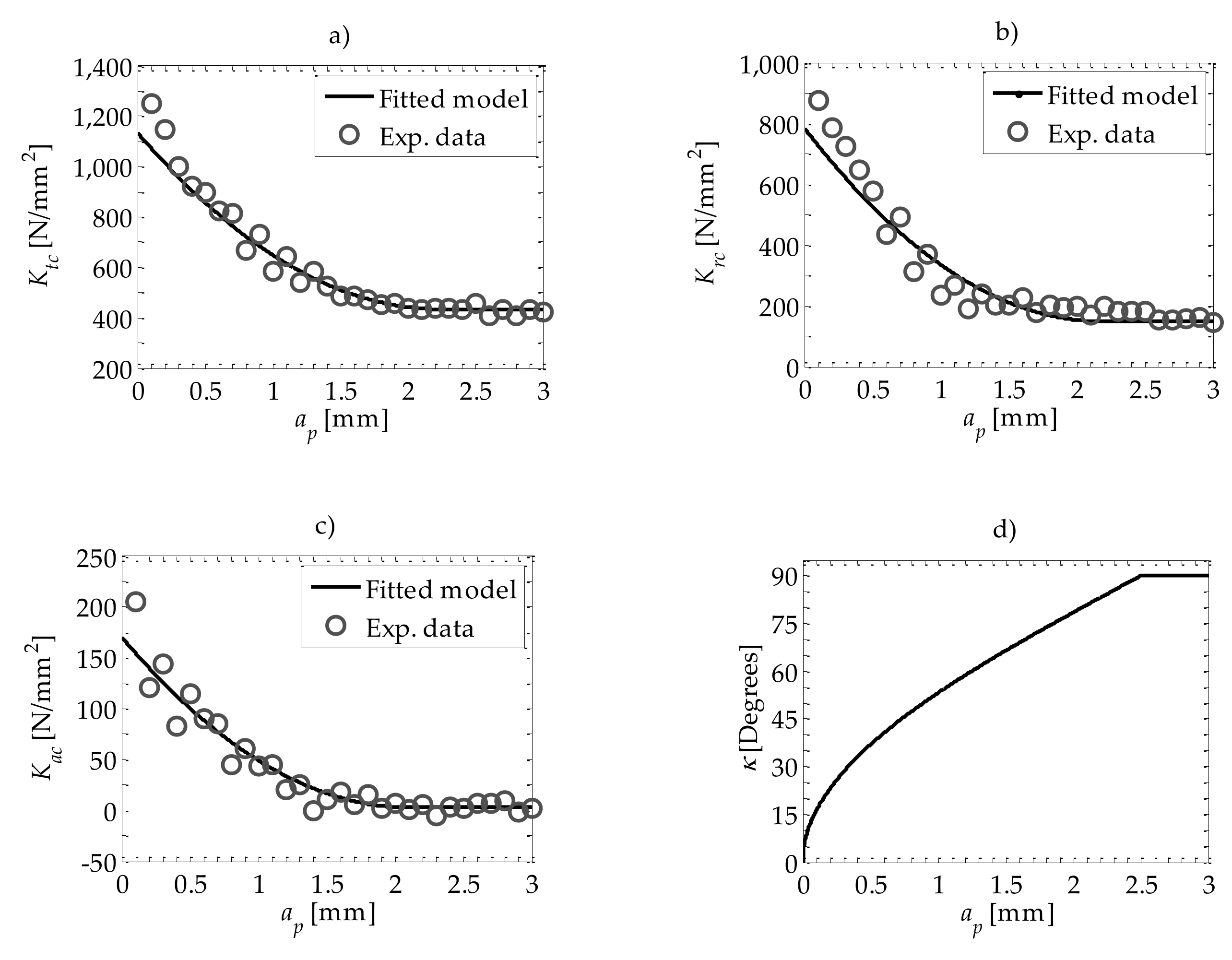
2.2. Characterization Procedure

The characterization procedure assumes the linear relationship between the averaged cutting forces $\tilde{F}$ and the feed rate f_z. This relationship is established as follows:

$$\tilde{F}=f_z·\widetilde{F_c}+\widetilde{F_e}.$$

(4)

Here, $\widetilde{F_c}$ and $\widetilde{F_e}$ are the cutting shear and edge components, respectively. Developing Equation (4) in terms of differential cutting forces, the following expression is obtained:

$$F\left(\varphi \right)={{\displaystyle \int }}_{z_1}^{z_2}dF\left(\varphi ,z\right)={{\displaystyle \int }}_{z_1}^{z_2}d{F}_c\left(\varphi ,z\right)·f_z+{{\displaystyle \int }}_{z_1}^{z_2}d{F}_e\left(\varphi ,z\right).$$

(5)

To determine the average cutting force per tooth, Equation (5) is integrated within the limits of the entrance (${\varphi }_s$) and exit (${\varphi }_e$) angles, and it is divided by the pitch angle $2\pi /N_z$:

$$\tilde{F}=\frac{N_z}{2\pi }{{\displaystyle \int }}_{{\varphi }_s}^{{\varphi }_e}Fd\varphi .$$

(6)

Therefore, the Cartesian components of the average forces for the tool are:

$$\begin{gathered} {\tilde{F}}_{xc}=\frac{N_t}{2\pi }{{\displaystyle \int }}_{{\varphi }_s}^{{\varphi }_e}{{\displaystyle \int }}_{z_1}^{z_2}\left(K_{tc}\sin \varphi \cos \varphi \sin \kappa +K_{rc}{\sin }^2\varphi {\sin }^2\kappa -K_{ac}{\sin }^2\varphi \sin \kappa \cos \kappa \right)dzd\varphi \\ {\tilde{F}}_{yc}=\frac{N_t}{2\pi }{{\displaystyle \int }}_{{\varphi }_s}^{{\varphi }_e}{{\displaystyle \int }}_{z_1}^{z_2}\left(K_{tc}{\sin }^2\varphi \sin \kappa -K_{rc}\sin \varphi \cos \varphi {\sin }^2\kappa +K_{ac}\sin \varphi \cos \varphi \sin \kappa \cos \kappa \right)dzd\varphi \\ {\tilde{F}}_{zc}=\frac{N_t}{2\pi }{{\displaystyle \int }}_{{\varphi }_s}^{{\varphi }_e}{{\displaystyle \int }}_{z_1}^{z_2}\left(-K_{rc}\sin \varphi \sin \kappa \cos \kappa -K_{ac}{\sin }^2\varphi \sin \kappa \right)dzd\varphi . \end{gathered}$$

(7)

The final step consists of computing shear and edge coefficients by solving the system of Equation (7).

2.3. Experimental Procedure

A total of 120 cuttings were performed for 100% radial immersion in aluminum 7075T6 during dry machining. The forces were recorded by using a dynamometer 9257B (Kistler Group, Winterthur, Switzerland) for the set of cutting conditions listed in

Table 1. Characterization test parameters.

Spindle speed	3000 rpm
Radial Immersion	16 mm, down milling
Depth of cut $\left(a_p\right)$	0.1–3.0 [mm]
Feed per tooth (fz)	0.05, 0.10, 0.15, 0.20 [mm/tooth]

. The spindle speed is set at 3000 rpm based on the dynamometer’s natural frequency to avoid the amplification of milling forces. The force signals were acquired using a VibSoft-20 acquisition card (Polytec GmbH, Waldbronn, Germany) at a sample rate of 48 kHz and processed in a custom-made MATLAB app to remove drift and noise phenomena.

Cutting forces data were collected for increments of 0.1 mm in the axial depth of cut with the aim of minimizing the model errors and obtaining detailed information of the cutting coefficients along the cutting edge in the toroid section. For a given axial depth of cut, four values of feed per tooth were tested as listed in Table 1.

For a set of experiments with a specific axial depth of cut, the system of Equations (7) is solved to obtain the $K_c$ and $K_e$ cutting coefficients. The computed data were fitted by using a second-order polynomial function as listed in

Table 2. Cutting coefficients of the tool.

Cutting Coefficients	Toroid [N/mm2]	Flank [N/mm2]
$K_{tc}$	$138.89z^2$−$625z+1136.9$	434
$K_{rc}$	$132.98z^2-581.96z+785.4$	149.3
$K_{ac}$	$37.57z^2-159.06z+171.06$	2.8

.

Figure 3 displays the fitted model for shear coefficients in the tool coordinate system (tangential, radial, and axial directions). It can be seen from Figure 3 that the cutting coefficients, in the range of 0.1–1.5 mm, change significantly whereas for the section approaching the flank section of the cutting edge, these remain almost constant. This can be explained from Figure 3d, in which the cutting-edge angle starts from zero at the bottom of the cutting edge and increases to 90° at the flank tool section. In a square end mill, where the cutting-edge angle is 90° at any edge location, the cutting coefficients remain constant. However, for the bull-nose end mill, the cutting coefficient exhibits nonlinear behavior. For this reason, the proposed mechanistic model is important to predict accurately stability boundaries.

Notice from Figure 3a–c that the cutting coefficients in all directions present high values for the toroid section: almost three times higher in the radial direction (see Figure 3b), and almost five times higher in the axial direction (see Figure 3c) compared to the flank section of the cutting edge, which could affect significantly the critical depth of cut of thin-floors machining.

In order to validate the proposed model, slot milling tests were performed. Figure 4 shows the comparison between the proposed cutting force-fitted model and experimental forces for two sets of cutting conditions. The accuracy of the proposed model to fit experimental data is shown in Figure 4; it is evident that in both cases, the proposed forced model predicts the experimental data well.

3. Stability Analysis and Experimental Validation

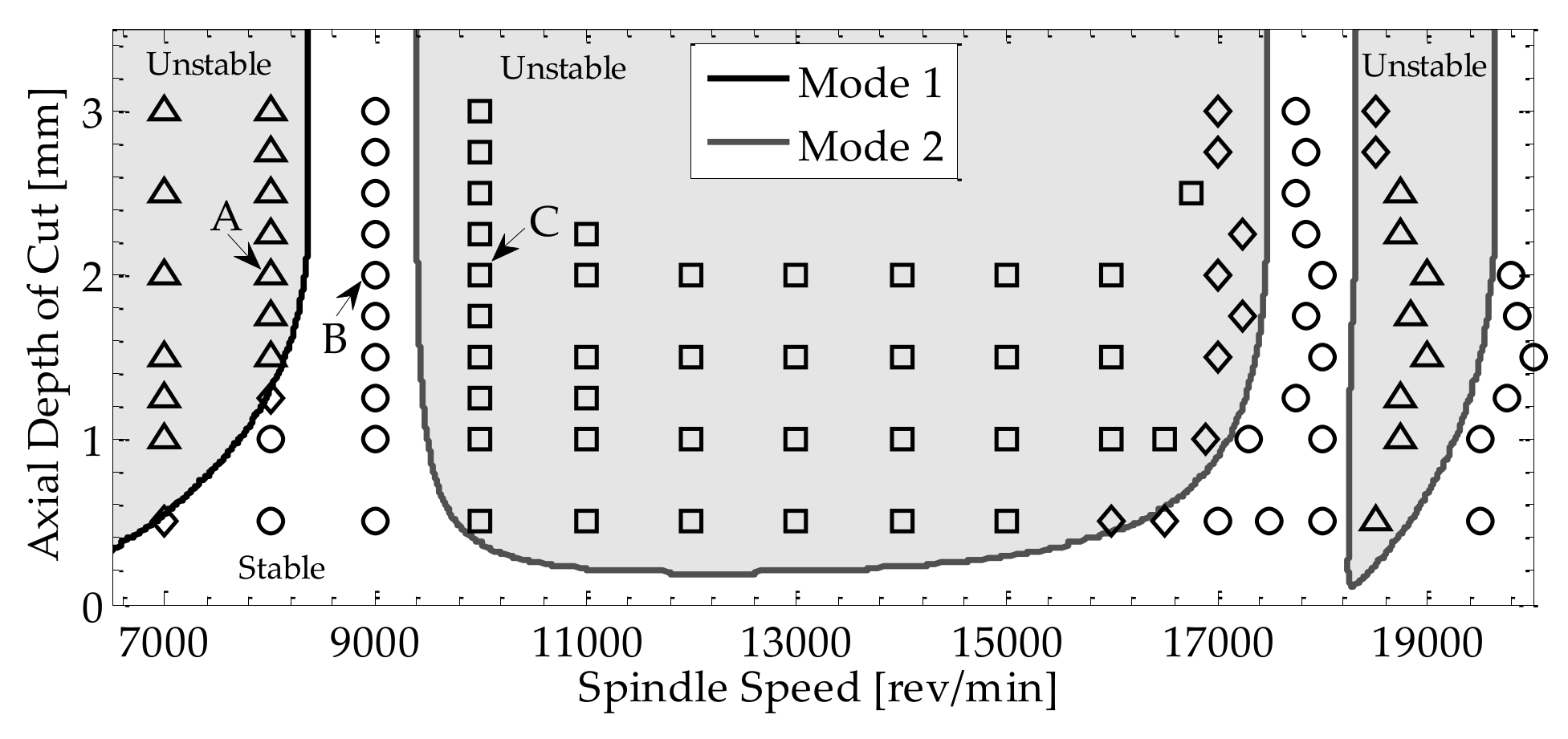
3.1. Stability Analysis for Thin-Floor Machining

In finish milling operations of thin-floor components where the dominant mode is oriented in the z-direction, the stability model can be simplified considering only the Frequency Response Function (FRF) of the thin floor, so the system becomes a one degree of freedom (1 dof) model as described by Campa et al. [30]. In this case, the dynamic chip thickness is determined from:

$$h\left({\varphi }_j\left(t\right)\right)=\cos \kappa \Delta z$$

(8)

where ${\varphi }_j\left(t\right)$ is the angular position of the cutting edge $j$ and $\Delta z=\left(z\left(t\right)-z\left(t-\tau \right)\right).$ The equation of motion that describes the dynamics of the thin floor is given as:

$$\ddot{z}\left(t\right)+2\zeta {\omega }_n\dot{z}\left(t\right)+{\omega }_n^{2}z\left(t\right)=\frac{F_z\left(t\right)}{m_m}\left(z\left(t\right)-z\left(t-\tau \right)\right)$$

(9)

where $m_m$ is the modal mass, $\zeta$ describes the damping ratio, ${\omega }_n$ is the angular natural frequency, and $F_z$ is the cutting force in the z-direction, which is given as:

$$F_z\left(t\right)={{\displaystyle \sum }}_{j=0}^{N_t-1}g\left({\varphi }_j\left(t\right)\right)h\left({\varphi }_j\left(t\right)\right)\left(-K_{rc}{\cos }^2\kappa -K_{ac}\sin \kappa \cos \kappa \right).$$

(10)

Here, $g\left({\varphi }_j\left(t\right)\right)$ is a switching function that returns the value of one when the tooth cutter is cutting and the value of zero otherwise. The matrix representation of Equation (9) becomes:

$$\dot{z}\left(t\right)=A\left(t\right)z\left(t\right)+B\left(t\right)z\left(t-\tau \right)$$

(11)

where $z={\left[z,\dot{z}\right]}^T$, $A\left(t+\tau \right)=A\left(t\right)$, $B\left(t+\tau \right)=B\left(t\right)$, and $\tau$ is the time delay. Following the Enhanced Multistage Homotopy Perturbation Method (EMHPM) described in [34], Equation (11) is written in an equivalent form as:

$${\dot{z}}_i\left(T\right)-A_t{z}_i\left(T\right)\approx B_t{z}_i^{\tau }\left(T\right)$$

(12)

where $z_i\left(T\right)$ indicates the m-order solution for Equation (11) that satisfies the initial conditions $z_i\left(0\right)=z_{i-1}$, $A_t$ and $B_t$ are the periodic matrix whose values vary with time $t$. The period $\left[t_0-\tau ,t_0\right]$ is discretized in N points to approximate the term $z_i^{\tau }\left(T\right)$ to the delay in Equation (12). The function $z_i^{\tau }\left(T\right)$ could be approximate as a first-polynomial representation:

$$z_i^{\tau }\left(T\right)\approx z_{i-N}+\frac{N-1}{\tau }\left(z_{i-N+1}+z_{i-N}\right)T$$

(13)

Next, we define $z_i\equiv z_i\left(T_i\right)$ and then, Equation (12) is substituted into Equation (13) to get:

$${\dot{z}}_i=A_t{z}_i+B_t{z}_{i-N}-\frac{N-1}{\tau }{B}_t{z}_{i-N}T+\frac{N-1}{\tau }{B}_t{z}_{i-N+1}T$$

(14)

where

$$A_t=\left[\begin{array}{cc}0& 1\\ -{\omega }_n{}^2+\frac{F_z\left(t\right)}{m_m}& -2\zeta {\omega }_n\end{array}\right],B_t=\left[\begin{array}{cc}0& 0\\ -\frac{F_z\left(t\right)}{m_m}& 0\end{array}\right].$$

(15)

To compute the stability lobes of Equation (14), the procedure described in [26] is followed. Then, it is assumed that Equation (14) can be written as a function of discretized states:

$$z_i\left(T\right)\approx P_i\left(T\right)z_{i-1}+Q_i\left(T\right)z_{i-N}+R_i\left(T\right)z_{i-N+1}$$

(16)

where

$$\begin{gathered} P_i\left(T\right)={\displaystyle \sum }_{k=0}^m\frac{1}{k!}{A}_t^k{T}^k, \\ Q_i\left(T\right)=\left\{\begin{array}{c}{\displaystyle {\displaystyle \sum }_{k=1}^m}\frac{N-1}{\left(k+1\right)!\left(\tau \right)}{A}_t^{k-1}{B}_t{T}^{k+1} m\ge 1\\ 0 m=0 \end{array}\right. \\ {R}_i\left(T\right)=\left\{\begin{array}{c}{\displaystyle \sum }_{k=1}^m\frac{1}{k!}{A}_t^{k-1}{B}_t{T}^k-Q_m m\ge 1\\ 0 m=0\end{array}\right.. \end{gathered}$$

(17)

Thus, the approximate solution of Equation (16) can be written as a discrete map $w_i=D_i{w}_{i-1}$. By following the Floquet theory [35,36], the transition matrix $\Phi$ of Equation (16) is calculated over period $\tau =\left(N-1\right)\Delta t$ by coupling each solution of $D_i, i=1,2,\dots N-1$ to get:

$$\Phi =D_{N-1}{D}_{N-2}\dots D_2{D}_1.$$

(18)

Finally, the stability lobes of Equation (11) are determined by computing the eigenvalues of the transition matrix. Notice that the 1 dof model proposed in Equation (9) assumes a single vibration mode; however, its application to a multi-degree of freedom system could be performed by computing the stability lobes for each mode.

3.2. Experimental Validation of Stability Lobes

Experimental milling cutting tests were performed in a Makino F3 machining center. A monolithic cantilever beam of 116 × 177 × 12.7 mm was used to mimic a 1 dof thin-floor behavior in the z-direction defined as shown in Figure 5. A 7075T6 aluminum workpiece was positioned on the cantilevered plate using two screws to maintain its dynamic characteristics during several passes (total mass does not change substantially). In the thin-floor milling process, the cutting tool is much stiffer in comparison with the workpiece properties. For that reason, the dynamic response of a thin floor is the most important factor during machining. The workpiece FRF was measured with a compact laser vibrometer, model CLV-2534 (Polytec GmbH, Waldbronn, Germany) and a impulse force hammer, Model 9722A (Kistler Group, Winterthur, Switzerland). The fitted modal parameters listed in

Table 3. Measured modal parameters of the workpiece.

$\mathbf{Mode}\mathit{z}$	f [Hz]	k [N/m]	$\mathit{\xi }$
1	93	6.59E5	0.003
2	304	4.89E6	0.004

were performed using CutPro Simulation Software (Manufacturing Automation Laboratories Inc., Vancouver, BC, Canada).

In order to validate the dynamics of the milling process together with the proposed cutting force model, stability lobes for 2.5 mm radial immersion were computed and shown in Figure 6 by using the EMHPM of Equation (11). As described in Section 2.2, the cutting forces model was considered for a range from 0 to 3 mm in the z-direction. The stability lobes verification was studied through the measurement of the vibrations of the workpiece mounted on the cantilevered plate. An accelerometer type 8778A500M14 (Kistler Group, Winterthur, Switzerland). weighing 0.4 g was used to acquire the vibrations, and a tachometer model FS-V31 (Keyence Corporation, Osaka, Japan) was used to detect every single revolution of the spindle as shown in Figure 5.

The signal processing consisted of two steps. First, raw signals were filtered with a low-pass filter with a cut-off frequency of 5 kHz. Additionally, the tachometer signal was manipulated to include a virtual pulse in the middle of two consecutive detected pulses that allows us to sample the accelerometer signal according to the tool passing period (two flutes impact the workpiece during each revolution). Secondly, the analysis of the accelerometer signal was performed via wavelet transform (CWT), power spectral density (PSD), and Poincaré diagrams. By comparing experimental and theoretical chatter frequencies [37], all this information was used to identify and categorize every single cutting test as having stable or unstable cutting parameters. After completing the signal process and categorization, experimental data were superposed in Figure 6.

The stable cuts in Figure 6 are denoted by circles, the unstable quasi-periodic cuts are denoted by squares, and the unstable double periodic cuts are denoted by triangle symbols. Experimental results denoted by diamonds represent experimental conditions without dominant chatter frequencies, which makes the classification as either unstable or stable challenging.

From Figure 6, three cutting tests that describe typical stable/unstable behavior have been selected (points A, B, and C). Point A describes unstable period-doubling chatter, Point B describes stable cutting conditions, and Point C describes unstable double periodic. Since the CWT analysis allows us to observe how frequencies evolve in the time domain, then this analysis was applied to accelerometer data as shown in Figure 7a–c. To relate the detected frequency in relation to the excitation, the following normalized frequency is introduced:

$$f_n=f_w/f_{TPE}.$$

(19)

In Equation (19), $f_w$ represents the wavelet transform frequency and $f_{TPE}$ represents the tooth passing excitation frequency. The overlapped circles and cross white marks in Figure 7a–c identify normalized frequencies of $f_n=1$ and $f_n=0.5$ , respectively. In Figure 7d,e, the acceleration sampling (red circles) denotes vibration amplitude when the cutting tool hits the workpiece. Poincare diagrams (Figure 7g–i) were constructed with the acceleration sampling data versus 20-delayed samples. The power spectral density (PSD) in Figure 7j–l describes the power density from the acceleration data in the frequency domain.

Point A (Figure 7a,d,g,j) exhibits unstable period-doubling chatter, meaning that each tooth passing the excitation period is half of the dominant period in the acceleration signal. Even the PSD plot (Figure 7j) exhibits several chatter frequencies, while the doming frequency almost coincides with the cross marks, which confirms the period-doubling chatter. Due to all these chatter frequencies, the Poincaré diagram in Figure 7g draws two semi-elliptical trajectories. This behavior contrasts with a pure period-double chatter experiment (data not shown) that draws two concentration of samples; in other words, the workpiece vibrates with a dominant frequency that is half that of the tool passing excitation frequency.

Point B (Figure 7b,e,h,k) shows stable cutting conditions. In this case, the dominant frequency in the CWT is related to the tool passing frequency (circle marks) during several revolutions. Notice as well that for each period τ, two stains appear corresponding to one vibration cycle: one peak and one valley. As a result, the peak frequencies in the PSD plot coincide with multiples of the tool passing frequency. A Poincaré diagram for stable cutting (Figure 7h) shows the concentration of sampled acceleration data, meaning the vibration amplitude is similar every time a flute hits the workpiece.

Point C describes Hopf instabilities; this instability draws in the PSD plot-dominant quasi-periodic chatter frequencies. Notice that the frequency intensity in the CWT (Figure 7c) is below normalized frequency f_n = 1, and those values change in time. In contrast with Point A and B, the PSD (Figure 7l) shows multiple chatter frequencies, which are responsible for several loops in the Poincaré diagram.

4. Semi-Active Magnetorheological Damper Device for Chatter Mitigation

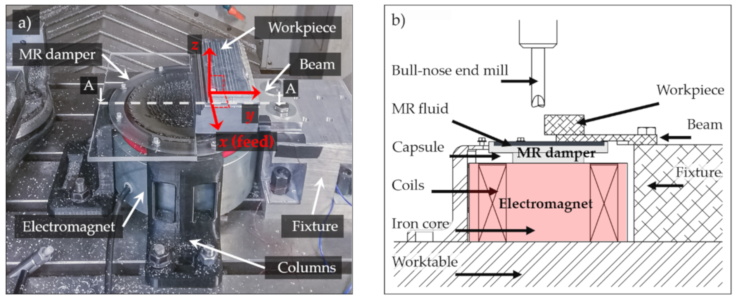
4.1. Experimental Setup of MR Damper Assembly

The experimental setup is implemented as shown in the optical photograph (Figure 8a). This system uses the same components described in Section 3.2, but now, it also includes the semi-active MR damper device. The MR damper device is a pool-like container or chamber fabricated in acrylic material; a non-magnetic material avoids reducing the magnetic flux density generated by an electromagnet. The acrylic chamber contains the magnetorheological fluid with an internal diameter of 200 mm and 19 mm height. In order to avoid spills, an acrylic plate is placed covering the area not in contact with the beam. The MR damper assembly is supported with 3D-printed columns so that an electromagnet could be placed between the worktable and the MR damper. An HP/Agilent power supply, model 6032A was connected to a electromagnet, model VEM200 (Electroimanes NAFSA, Gernika, Spain), which accepts a maximum input current of 3.4 A at 25 V. Once the electromagnet is energized independently of the machining, it generates a magnetic flux density that changes the yield stress of the MR fluid. The chamber was fully filled with an MRF-122EG MR fluid (LORD Corporation, Cary, NC, USA).

The cross-section A – A presented in Figure 8b shows a better view of the experimental setup and allows us to observe that the beam is sunk about 1 mm in the MR fluid with a contact area of about 50 cm². It is important to sink the beam to guarantee that it is always in contact with the MR fluid during machining, because the amplitude of the vibrations is expected to be in the range of ± 1 mm. Once the workpiece is attached to the beam, the experimental setup is ready for FRF measurements and experimental milling cuttings.

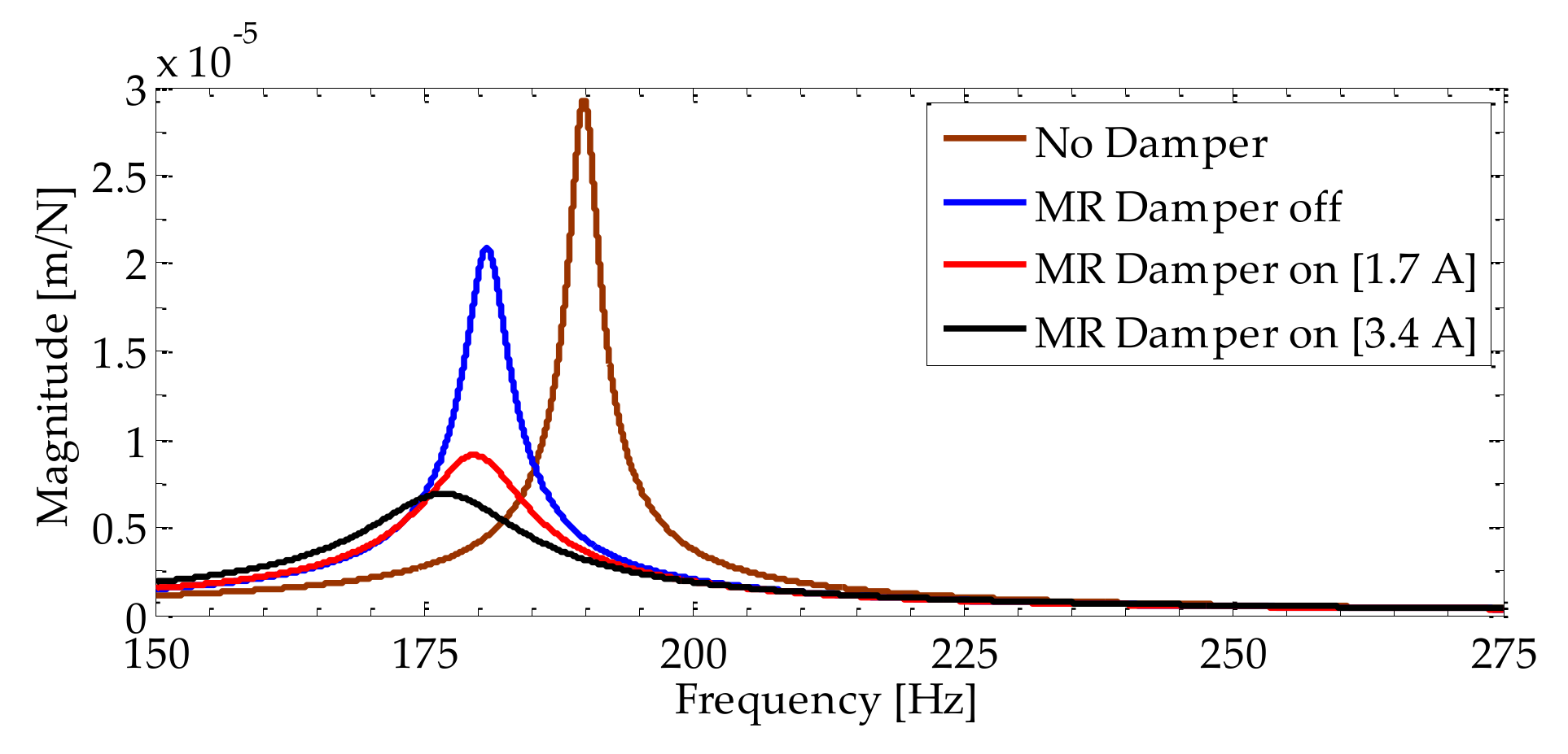
4.2. Modified FRF of the Cantilever Beam

For this experimental setup, to validate the effectiveness of the MR damper device, a new cantilever beam made of aluminum alloy 7075T6 was designated with dimensions of 103 × 127 × 12.7 mm to induce specific modal parameters and study the stability boundaries of thin walls with a very low critical depth value (below 0.5 mm). In order to evaluate the effects of the MR damper over the stability boundaries, three levels of MR damper performance were studied: highest, 3.4 A; medium, 1.7 A; and lowest, off. The magnetic flux density produced by the electromagnet was measured experimentally with an F.W. BELL gaussmeter, model 5170. Figure 9 shows the magnetic flux density measured from the center of the cylindrical electromagnetic outwards along the radial direction. As expected, the magnitude of the magnetic flux density is almost constant in the radial direction, and the magnitude is proportional to the supplied electrical current. Measurements after 40 mm were not considered, since the cantilever beam was not in contact with the MR fluid.

The yield stress of the MR fluid changes depending on the magnetic flux density at which it is subjected. It is expected that the dynamic properties of the system imposed will be modified because of the effects of the MR damper device. The FRF was experimentally measured for 4 scenarios and plotted in Figure 10. The scenarios are (1) no damper, (2) damper off, (3) damper on with 1.7 A, and (4) damper on with 3.4 A. The technique used to acquire the FRF and the parameter fitting procedure are similar to those of Section 3.1.

Table 4. Modal parameters of the cantilever beam under the action of a semi-active MR damper device.

Electrical Current [A]	Average Magnetic Flux Density [G]	Yield Stress [KPa]	Natural Frequency f [Hz]	Stiffness k [N/m]	$\mathbf{Damping}\mathit{\xi }$
No Damper	-	-	190	2.40 × 106	0.007
Off–0	-	0	180	2.18 × 106	0.011
On–1.7	372	6	178	2.04 × 106	0.023
On–3.4	695	12	175	2.07 × 106	0.036

summarizes the modal parameters computed for each scenario.

Notice from Table 4 that the natural frequency of the beam, without a damper, is 190 Hz and the damping ratio is 0.007. When MR fluid is in contact with the thin floor and off, the natural frequency shifts to 180 Hz, and the damping ratio increased by about 50%. Note that when the MR damper is off, the electromagnet is not active, and no electrical current is provided, but it is still in contact with the cantilever beam and the FRF is affected. Table 4 shows that if the MR damper is turned on and subjected to two electrical currents values, the damping ratio of the system increases proportionally. The damping of the system depends on the yield stress of the magnetorheological fluid, which can be estimated by using the technical data sheet from the fluid manufacturer [38].

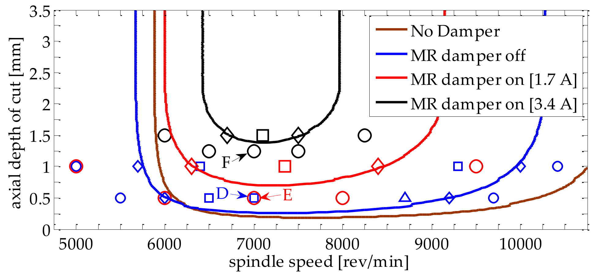
4.3. Experimental Determination of Stability Lobes under the Action of the MR Damper Device

Notice when the MR damper device was placed on the cantilever beam, the damping ratio of the beam change substantially, as listed in Table 4. Once the modal parameters were computed, the stability lobes were plotted in Figure 11 following the same methodology described in Section 3.1. Since the MR damper device increases the damping ratio in the system, the stability boundaries not only shift toward higher axial depth but also shrink, which substantially allows more productive cutting combinations. For instance, when the MR damper device is turned off and cuts are performed at 7000 rev/min, the critical axial depth of cut is close to 0.25 mm, but this value increases to 0.75 and to 1.4 mm when the current in the MR damper is adjusted at 1.7 and to 3.4 A, respectively. In order to validate the effect of the MR damper over the stability behavior, three cutting tests were selected, and these were named points D, E, F as illustrated in Figure 11. All of them correspond to spindle speeds of 7000 rpm but with different axial depth-of-cut values and subjected to specific scenarios. The accelerometer signal of point D was acquired when the MR damper was turned off, while the acceleration for points E and F were collected when the MR damper was turned on with 1.7 and 3.4 A, respectively.

Figure 12a shows the CWT obtained from the acceleration signal collected for point D (a_p = 0.5 mm). Notice that this CWT plot illustrates dominant frequencies (red colors) lower than the normalized f_n = 1, which indicates that cutting is an unstable quasi-periodic chatter test, as predicted by the stability lobes in Figure 11. This is also confirmed with the sampled acceleration signal plotted in Figure 12d, since the amplitudes of the samples are not similar. The same combination of cutting parameters (a_p = 0.5 mm and n = 7000 rev/min) are now analyzed when the MR damper device is turned on with 1.7 A. Notice from Figure 12b that for this cutting test (point E), the CWT describes dominant frequencies that are very close to normalized frequency f_n = 1, and thus, this is an indication of stable cutting conditions. This result agrees with the stability lobes plotted in Figure 11, since the location of point E indicates stable cutting conditions because it is below the critical axial depth of cut value of 0.75 mm. Similarly, point F (a_p = 1.25 mm) exhibits stable cutting conditions, since the critical depth of cut has now the value of 1.5 mm. It is important to observe that the acceleration amplitude for experimental test F (Figure 12f) is even lower than the value recorded for point E (Figure 12e), confirming that the MR damper device offers higher damping and is an effective technique to avoid unstable vibrations.

5. Conclusions

Chatter vibration during the milling process of thin-floor components is a key factor that limits productivity. Placing an MR fluid in contact with the thin floor modifies the damping ratio without changing the natural frequency and modal stiffness. Experimental measurements indicate that a good degree of accuracy is attained from the proposed cutting force model, which is a key factor to predict stability lobes during the machining of thin floors using a bull-nose end mill.

• The proposed force model in which the tool edge is discretized in disks along the z-direction predicts the experimental cutting forces with high accuracy.
• The predicted EMHPM stability lobes of the cantilever beam closely follow experimental data.
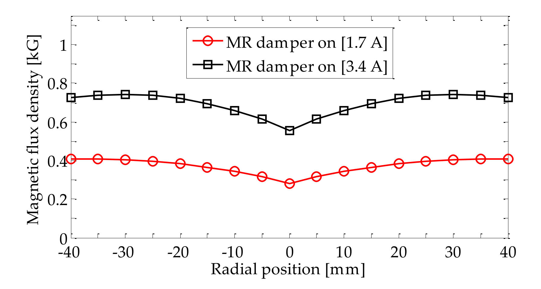
• The use of an MR damper device located under the cantilever beam modifies modal damping depending on the magnitude of the magnetic flux density. For the higher magnetic flux density values, the damping ratio increases about 4 times, while the modal stiffness slightly varies.
• Under the effect of the MR damper device, the stability boundaries shift toward higher critical axial depth of cut values, which substantially enhances stable cutting conditions. In other words, experimental measurements indicate that when using the MR damper device, it is possible to increase the critical depth of cut from 0.5 to 1.5 mm in the range of spindle speed from 7000 to 10,000 rev/min, with an increase in the material removal rate and productivity by a factor of at least 3.
• The use of a semi-active MR damper device represents an alternative way to increase productivity while machining thin-floor components because of its robustness and adaptability to complex geometries. Since MR fluids can modify their yield and shear stresses as a function of the applied magnetic flux density, the damping ratio can be adjusted as needed in order to reach stable cutting conditions. Additionally, the semi-MR damper device is simple to operate versus its counterpart, the active MR damper device, which needs sensors and real-time data processing.

References

1. Del Sol, I.; Rivero, A.; De Lacalle, L.N.L.; Gamez, A.; De Lacalle, L.N.L. Thin-Wall Machining of Light Alloys: A Review of Models and Industrial Approaches. Materials 2019, 12, 2012. [Google Scholar] [CrossRef] [PubMed] [Green Version]
2. Ahmed, G.S.; Reddy, P.R.; Seetharamaiah, N. Experimental Evaluation of Metal Cutting Coefficients under the Influence of Magneto-rheological Damping in End Milling Process. Procedia Eng. 2013, 64, 435–445. [Google Scholar] [CrossRef] [Green Version]
3. Junbai, L.; Kai, Z. Multi-point location theory, method, and application for flexible tooling system in aircraft manufacturing. Int. J. Adv. Manuf. Technol. 2010, 54, 729–736. [Google Scholar] [CrossRef]
4. Kalocsay, R.; Kolvenbach, C. Innoclamp GmbH–Hydraulic Clamping Systems. Available online: https://www.innoclamp.de/. (accessed on 28 June 2020).
5. Woody, S.C.; Smith, S.T. Damping of a thin-walled honeycomb structure using energy absorbing foam. J. Sound Vib. 2006, 291, 491–502. [Google Scholar] [CrossRef]
6. Park, G.; Bement, M.; Hartman, D.A.; Smith, R.E.; Farrar, C.R. The use of active materials for machining processes: A review. Int. J. Mach. Tools Manuf. 2007, 47, 2189–2206. [Google Scholar] [CrossRef]
7. Zhu, X.; Jing, X.; Cheng, L. Magnetorheological fluid dampers: A review on structure design and analysis. J. Intell. Mater. Syst. Struct. 2012, 23, 839–873. [Google Scholar] [CrossRef]
8. Symans, M.D.; Constantinou, M.C. Semi-active control systems for seismic protection of structures: A state-of-the-art review. Eng. Struct. 1999, 21, 469–487. [Google Scholar] [CrossRef]
9. Ji, H.; Huang, Y.; Nie, S.; Yin, F.; Dai, Z. Research on Semi-Active Vibration Control of Pipeline Based on Magneto-Rheological Damper. Appl. Sci. 2020, 10, 2541. [Google Scholar] [CrossRef] [Green Version]
10. Díaz-Tena, E.; Marcaide, L.L.D.L.; Gómez, F.C.; Bocanegra, D.C. Use of Magnetorheological Fluids for Vibration Reduction on the Milling of Thin Floor Parts. Procedia Eng. 2013, 63, 835–842. [Google Scholar] [CrossRef] [Green Version]
11. Fleischer, J.; Denkena, B.; Winfough, B.; Mori, M. Workpiece and Tool Handling in Metal Cutting Machines. CIRP Ann. 2006, 55, 817–839. [Google Scholar] [CrossRef]
12. Segalman, D.; Redmond, J. Chatter suppression through variable impedance and smart fluids. SMART Struct. Mater. 1996, 53, 1689–1699. [Google Scholar]
13. Wang, M.; Fei, R. Chatter suppression based on nonlinear vibration characteristic of electrorheological fluids. Int. J. Mach. Tools Manuf. 1999, 39, 1925–1934. [Google Scholar] [CrossRef]
14. Mei, D.; Kong, T.; Shih, A.J.; Chen, Z. Magnetorheological fluid-controlled boring bar for chatter suppression. J. Mater. Process. Technol. 2009, 209, 1861–1870. [Google Scholar] [CrossRef]
15. Çeşmeci, Ş.; Engin, T. Modeling and testing of a field-controllable magnetorheological fluid damper. Int. J. Mech. Sci. 2010, 52, 1036–1046. [Google Scholar] [CrossRef]
16. Som, A.; Kim, N.-H.; Son, H. Semiactive Magnetorheological Damper for High Aspect Ratio Boring Process. IEEE/ASME Trans. Mechatron. 2015, 20, 1–8. [Google Scholar] [CrossRef]
17. Kishore, R.; Choudhury, S.K.; Orra, K. On-line control of machine tool vibration in turning operation using electro-magneto rheological damper. J. Manuf. Process. 2018, 31, 187–198. [Google Scholar] [CrossRef]
18. Zhang, Y.; Wereley, N.M.; Hu, W.; Hong, M.; Zhang, W. Magnetic Circuit Analyses and Turning Chatter Suppression Based on a Squeeze-Mode Magnetorheological Damping Turning Tool. Shock Vib. 2015, 2015, 1–7. [Google Scholar] [CrossRef] [Green Version]
19. Ma, J.; Zhang, D.; Wu, B.; Luo, M.; Liu, Y. Stability improvement and vibration suppression of the thin-walled workpiece in milling process via magnetorheological fluid flexible fixture. Int. J. Adv. Manuf. Technol. 2016, 88, 1231–1242. [Google Scholar] [CrossRef]
20. Olvera, D.; Urbicain, G.; Elías-Zúñiga, A.; De Lacalle, L.N.L.; De Lacalle, L.N.L. Improving Stability Prediction in Peripheral Milling of Al7075T6. Appl. Sci. 2018, 8, 1316. [Google Scholar] [CrossRef] [Green Version]
21. Campa, F.J.; De Lacalle, L.L.; Celaya, A.; De Lacalle, L.N.L. Chatter avoidance in the milling of thin floors with bull-nose end mills: Model and stability diagrams. Int. J. Mach. Tools Manuf. 2011, 51, 43–53. [Google Scholar] [CrossRef] [Green Version]
22. Budak, E.; Altintaş, Y.; Armarego, E.J.A. Prediction of Milling Force Coefficients From Orthogonal Cutting Data. J. Manuf. Sci. Eng. 1996, 118, 216–224. [Google Scholar] [CrossRef]
23. Lee, P.; Altintaş, Y. Prediction of ball-end milling forces from orthogonal cutting data. Int. J. Mach. Tools Manuf. 1996, 36, 1059–1072. [Google Scholar] [CrossRef]
24. Yücesan, G.; Altintas, Y. Prediction of Ball End Milling Forces. J. Eng. Ind. 1996, 118, 95–103. [Google Scholar] [CrossRef]
25. Altintas, Y. Analytical Prediction of Three Dimensional Chatter Stability in Milling. JSME Int. J. Ser. C 2001, 44, 717–723. [Google Scholar] [CrossRef] [Green Version]
26. Olvera, D.; Elías-Zúñiga, A.; Martínez-Alfaro, H.; De Lacalle, L.L.; Rodríguez, C.A.; Campa, F.J.; De Lacalle, L.N.L. Determination of the stability lobes in milling operations based on homotopy and simulated annealing techniques. Mechatronics 2014, 24, 177–185. [Google Scholar] [CrossRef]
27. Urbikain, G.; Olvera, D.; De Lacalle, L.N.L.; Urbicain, G. Stability contour maps with barrel cutters considering the tool orientation. Int. J. Adv. Manuf. Technol. 2016, 89, 2491–2501. [Google Scholar] [CrossRef]
28. Smith, K.; Dvorak, D. Tool path strategies for high speed milling aluminum workpieces with thin webs. Mechatronics 1998, 8, 291–300. [Google Scholar] [CrossRef]
29. Seguy, S.; Campa, F.J.; De Lacalle, L.N.L.; Arnaud, L.; Dessein, G.; Aramendi, G. Toolpath dependent stability lobes for the milling of thin-walled parts. Int. J. Mach. Mach. Mater. 2008, 4, 377. [Google Scholar] [CrossRef]
30. Campa, F.J.; De Lacalle, L.N.L.; Lamikiz, A.; Sanchez, J.A.; Lamikiz, A. Selection of cutting conditions for a stable milling of flexible parts with bull-nose end mills. J. Mater. Process. Technol. 2007, 191, 279–282. [Google Scholar] [CrossRef]
31. Altıntaş, Y.; Lee, P. Mechanics and Dynamics of Ball End Milling. J. Manuf. Sci. Eng. 1998, 120, 684–692. [Google Scholar] [CrossRef] [Green Version]
32. Altintas, Y. Manufacturing Automation. 2011. Appl. Mech. Rev. 2001, 54, B84. [Google Scholar]
33. Compeán, F.; Olvera, D.; Campa, F.J.; De Lacalle, L.L.; Elías-Zúñiga, A.; Rodríguez, C.A.; De Lacalle, L.N.L. Characterization and stability analysis of a multivariable milling tool by the enhanced multistage homotopy perturbation method. Int. J. Mach. Tools Manuf. 2012, 57, 27–33. [Google Scholar] [CrossRef]
34. Olvera-Trejo, D.; Zúñiga, A.; De Lacalle, L.N.L.; Rodríguez, C.A. Approximate Solutions of Delay Differential Equations with Constant and Variable Coefficients by the Enhanced Multistage Homotopy Perturbation Method. Abstr. Appl. Anal. 2015, 2015, 1–12. [Google Scholar] [CrossRef] [Green Version]
35. Insperger, T.; Stepan, G. Updated semi-discretization method for periodic delay-differential equations with discrete delay. Int. J. Numer. Methods Eng. 2004, 61, 117–141. [Google Scholar] [CrossRef]
36. Mei, Y.; Mo, R.; Sun, H.; He, B.; Bu, K. Stability Analysis of Milling Process with Multiple Delays. Appl. Sci. 2020, 10, 3646. [Google Scholar] [CrossRef]
37. Insperger, T.; Stepan, G.; Bayly, P.V.; Mann, B. Multiple chatter frequencies in milling processes. J. Sound Vib. 2003, 262, 333–345. [Google Scholar] [CrossRef]
38. Lord Corp, MRF-122EG Magneto-Rheological Fluid. Available online: http://www.lordmrstore.com/lord-mr-products/mrf-122eg-magneto-rheological-fluid. (accessed on 29 June 2020).
Figure 1. Composition of optical microscope photographs of the bull-nose end mill taken with an Alicona microscope: (a) bottom view (diameter measurement); (b) frontal view (nose radius measurement); (c) lateral view (helix angle measurement).
Applsci 10 05313 g001
Figure 2. Main cutting parameters in milling operation with a bull-nose end mill: axial discretization and differential cutting force components.
Applsci 10 05313 g002
Figure 3. Experimental cutting coefficients (circle marks) vs. fitted model (solid lines) along the toroidal section: (a) tangential; (b) radial; (c) axial directions; (d) κ angle along the toroid section.
Applsci 10 05313 g003
Figure 4. Comparison between experiment data and the proposed force model at 3000 rev/min and the cutting conditions: (a) ap = 0.5 mm, fz = 0.2 mm/tooth; (b) ap = 1.5 mm, fz = 0.15 mm/tooth.
Applsci 10 05313 g004
Figure 5. Experimental setup used for stability verification. An accelerometer is attached in the workpiece to detect vibrations, while the optical sensor is used to measure the spindle rotation.
Applsci 10 05313 g005
Figure 6. Predicted stability lobes obtained from Equation (11) together with experimental data in a down-milling operation. (○ stable cut, □ quasi-periodic chatter, Δ double periodic chatter, and ◊ border cutting parameters).
Applsci 10 05313 g006
Figure 7. Continuous wavelet transforms (a,b,c), sampled acceleration signals (d,e,f), Poincaré diagrams (g,h,i), and power spectral density (j,k,l) for unstable cut A (a,d,g,j), stable cut B (b,e,h,k), and quasi-periodic unstable cut C (c,f,i,l).
Applsci 10 05313 g007aApplsci 10 05313 g007b
Figure 8. (a) Optical image of the experimental setup and magnetorheological (MR) damper installation; (b) Schematic of cross-section A–A, the assembling of capsule–MR fluid is placed above the electromagnet.
Applsci 10 05313 g008
Figure 9. MR damper device magnetic flux density distribution.
Applsci 10 05313 g009
Figure 10. Measured Frequency Response Function (FRF) of the thin floor with the MR damper.
Applsci 10 05313 g010
Figure 11. Stability lobes diagrams for three scenarios of magnetic flux density applied to the MR damper device together with experimental data in a down-milling operation. (○ stable cut, □ quasi-periodic chatter, Δ double periodic chatter, and ◊ border cutting parameters).
Applsci 10 05313 g011
Figure 12. Analysis of the collected accelerometer signals (D, E and F) for different MR damper magnetic flux density values. Continuous wavelet transforms (a,b,c). Sampled acceleration signals (d,e,f).
Applsci 10 05313 g012