Abstract
The parabolic trough solar collector (PTC) is the most mature solar concentrating technology, and this technology is applied in numerous thermal applications. Usually, the thermal efficiency of the PTC is expressed with the aid of polynomial expressions. However, there is not a universal expression that is applied in all cases with high accuracy. Many studies use expressions with the first-degree polynomial, second-degree, or fourth-degree polynomial expressions. In this direction, this work is a study that investigates different expressions about the thermal efficiency of a PTC with a systematic approach. The LS-2 PTC module is examined with a developed numerical model in the Engineering Equation Solver for different operating temperatures and solar beam irradiation levels. This model is validated using experimental literature data. The found data are approximated with various polynomial expressions with up to six unknown parameters in every case. In every case, the mean absolute percentage error and the R2 are calculated. According to the final results, the use of the third power term leads to the best fitting results, as well as the use of the temperature difference term (ΔΤ), something that is new according to the existing literature. More specifically, the final suggested formula has the following format: “ηcol = a0 + a3∙ΔT3/Gb + b∙ΔΤ”. The results of this work can be used by the scientists for the optimum fitting of the PTC efficiency curves and for applying the best formulas in performance determination studies.
1. Introduction
The parabolic trough solar collector (PTC) is one of the most mature solar concentrating technologies [1] which can be used in numerous applications such as electricity production [2], industrial heat [3], refrigeration [4], space-heating [5], chemical processes [6] and polygeneration [7]. This collector is a linear concentrating technology that operates with a single-axis tracking system in the majority of the cases. There are only a few investigations with two-axis tracking systems but these designs are complex and they have a high cost. The most usual receiver is an evacuated tube absorber in order to operate in high temperatures with a satisfying efficiency [8]. The operation with thermal oil (e.g., Therminol VP-1) is able to reach up to 400 °C [9], while with the proper molten salts (e.g., nitrate salt), there is the possibility for operation up to 600 °C [10]. The use of gas working fluids (e.g., air or CO2) gives the possibility to operate in higher temperatures up to 1000 °C [11].
The literature includes numerous studies that incorporate PTC as the main or the secondary thermal energy source. Usually, the simulation of the PTC performance is conducted by using a thermal efficiency expression formula. The thermal efficiency of the solar collector is the ratio of the useful heat production to the available solar irradiation on the collector aperture (ηcol = Qu/Qs). Numerous formulas in the literature can be found and so it is interesting to present them as below.
A great percentage of the literature uses a simple linear expression for the determination of the efficiency. For example, the study of Kalogirou [12] approximates the PTC performance with a linear expression and it compares it with other linear formulas from the literature. This idea has also been used in newer studies such as in Coccia et al. [13]. Below, the linear expression is given:
The previous formula is usually used for the flat plate systems according to Duffie and Beckman [14]. Thus, this linear expression can be an accurate choice for PTC systems that operate to low-temperature levels up to 100 °C. Moreover, the previous formula is also known as the Hottel-Whillier-Bliss equation.
The next part of the literature studies uses a second-order expression which is in accordance with the ISO 9806-1 [15]. The goal of this formula is to better approximate the operating points of higher temperature levels.
This formula has been used by a great part of the recent literature studies. For example, Bellos et al. [16] selected an expression as the previous one for approximating the Eurotrough module performance. In another older work, Kalogirou and Panayiotou [17] conducted experimental work with PTC and they compared the approximation of the efficiency with a linear and a second-term formula. They concluded that both expressions are accurate and the second-order formula can be applied for the cases with higher temperatures.
An alternative expression of the previous one has been introduced by Dudley et al. [18] in an experimental work about LS-2. They tried to add an extra term with (Tin − Tam) without the incorporation of the solar beam irradiation:
Kutscher et al. [19] used a third-degree polynomial in order to approximate the PTC thermal efficiency and they found high values for the R2. More specifically, they tested the SkyTrough module with a Schott PTR-80 receiver.
They also tried to approximate the results with an alternative formula, as below:
A complex polynomial expression has been suggested by Nems and Kasperski [20] which incorporates the wind speed (Vw) as an extra parameter which includes a third-order term (Gb ∙ Tin ∙ Vw), as below:
The next part of the literature studies includes fourth-order terms. These formulas try to take into account the radiation thermal losses in a proper way because they are dependent on the fourth power of the absorber temperature level. Sallaberry et al. [21] tried to approximate the thermal losses with an expression with a fourth power and then the following expression for the thermal efficiency has been found:
They stated that this expression is in accordance with the standard IEC 62727 [22]. The use of the “cos (θ)” in the denominator is justified due to the approximation of the thermal losses for specific heat input. Practically, the thermal losses have to be normalized in every case in the absorbed irradiation, and the use of the cosine is a good choice for the approximation of the incident angle modifier. The thermal efficiency was calculated by reducing the thermal losses from the absorbed heat in every case.
Odeh et al. [23] have used a similar formula but they incorporated the wind speed inside the efficiency expression:
One alternative formula has been suggested also by Sallaberry et al. [24] which includes a fourth-order term and an order which takes into account the transient phenomena. The authors have expressed this formula in terms of “Qu/Aa”, but below, it is presented in terms of efficiency for having a uniform presentation style in the paper:
In another work, Sallaberry et al. [25] used a formula with an extra term, as below:
The previous formula is associated with the IEC 62862-3-2 standard which also suggests the use of a second-order term instead of the fourth-order term.
More specifically, the previous formula has been found by eliminating terms from the general formula according to DIS/ISO 9806 (2017) [26], which indicates approximately the following:
where the “EL” is the longwave irradiance with wavelength over 3 μm. Moreover, it has to be said that Sallaberry et al. [25] compared Equation (10) with Equation (12). They stated that formula (10) is slightly better than Formula (12) but the difference is negligible.
Xu et al. [27] used Formula (11) with all the terms in order to approximate the PTC performance. Furthermore, it has to be said that there are studies that tried to determine some analytical expressions for the PTC efficiency curves [28,29].
The previous literature review indicates that there is a huge interest in the literature in the approximation of the PTC thermal efficiency with effective expressions. Numerous formulas have been suggested and applied in literature studies. Moreover, there are some studies that compare different efficiency approximation equations. So, it is obvious that the researchers use various ways to approximate the PTC efficiency and there is not only one formula to expresses the thermal efficiency of a PTC. In this direction, this work comes to investigate different polynomial expressions that can be applied for the PTC thermal efficiency determination and they include the usual literature expressions. Moreover, these equations have extended in order to cover all the possible combinations of polynomial terms in a systematic way. Totally, 31 different equations are applied and evaluated according to two criteria: the mean absolute percentage error (MAPE) and the R2 index. To our knowledge, there is no other study in the literature like the present study, so this work adds something new to the existing literature. The results are discussed and the most important polynomial approximating formulas are presented. The final conclusions of this work indicate the most effective polynomial expressions for approximating the PTC efficiency by using the operating temperature levels and the solar irradiation, and also a clear comparison among the various polynomial formulas is given. Lastly, it is important to state that the operating points for the approximations are found by a developed model in the Engineering Equation Solver (EES) [30], which is validated with numerical experimental results.
2. Material and Methods
2.1. The Examined Collector
In this work, the module of the LS-2 PTC [18,31,32] is used in order to apply the different performance efficiency approximation formulas. This PTC module is usually studied in the literature studies and it is illustrated in Figure 1a. Moreover, the cross-section of the receiver (cover and absorber) is given in Figure 1b. The collector has 39 m2 area, a concentrating ratio of 22.7 and it has a selective absorber inside an evacuated tube. The emittance of the absorber (εr) is described below [31]:
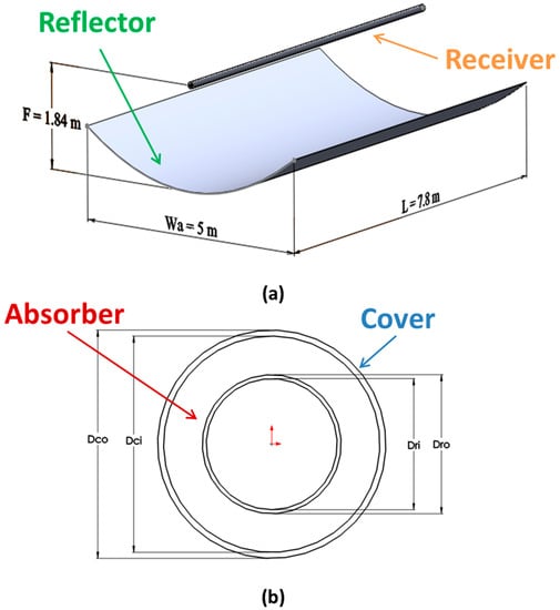
Figure 1.
(a) The examined module of the present analysis. (b) The main dimensions of the receiver.
Table 1 includes the main data of the examined PTC [31,32]. It is useful to state that the maximum optical efficiency, which is found for zero solar angle, it is about 75.3% by taking into consideration all the possible optical loss factors [32]. In this work, the solar angle is zero in all the cases and the ambient temperature is selected at 25 °C.

Table 1.
Data of the studied parabolic trough solar collector (PTC) module [31,32].
At this point, it is important to state that this work investigates a typical PTC module which has been studied by many other studies in the literature. So, the found results can be adopted as reliable also for other PTCs. More specifically, the present PTC has a typical evacuated receiver which is also used in other modules and it has a vacuum between the absorber and cover. Moreover, the collector is studied in a great range of usual operating conditions and so the found results are applicable in a great range of applications. Lastly, it has to be said that the used input properties (optical and thermal in Table 1) are usual and they correspond to real commercial systems. Therefore, the found results can be used also for other PTCs.
2.2. Basic Mathematical Formulation
The present section includes the main equations which have been used in the developed model in EES for the thermal efficiency determination of the PTC. The collector thermal efficiency (ηcol) is the ratio of useful heat production (Qu) to the solar energy on the collector aperture (Qs):
The solar irradiation in the collector aperture (Qs) can be written as:
The useful heat production (Qu) is calculated by the energy balance in the working fluid:
The inlet temperature (Tin), the outlet temperature (Tout), the oil mass flow rate (moil) and the oil specific heat capacity (cp) are used in the previous formula.
Moreover, the useful heat production (Qu) can be expressed as the heat that the absorber transfers to the working fluid:
The mean receiver temperature (Tr), the mean fluid temperature (Tfm), the internal tube area (Ari) and the convection heat transfer coefficient between fluid and absorber (h) are used in the previous formula.
The energy balance on the absorber is an important step in the present methodology and it is given below:
The absorbed solar energy (Qabs) can be found below:
The thermal losses (Qloss) of the absorber to the cover can be written as below [33]:
At this point, it has to be said that the convention thermal losses between absorber and cover are neglected due to the vacuum between them. Moreover, it is essential to state that the thermal losses from the absorber to the cover are the same as the losses from the cover to the ambient because the system is studied in steady-state conditions [33]. So, it can be said that:
The sky temperature (Tsky) can be estimated as below by using the temperature levels in kelvin units [34]:
The heat transfer coefficient between cover and ambient (hout) is found as below [35]:
More specifically, the wind speed (Vw) is selected at 1 m/s, which is a typical value, and the (hout) is found to be around 10 W/m2K [36].
The fluid flow heat transfer coefficient (h) is estimated by exploiting the Nusselt number (Nu):
The thermal conductive (k) of the thermal oil is dependent on the temperature and it is variable in this work [37].
For this work, the flow is turbulent (Re > 10,000) and there is a tubular channel. Thus, the formula of Dittus-Boelter about the Nusselt number can be used [38]:
The Reynolds number (Re) is defined as:
The Prandtl number (Pr) is defined as:
The mass flow rate (m) in (kg/s) is connected with the volumetric flow (V) in [L/min] as below:
In the end, it has to be said that the mean fluid temperature (Tfm) can be found as [39]:
2.3. Validation of the Developed Model in EES
The validation of the developed model in EES is performed by using experimental results by the literature [18]. Totally, 8 validation cases have been examined and they are depicted in Table 2. The inputs for every case are given on the left side of the table (Gb, Vw, Tam, Tin, V). Finally, Table 2 shows that the mean error about the outlet temperature is 1.22% and for the thermal efficiency of 1.68%. These are relatively low values which are in the range of the experimental errors. Thus, the developed model can be assumed as accurate for the present study.
Table 2.
Validation of the present model with experimental data from the Reference [18].
2.4. Followed Methodology for the Approximation Methods
In this work, the developed model in the Engineering Equation Solver (EES) [30] was applied in order to create a dataset for comparing the different formulas for the PTC thermal efficiency. EES is a flexible program for solving quickly and with accuracy numerous non-linear equations with numerical techniques [30]. It also includes libraries for using the thermal properties of different working fluids. Moreover, this program gives the possibility of conducting optimization studies for the maximization or the minimization of an objective function.
In this work, the solar irradiation (Gb) was examined from 300 W/m2 up to 1000 W/m2 with a step of 50 W/m2, while the inlet fluid temperature (Tin) from 25 °C up to 375 °C with a step of 50 °C. In this work, the temperature difference (ΔΤ = Τin − Τam) is important parameters which are examined from 0 °C up to 350 °C with a step of 50 °C, which is an equivalent parameter with the (Tin). The working fluid is Syltherm 800 which can operate up to 400 °C [37], something that has been taken into consideration in this work. The thermal properties of this fluid have been taken from the literature [37] and they are dependent on the fluid temperature level. Totally, 120 set points have been found and they are given in Appendix A.
About the solving procedures, for every case, the inputs in the program are the following: inlet temperature (Tin), oil flow volumetric rate (V), solar beam irradiation (Gb), ambient temperature (Tam), and the wind speed (Vw). Moreover, in this work, there is a zero-incident angle and so the optical efficiency has its maximum value according to Table 1. The program uses these inputs and calculates the outputs which are mainly the oil outlet temperature, the useful heat production, the thermal losses and the collector efficiency. The solution procedure is performed by combing the Equations (13) to (29) all together and by solving this system as a matrix with all the proper unknown parameters. Practically, it is a system with 17 equations and the following 17 unknown parameters: (ηcol), (Qu), (Qs), (Qabs), (Qloss), (Tout), (Tfm), (Tr), (Tc), (Tsky), (h), (hout), (Nu), (Re), (Pr), (m), (εr). The developed model in EES is solved iteratively in order for all these equations to be converged in the final values. Generally, the solution procedure is very quick with solving time lower than 1 s per case.
The literature review of this work indicates that the thermal efficiency of the PTC is expressed with polynomial expressions and thus, this strategy is investigated in this work in a detailed way. In this work, different polynomial formulas have been used in a systematic way. All these formulas can be expressed through the following general expression:
In all the examined cases, the constant term “a0” is included and all the proper combinations of the coefficients have been studied. In other words, every combination includes some parameters (e.g., a0, a1, a2, a3) and the other parameters are set to be zero (e.g., a4, b). In all the cases, there are at least two coefficients, the “a0” and another. The maximum number of the coefficients is six when all the coefficients are used in the approximation. The selection of the Formula (27) is in accordance with the existing literature. The term with “ΔΤ” is an important one, especially for the LS-2 module, and it has been used also in Reference [18]. The other terms are used in various studies. The maximum power is the fourth because the thermal radiation losses include this power and also there is no study in the literature with a higher power to be used. So, there is no reason for using the fifth power for example in the approximation formula because it would be unrealistic due to the radiation thermal losses law. So, this work studies the conventional polynomial expressions with the terms “ΔΤm/Gb” and for all the cases, the need for the extra term “ΔΤ” is evaluated. Finally, the goal is to determine the simplest expression which can lead to accurate results.
The approximation is conducted in every case with Microsoft Excel software and the command “linest”. The R2 is calculated as an effective index which has to be extremely close to 100%. Moreover, the mean absolute percentage error (MAPE) is an extra index that is calculated and it has to be close to zero. Its definition is given below:
where (n) is the total number of the dataset points which is equal to 120 in this work.
3. Results
3.1. Initial Analysis
The first part of this analysis is to investigate the relationship between thermal efficiency and the usually used parameters. Generally, the correlation of the thermal efficiency and the parameters “ΔΤm/Gb” (m = 1, 2, 3, 4) is suggested by the literature. Figure 2 shows these correlations, as well as the correlation between thermal efficiency and “ΔΤ”. The results are given for different solar beam irradiation levels and more specifically for 400, 600, 800 and 1000 W/m2. Figure 2a shows that there is not an important correlation between the thermal efficiency and the parameter “ΔΤ/Gb” because the curves are not all together but they have different trends for different solar irradiation levels. Similar results are found for Figure 2e with the parameter “ΔΤ” in the horizontal axis. Figure 2b shows that the curves are closer to each other, especially in low values of the parameter “ΔΤ2/Gb”, but it is not enough to describe the thermal efficiency with only the parameter “ΔΤ2/Gb”. However, the situation is different in Figure 2c,d for the parameters “ΔΤ3/Gb” and “ΔΤ4/Gb” respectively. More specifically, the curves are very close to each other when there is a plotting with the parameters “ΔΤ3/Gb” and “ΔΤ4/Gb” and especially in the case with “ΔΤ3/Gb”, which seems to be the best one. However, a deeper analysis is needed in order for the final conclusions to be extracted. In any case, it has been found that there is a need for using terms of high power and also there is a need for using more than one parameter in order to predict the thermal efficiency in an accurate way.

Figure 2.
Thermal efficiency as a function of different parameters: (a) ΔΤ/Gb, (b) ΔΤ2/Gb, (c) ΔΤ3/Gb, (d) ΔΤ4/Gb, (e) ΔΤ.
The next step is the detailed analysis of the correlation of the thermal efficiency with simple expressions of the format “a0 + am∙ΔTm/Gb” by using 120 operating points. Figure 3 depicts the obtained results. The valuation indexes (R2 and MAPE) are also included in these figures. The vertical axis is the value of the predicted efficiency while the horizontal axis shows the real value of the efficiency which has been calculated with EES. The results show that the use of the third power term leads to the best fitting and it is a very interesting result, which is in accordance with the quality conclusion from Figure 2. More specifically, for the formula “ΔΤ3/Gb”, the indexes are R2 = 99.11% and MAPE = 0.47%, while for “ΔΤ/Gb” they are R2 = 83.74% and MAPE = 1.85%, for “ΔΤ2/Gb” they are R2 = 97.74% and MAPE = 0.60% and for “ΔΤ4/Gb” they are R2 = 96.64% and MAPE = 0.93%. It is clear that the first power case leads to not acceptable results, while the powers of two and four lead to results with significant errors.

Figure 3.
Evaluation of the thermal efficiency equations of the form “a0 + am∙ΔTm/Gb” (a) [a0, a1] (b) [a0, a2] (c) [a0, a3] (d) [a0, a4]
The next step is to present approximation cases with the term “ΔΤ” to be included as an extra term to the previous studies’ formulas of Figure 3. So, Figure 4 exhibits the results about the use of the “a0 + am∙ΔTm/Gb + b∙ΔT” approximation about the thermal efficiency. Figure 4 indicates that the combination of the third power term with the temperature difference term leads to a very good fitting with R2 = 99.92% and MAPE = 0.13%. This high accuracy is obtained with only three parameters and this is a very interesting and promising result. Among the other cases of the “a0 + am∙ΔTm/Gb + b∙ΔT” formula, the use of the fourth power leads to R2 = 99.02%, which is an acceptable result, while the use of the power of two leads to R2 = 98.03%, which presents lower accuracy. Generally, when R2 is over 99% and the MAPE is lower than 0.50%, then the fitting can be evaluated as relatively accurate.

Figure 4.
Evaluation of the thermal efficiency equations of the form “a0 + am∙ΔTm/Gb + b∙ΔT” (a) [a0, a1, b] (b) [a0, a2, b] (c) [a0, a3, b] (d) [a0, a4, b].
To conclude, the use of the third power term leads to high accuracy, compared to the other cases, and especially when it is combined with the “ΔΤ” it leads to a very reliable model. In any case, the use of the extra term “ΔT” helps in all the cases and the expressions “a0 + am∙ΔTm/Gb + b∙ΔT” are more accurate than the respective “a0 + am∙ΔTm/Gb”, which is a reasonable result.
3.2. Total Analysis
The next stage of the present analysis is the investigation of more detailed approximation models with more terms. It is very interesting to see the approximation statistics with different linear combinations of the terms “am∙ΔTm/Gb” with and without the term “ΔΤ”. Figure 5 shows the results of the different linear combinations without the “ΔΤ”, while Figure 6 shows results with the term “ΔΤ”.
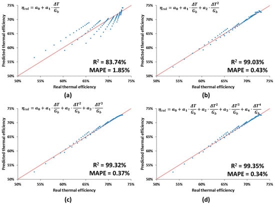
Figure 5.
Evaluation of the thermal efficiency equations of the form “a0 + ∑(am∙ΔTm/Gb)” (a) [a0, a1] (b) [a0, a1, a2] (c) [a0, a1, a2, a3] (d) [a0, a1, a2, a3, a4]

Figure 6.
Evaluation of the thermal efficiency equations of the form “a0 + ∑(am∙ΔTm/Gb) + b∙ΔT” (a) [a0, a1, b] (b) [a0, a1, a2, b] (c) [a0, a1, a2, a3, b] (d) [a0, a1, a2, a3, a4, b]
The general formula that is used in Figure 5 results can be written as “ηcol = a0 + ∑(am∙ΔTm/Gb)”. Figure 5 indicates that there is a need for using at least three terms in order for the points to be close to the red line and so to have a relatively accurate approximation. Also, the use of more terms leads to higher R2 and to lower MAPE, something that leads to better fitting. However, the difference between the cases with and without the term “ΔT4/Gb” is extremely low (R2 = 99.35% with this term and R2 = 99.32% without this term). This result indicates that there is a need for using the third-order term, while the fourth-order term has a very small impact on expression accuracy.
The next step is the implementation of the extra term “ΔΤ” in the previous expressions and so the general formula is “ηcol = a0 + ∑(am∙ΔTm/Gb) + b∙ΔΤ”. Figure 6 indicates that the use of this term leads to very accurate models for all the cases except the case with the first-order term “ΔT/Gb”, where the R2 is only 87.45%. The cases with the order with m = 2, m = 3 and m = 4 lead to R2 at 99.44%, 99.94% and 99.94%, respectively. The MAPE is found to be found 1.69%, 0.37%, 0.12% and 0.11% for the cases with m = 1, m = 2, m = 3 and m = 4, respectively. Practically, the use of the fourth power term is useless because it leads to approximately the same results with the third term results.
To conclude about the results of Figure 5 and Figure 6, the use of the third-order term is very important and also the use of the “ΔΤ” is a very useful weapon for the proper prediction of the PTC thermal efficiency.
The next step in this analysis is to present all the results about the coefficients of approximation and the evaluation indexes about the 31 examined cases. Table 3 includes all these data and this table summarizes all the found results of this work. In this table, the 31 different approximations are included. The evaluation indexes (R2 and MAPE), as well as the values of the coefficients (a0, a1, a2, a4, b) are given. In the cases with empty cells, there is no utilization of the respective term and so the empty cells indicate that the respective value is zero.
Table 3.
Evaluation indexes for the examined formulas (The empty cells indicate that the respective term is not taken into account and the bold lines indicate the best cases).
In the left column of Table 3, the number terms of the used formulas are given and the equations are classified in categories with 2 to 6 terms. Among the equations with two terms, the best formula is the following:
Equation (29) is a very simple formula that leads to relatively accurate results and it is a promising choice. So, the use of the third power term seems to be a very good idea for the proper approximation of the PTC performance.
In the equations family with three terms, the best fitting has been found for the following formula:
Equation (30) includes the constant term, the third-order term and the term about the temperature difference. There is an excellent fitting with Equation (30) which leads to R2 = 99.92% and MAPE = 0.13%. These results can be compared with the indexes about Equation (29) which does not include the term “ΔΤ”, where R2 = 99.11% and MAPE = 0.47%. There is a significant difference that can be obtained only by adding an extra term. This result indicates that the use of the term “ΔΤ” is an important one in the efficiency approximation study.
About the studies with four terms, practically all the formulas lead to good fitting. Generally, the cases with third-order terms and “ΔΤ” again lead to accurate fitting. For the case with four terms, the best fitting is given below:
About the cases with 5 and 6 terms, the fittings are excellent. Below, the formula with the six terms, which includes all the used parameters, is given:
It is very interesting to state that the use of some extra terms maybe cannot increase the accuracy effectively. Comparing Equations (30) and (32), the difference between the indexes is marginal, while Equation (30) uses 3 terms and Equation (32) uses 6 terms. So, it can be said that there is great importance to the proper term selection in order to have an accurate approximation.
Moreover, it can be said that the use of more and more terms is not the only choice for having more accurate results because the computational cost and the complexity of the approximation increase without a significant increase in the fitting suitability. A characteristic example is a comparison of the Formula (30), which includes the terms (a0, a3, b) with the formula which includes the terms (a0, a1, a2, a3, a4). According to Table 3, the first one with 3 terms has R2 = 99.92%, while the other one with 5 terms has R2 = 99.35%. So, it is obvious that the increase in the number of terms and the power of the terms is not the proper choice for a good fitting. So, it is suggested to use terms with third-order power and the terms with “ΔΤ”.
In the literature, the use of the term “ΔΤ” is not unknown and it has been used in some studies, with the most characteristic approximation of experimental results about LS-2 PTC by Dudley et al. [18]. They applied a model with (a0, a1, a2, b) in order to have a proper fitting. The fitting of this expression, in the present example, leads to R2 = 99.44%, which is acceptable but is lower than the respective of Equation (30) with the terms model (a0, a3, b) which is 99.92%.
Another important result of this work is the determination of the third-order as the most proper one, especially in cases with a small number of terms. This result is not found in the existing literature. Usually, second or four power terms are used. Characteristic examples are the studies of References [24,25,26], where the only not-studied term is the one with the third power. This note proves that there is a scientific gap that is covered by the present work.
Another interesting comparison of the suggested model (a0, a3, b) is with the steady-state models that are suggested by the IEC 62862-3-2. Practically, the polynomial terms of this standard are taken into consideration in order to compare them with the existing optimum model. The use of the second-order terms, of the forth-order term and their combination is compared with the third-order term. The present model presents R2 = 99.92% and MAPE = 0.13%, while the other models of the standard have not so good fitting. More specifically, the (a0, a1, a2) model has R2 = 99.03% and MAPE = 0.43%, the (a0, a1, a4) has R2 = 98.96% and MAPE = 0.48% and the (a0, a1, a2, a4) has R2 = 99.33% and MAPE = 0.35%. So, it can be said that the suggested model is a promising one for approximating the PTC thermal efficiency. However, it has to be said that the other models are also accurate models and their use leads to an efficient approximation of the thermal efficiency data. In order to give a clear image of the aforementioned comparison, Figure 7 has been added in order to directly compare the model (a0, a3, b) with the models (a0, a1, a2), (a0, a1, a4) and (a0, a1, a2, a4). In this figure, the results from the ESS for Gb = 1000 W/m2 are plotted with the found curves for the three models. It can be said that the model (a0, a3, b) is close to the found points while the other models present some deviations especially in low and high values of (ΔΤ).

Figure 7.
Comparison of the suggested model (a0, a3, b) with other usual models for Gb = 1000 W/m2.
In the future, there is a need for performing similar detailed and systematic approximating studies by taking into account the wind speed (especially for bare tube cases), the solar angle (through the incident angle modifier) and the flow rate. Moreover, studies about different PTCs with a non-evacuated tube, non-selective absorber, different concentration ratios, different working fluid and different materials can also be studied.
4. Conclusions
The objective of this work was to investigate different mathematical expressions for the determination of thermal efficiency in a parabolic trough solar collector (PTC). A detailed literature review was conducted in order to highlight what are the usual expressions in the existing literature. This work examined 31 different models which are specific cases of a generalized formula. A numerical model about the thermal efficiency of the PTC was developed and it has been validated by literature experimental data. This model regards the LS-2 PTC module which is a usual module that is used in studies about PTC and the respective applications. The results of this work can be extended and applied for all the PTC modules and not only for the examined one because the usual PTC characteristics have been selected. Below, the most important conclusions are given:
- -
- The use of the third-order term “ΔΤ3/Gb” is the most important term which can lead to relatively accurate results, especially in cases with a low number of terms.
- -
- The use of the temperature difference term “ΔΤ” is important and it can lead to high improvement compared to the respective formulas without it.
- -
- The most promising formula by taking into account the use of a low number of parameters and to achieve high accuracy is the following:, (R2 = 99.92% – MAPE = 0.13%) or in a general form:
- -
- It is found and discussed that there is a need for using the proper terms and not using many terms in order to achieve high accuracy.
- -
- In the future, there is a need for extending the present work by taking into consideration the wind speed, the solar angle and the flow rate. Moreover, there is a need for studying extra PTC modules with different characteristics than the present one, for example with a non-selective absorber, with a non-evacuated receiver and with different working fluid.
Author Contributions
E.B. conceptualization, methodology, investigation, writing—review and editing, writing—original draft preparation; C.T. supervision, writing—review and editing, writing—original draft preparation. All authors have read and agreed to the published version of the manuscript.
Funding
This research received no external funding.
Conflicts of Interest
The authors declare no conflict of interest.
Nomenclature
| A | Area, m2 |
| αi | Approximation coefficient (i = 0, 1, 2, 3, 4) |
| b | Approximation coefficient, K−1 |
| ci | Approximation coefficient (i = 0, 1, 2, 3, 4) |
| C | Concentration ratio |
| cp | Specific heat capacity under constant pressure, J kg−1 K−1 |
| D | Diameter, m |
| EL | Longwave irradiance, W m−2 |
| F | Focal distance, m |
| Gb | Solar direct beam irradiation, W m−2 |
| h | Heat transfer coefficient of the flow, W m−2 K−1 |
| hout | Convection coefficient between cover and ambient, W m−2 K−1 |
| i | Counter |
| k | Thermal conductivity, W m−1 K−1 |
| L | Tube length, m |
| m | Power of the approximation term |
| moil | Thermal oil mass flow rate, kg s−1 |
| n | Number of the examined scenarios |
| Nu | Nusselt number |
| Pr | Prandtl number |
| Q | Heat rate, W |
| Re | Reynolds number |
| R2 | Coefficient of determination |
| T | Temperature, °C |
| Tsky | Sky temperature, K |
| V | Volumetric flow rate, L min−1 |
| Vw | Wind speed, m s−1 |
| Wa | Width, m |
| Greek symbols | |
| α | Absorbance |
| γ | Intercept factor |
| ΔΤ | Temperature difference [= Tin − Tam], °C |
| ε | Emittance |
| ηcol | Collector thermal efficiency |
| ηopt | Optical efficiency |
| θ | Solar incident angle, ° |
| μ | Dynamic Viscosity, Pa s |
| ρ | Equivalent reflectance |
| σ | Stefan-Boltzmann constant [= 5.67 ∙ 10−8 W m−2 K−4] |
| τ | Transmittance |
| Subscripts and superscripts | |
| a | aperture |
| am | ambient |
| aprx | approximation |
| b | beam |
| c | cover |
| ci | cover inner |
| co | outer cover |
| d | diffuse |
| fm | mean fluid |
| in | inlet |
| m | power of the approximation term |
| max | maximum |
| out | outlet |
| r | receiver |
| ri | inner receiver |
| ro | receiver outer |
| s | solar |
| u | useful |
Abbreviations
| EES | Engineering equation solver |
| MAPE | Mean absolute percentage error |
| PTC | Parabolic trough collector |
Appendix A—Dataset for the Present Work
Appendix A includes the dataset for the approximation studies which have been found by the use of the EES model. Table A1 includes the inlet temperatures (Tin), the solar irradiation (Gb), the temperature difference (ΔΤ = Τin − Tam) and the collector thermal efficiency (ηcol). It has to be said that these points have been found for ambient temperature (Tam) at 25 °C, volumetric flow rate (V) of 100 L/min, wind speed (Vw) at 1 m/s and zero solar angle (θ).
Moreover, the thermal efficiency with three approximation formulas is given in Table A1. The three examined formulas, which have high interest, are given below with the numbering (A1), (A2) and (A3):
So, Table A1 shows the “reference” values from the EES model and the approximation with three other models in order to make clear how close the efficiency is found with these three important models.
Table A1.
Dataset for the approximation studies.
Table A1.
Dataset for the approximation studies.
| Tin (°C) | ΔΤ (°C) | Gb (W/m2) | ηcol | |||
|---|---|---|---|---|---|---|
| EES | Equation (A1) | Equation (A2) | Equation (A3) | |||
| 25 | 0 | 1000 | 0.73056 | 0.72547 | 0.73116 | 0.73187 |
| 75 | 50 | 1000 | 0.72885 | 0.72530 | 0.72831 | 0.72876 |
| 125 | 100 | 1000 | 0.72550 | 0.72406 | 0.72452 | 0.72461 |
| 175 | 150 | 1000 | 0.72007 | 0.72070 | 0.71887 | 0.71883 |
| 225 | 200 | 1000 | 0.71183 | 0.71415 | 0.71044 | 0.71060 |
| 275 | 250 | 1000 | 0.69965 | 0.70336 | 0.69828 | 0.69886 |
| 325 | 300 | 1000 | 0.68187 | 0.68726 | 0.68147 | 0.68237 |
| 375 | 350 | 1000 | 0.65670 | 0.66479 | 0.65909 | 0.65966 |
| 25 | 0 | 950 | 0.73067 | 0.72547 | 0.73116 | 0.73187 |
| 75 | 50 | 950 | 0.72886 | 0.72529 | 0.72830 | 0.72873 |
| 125 | 100 | 950 | 0.72540 | 0.72398 | 0.72446 | 0.72451 |
| 175 | 150 | 950 | 0.71979 | 0.72044 | 0.71865 | 0.71856 |
| 225 | 200 | 950 | 0.71125 | 0.71355 | 0.70992 | 0.71003 |
| 275 | 250 | 950 | 0.69862 | 0.70219 | 0.69726 | 0.69781 |
| 325 | 300 | 950 | 0.68021 | 0.68524 | 0.67971 | 0.68060 |
| 375 | 350 | 950 | 0.65412 | 0.66159 | 0.65629 | 0.65682 |
| 25 | 0 | 900 | 0.73076 | 0.72547 | 0.73116 | 0.73187 |
| 75 | 50 | 900 | 0.72887 | 0.72528 | 0.72829 | 0.72870 |
| 125 | 100 | 900 | 0.72528 | 0.72390 | 0.72438 | 0.72439 |
| 175 | 150 | 900 | 0.71946 | 0.72017 | 0.71841 | 0.71826 |
| 225 | 200 | 900 | 0.71060 | 0.71289 | 0.70934 | 0.70940 |
| 275 | 250 | 900 | 0.69748 | 0.70090 | 0.69613 | 0.69665 |
| 325 | 300 | 900 | 0.67834 | 0.68301 | 0.67775 | 0.67862 |
| 375 | 350 | 900 | 0.65124 | 0.65804 | 0.65318 | 0.65367 |
| 25 | 0 | 850 | 0.73086 | 0.72547 | 0.73116 | 0.73187 |
| 75 | 50 | 850 | 0.72886 | 0.72526 | 0.72828 | 0.72867 |
| 125 | 100 | 850 | 0.72513 | 0.72381 | 0.72430 | 0.72426 |
| 175 | 150 | 850 | 0.71908 | 0.71985 | 0.71814 | 0.71792 |
| 225 | 200 | 850 | 0.70986 | 0.71215 | 0.70869 | 0.70869 |
| 275 | 250 | 850 | 0.69618 | 0.69945 | 0.69486 | 0.69535 |
| 325 | 300 | 850 | 0.67623 | 0.68051 | 0.67556 | 0.67641 |
| 375 | 350 | 850 | 0.64799 | 0.65408 | 0.64970 | 0.65015 |
| 25 | 0 | 800 | 0.73095 | 0.72547 | 0.73116 | 0.73187 |
| 75 | 50 | 800 | 0.72884 | 0.72525 | 0.72827 | 0.72863 |
| 125 | 100 | 800 | 0.72496 | 0.72370 | 0.72421 | 0.72411 |
| 175 | 150 | 800 | 0.71865 | 0.71950 | 0.71783 | 0.71754 |
| 225 | 200 | 800 | 0.70901 | 0.71132 | 0.70796 | 0.70790 |
| 275 | 250 | 800 | 0.69470 | 0.69783 | 0.69344 | 0.69388 |
| 325 | 300 | 800 | 0.67384 | 0.67770 | 0.67310 | 0.67393 |
| 375 | 350 | 800 | 0.64432 | 0.64961 | 0.64579 | 0.64619 |
| 25 | 0 | 750 | 0.73104 | 0.72547 | 0.73116 | 0.73187 |
| 75 | 50 | 750 | 0.72881 | 0.72524 | 0.72825 | 0.72859 |
| 125 | 100 | 750 | 0.72474 | 0.72359 | 0.72411 | 0.72394 |
| 175 | 150 | 750 | 0.71814 | 0.71910 | 0.71748 | 0.71710 |
| 225 | 200 | 750 | 0.70803 | 0.71037 | 0.70713 | 0.70700 |
| 275 | 250 | 750 | 0.69301 | 0.69598 | 0.69182 | 0.69222 |
| 325 | 300 | 750 | 0.67111 | 0.67452 | 0.67031 | 0.67111 |
| 375 | 350 | 750 | 0.64012 | 0.64456 | 0.64136 | 0.64170 |
| 25 | 0 | 700 | 0.73112 | 0.72547 | 0.73116 | 0.73187 |
| 75 | 50 | 700 | 0.72876 | 0.72522 | 0.72824 | 0.72854 |
| 125 | 100 | 700 | 0.72449 | 0.72345 | 0.72399 | 0.72375 |
| 175 | 150 | 700 | 0.71755 | 0.71865 | 0.71708 | 0.71661 |
| 225 | 200 | 700 | 0.70690 | 0.70930 | 0.70619 | 0.70597 |
| 275 | 250 | 700 | 0.69106 | 0.69388 | 0.68998 | 0.69033 |
| 325 | 300 | 700 | 0.66797 | 0.67088 | 0.66712 | 0.66790 |
| 375 | 350 | 700 | 0.63530 | 0.63878 | 0.63630 | 0.63656 |
| 25 | 0 | 650 | 0.73120 | 0.72547 | 0.73116 | 0.73187 |
| 75 | 50 | 650 | 0.72870 | 0.72520 | 0.72822 | 0.72849 |
| 125 | 100 | 650 | 0.72418 | 0.72330 | 0.72385 | 0.72352 |
| 175 | 150 | 650 | 0.71685 | 0.71812 | 0.71662 | 0.71604 |
| 225 | 200 | 650 | 0.70558 | 0.70805 | 0.70510 | 0.70478 |
| 275 | 250 | 650 | 0.68880 | 0.69145 | 0.68785 | 0.68814 |
| 325 | 300 | 650 | 0.66433 | 0.66668 | 0.66344 | 0.66418 |
| 375 | 350 | 650 | 0.62971 | 0.63211 | 0.63045 | 0.63064 |
| 25 | 0 | 600 | 0.73127 | 0.72547 | 0.73116 | 0.73187 |
| 75 | 50 | 600 | 0.72860 | 0.72518 | 0.72820 | 0.72843 |
| 125 | 100 | 600 | 0.72381 | 0.72311 | 0.72369 | 0.72326 |
| 175 | 150 | 600 | 0.71602 | 0.71751 | 0.71608 | 0.71538 |
| 225 | 200 | 600 | 0.70402 | 0.70660 | 0.70382 | 0.70340 |
| 275 | 250 | 600 | 0.68613 | 0.68861 | 0.68536 | 0.68559 |
| 325 | 300 | 600 | 0.66005 | 0.66178 | 0.65915 | 0.65985 |
| 375 | 350 | 600 | 0.62316 | 0.62433 | 0.62364 | 0.62373 |
| 25 | 0 | 550 | 0.73135 | 0.72547 | 0.73116 | 0.73187 |
| 75 | 50 | 550 | 0.72848 | 0.72515 | 0.72818 | 0.72835 |
| 125 | 100 | 550 | 0.72336 | 0.72290 | 0.72351 | 0.72296 |
| 175 | 150 | 550 | 0.71502 | 0.71679 | 0.71545 | 0.71459 |
| 225 | 200 | 550 | 0.70217 | 0.70488 | 0.70232 | 0.70176 |
| 275 | 250 | 550 | 0.68296 | 0.68526 | 0.68243 | 0.68257 |
| 325 | 300 | 550 | 0.65496 | 0.65599 | 0.65408 | 0.65473 |
| 375 | 350 | 550 | 0.61538 | 0.61513 | 0.61558 | 0.61557 |
| 25 | 0 | 500 | 0.73141 | 0.72547 | 0.73116 | 0.73187 |
| 75 | 50 | 500 | 0.72831 | 0.72512 | 0.72815 | 0.72826 |
| 125 | 100 | 500 | 0.72280 | 0.72264 | 0.72328 | 0.72259 |
| 175 | 150 | 500 | 0.71381 | 0.71592 | 0.71469 | 0.71365 |
| 225 | 200 | 500 | 0.69992 | 0.70283 | 0.70052 | 0.69980 |
| 275 | 250 | 500 | 0.67914 | 0.68124 | 0.67890 | 0.67895 |
| 325 | 300 | 500 | 0.64884 | 0.64904 | 0.64799 | 0.64859 |
| 375 | 350 | 500 | 0.60600 | 0.60410 | 0.60591 | 0.60577 |
| 25 | 0 | 450 | 0.73148 | 0.72547 | 0.73116 | 0.73187 |
| 75 | 50 | 450 | 0.72810 | 0.72508 | 0.72812 | 0.72815 |
| 125 | 100 | 450 | 0.72210 | 0.72233 | 0.72300 | 0.72214 |
| 175 | 150 | 450 | 0.71231 | 0.71486 | 0.71376 | 0.71250 |
| 225 | 200 | 450 | 0.69715 | 0.70031 | 0.69831 | 0.69740 |
| 275 | 250 | 450 | 0.67444 | 0.67633 | 0.67460 | 0.67452 |
| 325 | 300 | 450 | 0.64132 | 0.64055 | 0.64055 | 0.64108 |
| 375 | 350 | 450 | 0.59451 | 0.59061 | 0.59410 | 0.59380 |
| 25 | 0 | 400 | 0.73153 | 0.72547 | 0.73116 | 0.73187 |
| 75 | 50 | 400 | 0.72780 | 0.72503 | 0.72807 | 0.72801 |
| 125 | 100 | 400 | 0.72121 | 0.72193 | 0.72266 | 0.72158 |
| 175 | 150 | 400 | 0.71042 | 0.71353 | 0.71260 | 0.71106 |
| 225 | 200 | 400 | 0.69366 | 0.69716 | 0.69556 | 0.69440 |
| 275 | 250 | 400 | 0.66853 | 0.67018 | 0.66921 | 0.66899 |
| 325 | 300 | 400 | 0.63188 | 0.62993 | 0.63125 | 0.63170 |
| 375 | 350 | 400 | 0.58009 | 0.57375 | 0.57933 | 0.57883 |
| 25 | 0 | 350 | 0.73158 | 0.72547 | 0.73116 | 0.73187 |
| 75 | 50 | 350 | 0.72741 | 0.72497 | 0.72802 | 0.72784 |
| 125 | 100 | 350 | 0.72005 | 0.72143 | 0.72222 | 0.72086 |
| 175 | 150 | 350 | 0.70796 | 0.71182 | 0.71110 | 0.70921 |
| 225 | 200 | 350 | 0.68915 | 0.69312 | 0.69201 | 0.69054 |
| 275 | 250 | 350 | 0.66091 | 0.66228 | 0.66229 | 0.66188 |
| 325 | 300 | 350 | 0.61971 | 0.61628 | 0.61929 | 0.61963 |
| 375 | 350 | 350 | 0.56150 | 0.55208 | 0.56034 | 0.55959 |
| 25 | 0 | 300 | 0.73161 | 0.72547 | 0.73116 | 0.73187 |
| 75 | 50 | 300 | 0.72686 | 0.72488 | 0.72794 | 0.72760 |
| 125 | 100 | 300 | 0.71847 | 0.72075 | 0.72163 | 0.71990 |
| 175 | 150 | 300 | 0.70466 | 0.70955 | 0.70911 | 0.70674 |
| 225 | 200 | 300 | 0.68311 | 0.68773 | 0.68729 | 0.68540 |
| 275 | 250 | 300 | 0.65071 | 0.65175 | 0.65307 | 0.65240 |
| 325 | 300 | 300 | 0.60343 | 0.59808 | 0.60334 | 0.60355 |
| 375 | 350 | 300 | 0.53665 | 0.52318 | 0.53502 | 0.53393 |
References
- Bellos, E.; Tzivanidis, C. Alternative designs of parabolic trough solar collectors. Prog. Energy Combust. Sci. 2019, 71, 81–117. [Google Scholar] [CrossRef]
- Shahverdi, K.; Loni, R.; Ghobadian, B.; Monem, M.J.; Gohari, S.; Marofi, S.; Najafi, G. Energy harvesting using solar ORC system and Archimedes Screw Turbine (AST) combination with different refrigerant working fluids. Energy Convers. Manag. 2019, 187, 205–220. [Google Scholar] [CrossRef]
- Silva, R.; Berenguel, M.; García, M.P.; Fernández-García, A. Thermo-economic design optimization of parabolic trough solar plants for industrial process heat applications with memetic algorithms. Appl. Energy 2014, 113, 603–614. [Google Scholar] [CrossRef]
- Cabrera, F.; Fernández-García, A.; Silva, R.; García, M.P. Use of parabolic trough solar collectors for solar refrigeration and air-conditioning applications. Renew. Sustain. Energy Rev. 2013, 20, 103–118. [Google Scholar] [CrossRef]
- Tian, Z.; Perers, B.; Furbo, S.; Fan, J. Thermo-economic optimization of a hybrid solar district heating plant with flat plate collectors and parabolic trough collectors in series. Energy Convers. Manag. 2018, 165, 92–101. [Google Scholar] [CrossRef]
- Mosaffa, A.; Ghaffarpour, Z.; Farshi, L.G. Thermoeconomic assessment of a novel integrated CHP system incorporating solar energy based biogas-steam reformer with methanol and hydrogen production. Sol. Energy 2019, 178, 1–16. [Google Scholar] [CrossRef]
- Kasaeian, A.; Bellos, E.; Shamaeizadeh, A.; Tzivanidis, C. Solar-driven polygeneration systems: Recent progress and outlook. Appl. Energy 2020, 264, 114764. [Google Scholar] [CrossRef]
- Kumar, A.; Sharma, M.; Thakur, P.; Thakur, V.; Rahatekar, S.; Kumar, R. A review on exergy analysis of solar parabolic collectors. Sol. Energy 2020, 197, 411–432. [Google Scholar] [CrossRef]
- Bellos, E.; Tzivanidis, C.; Tsimpoukis, D. Thermal, hydraulic and exergetic evaluation of a parabolic trough collector operating with thermal oil and molten salt based nanofluids. Energy Convers. Manag. 2018, 156, 388–402. [Google Scholar] [CrossRef]
- Xu, H.; Li, Y.; Sun, J.; Li, L. Transient model and characteristics of parabolic-trough solar collectors: Molten salt vs. synthetic oil. Sol. Energy 2019, 182, 182–193. [Google Scholar] [CrossRef]
- Bellos, E.; Tzivanidis, C.; Antonopoulos, K.A.; Daniil, I. The use of gas working fluids in parabolic trough collectors—An energetic and exergetic analysis. Appl. Therm. Eng. 2016, 109A, 1–14. [Google Scholar] [CrossRef]
- Kalogirou, S. Parabolic trough collector system for low temperature steam generation: Design and performance characteristics. Appl. Energy 1996, 55, 1–19. [Google Scholar] [CrossRef]
- Coccia, G.; Di Nicola, G.; Sotte, M. Design, manufacture, and test of a prototype for a parabolic trough collector for industrial process heat. Renew. Energy 2015, 74, 727–736. [Google Scholar] [CrossRef]
- Duffie, J.A.; Beckman, W.A. Solar Engineering of Thermal Processes, 2nd ed.; Wiley: New York, NY, USA, 1991. [Google Scholar]
- ISO. Standard 9806-1: Test Methods for Solar Collectors. Part 1: Thermal Performance of Liquid Heating Collectors Including Pressure Drop; ISO: Geneva, Switzerland, 1994. [Google Scholar]
- Bellos, E.; Tzivanidis, C.; Belessiotis, V. Daily performance of parabolic trough solar collectors. Sol. Energy 2017, 158, 663–678. [Google Scholar] [CrossRef]
- Kalogirou, S.A.; Panayiotou, G. Evaluation of a Parabolic Trough Collector Performance. In Proceedings of the World Renewable Energy Forum, WREF 2012, Including World Renewable Energy Congress XII and Colorado Renewable Energy Society (CRES) Annual Conference, Denver, CO, USA, 13–17 May 2012; Volume 3, pp. 2085–2091. [Google Scholar]
- Dudley, V.; Kolb, G.; Sloan, M.; Kearney, D. SEGS LS2 Solar Collector-Test Results, Report of Sandia National Laboratories, SAN94-1884; Sandia National Laboratories: Albuquerque, NM, USA, 1994. [Google Scholar]
- Kutscher, C.; Burkholder, F.; Stynes, J.K. Generation of a Parabolic Trough Collector Efficiency Curve From Separate Measurements of Outdoor Optical Efficiency and Indoor Receiver Heat Loss. J. Sol. Energy Eng. 2011, 134, 011012. [Google Scholar] [CrossRef]
- Nemś, M.; Kasperski, J. Determining non-linear characteristics of a concentrating solar collector according to the experiment design. J. Phys. Conf. Ser. 2016, 745, 032107. [Google Scholar] [CrossRef]
- Sallaberry, F.; Bello, A.; Burgaleta, J.I.; Fernández-García, A.; Fernández-Reche, J.; Gomez, J.A.; Herrero, S.; Lüpfert, E.; Morillo, R.; Vicente, G.S.; et al. Standards for components in concentrating solar thermal power plants—Status of the Spanish working group. In Proceedings of the SOLARPACES 2015: International Conference on Concentrating Solar Power and Chemical Energy Systems, Cape Town, South Africa, 13–16 October 2015; AIP Publishing: University Park City, MA, USA, 2016; Volume 1734, p. 110003. [Google Scholar]
- IEC. IEC 62817, Solar Trackers for Photovoltaic Systems—Design Qualification; IEC: Geneva, Switzerland, 2014. [Google Scholar]
- Odeh, S.D.; Morrison, G.L.; Behnia, M. Thermal analysis of parabolic trough solar collectors for electric power generation. In Proceedings of the ANZSES Annual Conference, Darwin, Australia, 22–25 October 1996; pp. 460–467. [Google Scholar]
- Sallaberry, F.; Valenzuela, L.; Palacin, L.G.; Leon, J.; Fischer, S.; Bohren, A. Harmonization of standards for parabolic trough collector testing in solar thermal power plants. In Proceedings of the SOLARPACES 2016: International Conference on Concentrating Solar Power and Chemical Energy Systems, Abu Dhabi, The United Arab Emirates, 11–14 October 2016; AIP Publishing: University Park, MA, USA, 2017; Volume 1850, p. 20014. [Google Scholar]
- Sallaberry, F.; Valenzuela, L.; Palacin, L.G. On-site parabolic-trough collector testing in solar thermal power plants: Experimental validation of a new approach developed for the IEC 62862-3-2 standard. Sol. Energy 2017, 155, 398–409. [Google Scholar] [CrossRef]
- ISO. DIS/ISO 9806 Standard Draft Solar Energy—Test Method for Solar Collectors; ISO: Geneva, Switzerland, 2017. [Google Scholar]
- Xu, L.; Wang, Z.; Li, X.; Yuan, G.; Sun, F.; Lei, D.; Li, S. A comparison of three test methods for determining the thermal performance of parabolic trough solar collectors. Sol. Energy 2014, 99, 11–27. [Google Scholar] [CrossRef]
- Bellos, E.; Tzivanidis, C. Analytical Expression of Parabolic Trough Solar Collector Performance. Designs 2018, 2, 9. [Google Scholar] [CrossRef]
- Lüpfert, E.; Herrmann, U.; Price, H.; Zarza, E.; Kistner, R. Towards standard performance analysis for parabolic trough collector fields. In Proceedings of the SolarPaces Conference, Oaxaca, Mexico, 6–9 September 2004. [Google Scholar]
- F-Chart Software, Engineering Equation Solver (EES). 2015. Available online: http://www.fchart.com/ees (accessed on 23 August 2020).
- Forristall, R. Heat Transfer Analysis and Modeling of a Parabolic Trough Solar Receiver Implemented in Engineering Equation Solver; National Renewable Energy Laboratory (NREL): Golden, CO, USA, 2003. [Google Scholar]
- Behar, O.; Khellaf, A.; Mohammedi, K. A novel parabolic trough solar collector model—Validation with experimental data and comparison to Engineering Equation Solver (EES). Energy Convers. Manag. 2015, 106, 268–281. [Google Scholar] [CrossRef]
- Tzivanidis, C.; Bellos, E.; Korres, D.; Antonopoulos, K.; Mitsopoulos, G. Thermal and optical efficiency investigation of a parabolic trough collector. Case Stud. Therm. Eng. 2015, 6, 226–237. [Google Scholar] [CrossRef]
- Swinbank, W.C. Long-wave radiation from clear skies. Q. J. R. Meteorol. Soc. 1963, 89, 339–348. [Google Scholar] [CrossRef]
- Bhowmik, N.; Mullick, S. Calculation of tubular absorber heat loss factor. Sol. Energy 1985, 35, 219–225. [Google Scholar] [CrossRef]
- Bellos, E.; Tzivanidis, C.; Tsimpoukis, D. Enhancing the performance of parabolic trough collectors using nanofluids and turbulators. Renew. Sustain. Energy Rev. 2018, 91, 358–375. [Google Scholar] [CrossRef]
- SYLTHERM 800 Heat Transfer Fluid. Available online: https://www.dow.com/content/dam/dcc/documents/en-us/app-tech-guide/176/176-01435-01-syltherm-800-heat-transfer-fluid.pdf?iframe=true (accessed on 23 August 2020).
- Leinhard, J., IV; Leinhard, J., V. A Heat Tranfer Textbook, 4th ed.; Philogiston Press: Cambridge, MA, USA, 2012. [Google Scholar]
- Bellos, E.; Tzivanidis, C.; Tsimpoukis, D. Optimum number of internal fins in parabolic trough collectors. Appl. Therm. Eng. 2018, 137, 669–677. [Google Scholar] [CrossRef]


© 2020 by the authors. Licensee MDPI, Basel, Switzerland. This article is an open access article distributed under the terms and conditions of the Creative Commons Attribution (CC BY) license (http://creativecommons.org/licenses/by/4.0/).