A Fuzzy Markov Model for Risk and Reliability Prediction of Engineering Systems: A Case Study of a Subsea Wellhead Connector

Featured Application

The reliability of many engineering systems (such as offshore and subsea equipment, aerospace equipment, energy production equipment, etc.) is very important, but due to a lack of sufficient failure data, their reliability is difficult to accurately evaluate. If the data is obtained through experiments, it will consume a huge amount of money, manpower and time, and there is no suitable experiment to perform an accurate simulation. The method in this paper completely solves this problem. The method proposed in this paper can not only obtain accurate reliability and availability, but also evaluate the impact of uncertain events on system reliability during equipment operation.

Abstract

In production environments, failure data of a complex system are difficult to obtain due to the high cost of experiments; furthermore, using a single model to analyze risk, reliability, availability and uncertainty is a big challenge. Based on the fault tree, fuzzy comprehensive evaluation and Markov method, this paper proposed a fuzzy Markov method that takes the full advantages of the three methods and makes the analysis of risk, reliability, availability and uncertainty all in one. This method uses the fault tree and fuzzy theory to preprocess the input failure data to improve the reliability of the input failure data, and then input the preprocessed failure data into the Markov model; after that iterate and adjust the model when uncertainty events occur, until the data of all events have been processed by the model and the updated model obtained, which best reflects the system state. The wellhead connector of a subsea production system was used as a case study to demonstrate the above method. The obtained reliability index (mean time to failure) of the connector is basically consistent with the failure statistical data from the offshore and onshore reliability database, which verified the accuracy of the proposed method.

1. Introduction

Many engineering systems have such characters as high technology, high investment and high risk. During the operation process, the complex system is enormously affected by the internal and external loads, such as vibration, fatigue, temperature and human operation factors, even subjected to various hazards including natural disasters, terrorist and criminal acts [1,2,3]. Once an accident occurs, it will cause a series of problems such as transport accidents, explosions, casualties, fires and chemical and biological emission. Especially equipment storing inflammable and explosive materials such as chemical fuels, aviation equipment that is extremely hazardous in the event of an accident, and facilities that transport oil and gas energy have negative effects on environment, economy, society and life if an accident happened. Therefore, good judgments should be made on the risk, reliability, availability and uncertainty of such facilities.

A series of analysis methods were proposed over the years for reliability and risk evaluation, such as fault tree, bowtie, event tree, Petri nets, Markov models, Bayesian networks and so on. Though these methods can model potential faults, they have limited capabilities to handle insufficient data of failure probabilities, therefore resulting in an inaccurate risk assessment result [4]. To resolve this issue, expert evaluation and fuzzy theory were adopted to calculate fuzzy failure probabilities of risk factors. The method can characterize the uncertain parameters involved in a risk analysis process [2,5]. The method has been extensively used in engineering fields, such as aerospace, subsea facilities, energy, transport, etc. Mentes introduced it into fault tree to calculate probabilities of base events of spread mooring systems [6]. Babaleye [7] proposed a Bayesian network-based model for well plugging and abandonment in uncertain conditions with limited data. In addition, researchers such as Yang [8], Lavasani [9], Zhang [10], Chang [11], Zarei [12] and Yazdi [13] all made related research works. According to previous studies, the “Failure Cause Probability” and “Failure Effect Severity” play vital roles in the reliability and safety of the system. Thus, the “Failure Cause Probability” and “Failure Effect Severity” of risk factors should be considered. Considering the weight coefficient of every expert, the comprehensive risk value of the failure event can be obtained. After sufficient data are available, an accurate analysis of system reliability and availability can be performed. The assessment of the availability and reliability of a multi-state degraded system with repairs and preventive maintenance usually uses a Markov process [14]. The availability of subsea Blowout Preventers in the Gulf of Mexico Outer Continental Shelf was investigated using a Markov method by Kim [15]. Liu [16] presented a Markov method to analyze the reliability of the electrical control system of a subsea blowout preventer stack. Wang used Markov processes to model the reliability for the electrical control system of the subsea control module [17] and enhanced the reliability within the given space [18]. Fuzzy theory and Markov technology have been increasingly used in reliability and risk analysis studies. However, due to the increasing complexity of engineering systems and the inherent limitations of each technology, many scholars [19,20,21] have used a combination of multiple analysis methods to evaluate the system performance; the use of hybrid models is a general trend.

In addition, because the risk of the engineering system abounds with uncertainty, uncontrollability and randomness, it is necessary to use the uncertainty analysis method to evaluate the operation of the system. Arnone proposed a probabilistic approach to account for the uncertainty of shallow landslide assessment. This method can evaluate the location and time of the possibility of soil failure plane by calculating the joint probability [22]. Aven presented a framework to link the stochastic variation and uncertainty distribution for the production availability [23]. Liu proposed a probabilistic analysis approach based on finite element analysis and a vehicle load model to determine the uncertainty of fatigue crack growth [24]. Many works use probabilistic models to represent the impact of uncertainty on the system over time. However, uncertainty is random and cannot be accurately represented by a probability model. The fuzzy Markov method proposed in this paper can avoid the work of selecting a probability model, conduct a specific analysis for the uncertainty problem, and provide new insights and guidance for how to understand the impact of uncertainty on the system. The different fuzzy Markov chains have been proposed for the decision-making of uncertain problems by some scholars. Gharehbaghi [25] used fuzzy theory and Markov chain to evaluate the structural integrity of transportation bridges. Song [26] and Kavikumar [27] predicted the state of the controller by combining fuzzy theory and Markov model. Guan [28] proposed a fuzzy Markov chain single-step transition matrix to evaluate the inherent rules of stock historical fluctuation. These fuzzy Markov methods are based on a given fuzzy range [29] or dozens of sets of cases [25] for target prediction, which can be well used in medical treatment [30,31], transportation [25], power station energy [32], etc. The fuzzy Markov in this paper is based on the previous method, adding dynamic iteration when failure of the system occurs. It can follow the system state in real time, is not limited to a fixed fuzzy range and any sets of cases, and can classify the uncertainties of different failure modes in different states of the system. An example of a subsea wellhead connector is used to illustrate the method in this paper.

This present work is aimed at developing a new model for the availability, reliability and uncertainty analysis of engineering systems, which can be used to sort out the impacts of different failure modes and uncertainty problems on the system. The paper takes the subsea wellhead connector as a case study. The rest of the paper is organized as follows: Section 2 describes in detail the analysis techniques of risk analysis methods followed by a full presentation of our proposed fuzzy Markov methodology. Section 3 presents the case study. In Section 4, a detailed discussion of reliability, availability, uncertainty and impact analysis was performed based on the established model and results. Finally, conclusions are given in Section 5.

2. Methodology

2.1. Fuzzy Markov

The fuzzy Markov method proposed is an integrated method that integrates the fault tree, fuzzy comprehensive evaluation and Markov model for the purposes of uncertainty data solving, risk identifying, reliability, availability and uncertainty evaluation. Integrated fault tree and fuzzy comprehensive evaluation provides the transfer rate for the Markov model, and the uncertain problems provides information for adjusting the “Failure Cause Probability” level to satisfy the real-time update function of the system evaluation. The steps of the proposed methodology are as shown in Figure 1.

As shown in Figure 1, the more critical step is that when an uncertainty problem occurs, the specific failure event needs to be clarified first, and then the failure rate can be estimated in real time by changing the “Failure Cause Probability” of the fuzzy comprehensive method. The “Failure Cause Probability” change method is shown in Figure 2.

When the original “Failure Cause Probability” is 1, the new “Failure Cause Probability” can be changed to 2–5 according to the degree of the uncertain event; when the original level is 2, the new “Failure Cause Probability” can be changed to 3–5, and so on. For example, when the original “Failure Cause Probability” is 3, at this time, a failure event occurs seriously, the “Failure Cause Probability” is directly changed to 5, and then the evaluation is performed according to the steps of the comprehensive evaluation and the Markov method. The analysis of the impact of the uncertain problems on the system can be completed.

2.2. Fault Tree Analysis (FTA)

Fault tree analysis (FTA) is a top-down Boolean logic tool commonly used to identify the potential hazards that may lead to fail of an undesired top event; the fault tree takes the system failure as the top event. Then, the common events leading to the top event are systematically categorized with a top-down approach until the basic events are identified. Boolean logic gates are used to graphically describe the logical relationship between these events, in which the lower-level events are used as the input of the gate, and the higher-level events are used as the output of the gate [33]. In this way, the undesired events and the logical relationship of failure events can be clearly described. Therefore, the fault tree model can be used to qualitatively analyze the failure mode of the system. Before modelling the system, the following assumptions are usually made to simplify the analysis.

(1)

When the system starts running, all components are normal.

(2)

Component failure rates obey the exponential distribution.

(3)

The states of all components are statistically independent.

(4)

Failure rates are constant.

A fault tree model is established consisting of different components such as the top event (T), intermediate events (M) and basic events (X). It helps to understand which possible combination of basic events will cause the top event in the fault tree [34].

2.3. Fuzzy Comprehensive Evaluation

An important step in the reliability analysis is the collection of high-quality data that is necessary for obtaining reliable and accurate results. When the probabilities of basic events are uncertain due to the available data deficiency, fuzzy comprehensive evaluation is utilized to aggregate fuzzy theory and multi-expert’s knowledge into probabilities. A framework of the fuzzy comprehensive evaluation method is shown in Figure 3.

2.3.1. Expert Weight Calculation

The basic events of the fault tree are first designed into a basic events level evaluation table with clear meaning. By inviting experts in this field to form an assessment team, the members include experts in every stage of design, manufacturing, installation, testing, operations and maintenance. Experts were invited to judge the failure modes rating based on their experiences. The probabilities of basic events are estimated by combining empirical data with fuzzy theory. Weights are converted based on the job, service time and education level of different experts. Considering the fact that a different score has a different influence on expert judgment authority, the method is more reasonable than traditional methods that do not consider weights.

Table 1. Experts score table.

Index	Grade	Score
Job title	Professor, professor-level senior engineer	8
	Associate Professor, Senior Engineer	6
	Lecturer, Engineer	4
	Worker	1
Service time (Year)	> 20	9
	15–20	7
	10–15	5
	5–10	3
Education level	PhD	8
	Master	5
	Bachelor	3
	others	2

gives the experts scores, where the larger the value of scores, the greater the impact.

The weight of the i-th expert is obtained by using Equation (1) [35]:

$$Weight factor of expert i=\frac{Weight score of expert i}{{\displaystyle {\sum }_{i=1}^{n}Weight score of expert i}},$$

(1)

where n is the total number of experts and the Weight score of expert i is:

$$\begin{array}{cc}\hfill Weight score of expert i& =Score of Job title of expert i\hfill \\ & +Score of Service time of expert i\hfill \\ & +Score of Education level of expert i\hfill \end{array}$$

2.3.2. Expert Scoring Procedure

The procedure of expert scoring is described as follows. To start the process, the expert language available should be defined. Seven grades of fuzzy languages, namely, Very Low (VL), Low (L), Fairly Low (FL), Medium (M), Fairly High (FH), High (H) and Very High (VH), are utilized to evaluate failure modes (basic events) rating. Every failure mode is evaluated by experts. The value of linguistic expression is from 1 to 5 including “Failure Cause Probability” and “Failure Effect Severity,” where the larger the value, the greater the impact. The grade of the fuzzy languages for the expert is determined as explained in Figure 4.

2.3.3. Fuzzy Failure Probability

Convert Expert Scoring Matrix to Fuzzy Membership Function

To convert the expert scoring matrix into a fuzzy number, the linguistic expression needs to be quantified, and then the fuzzy number is calculated by fuzzy theory. The key to quantifying linguistic expression is to determine the fuzzy membership functions. According to the expert scoring matrix, this paper uses the trapezoid-triangular membership function recommended by the engineering to describe the expert language [36]. Figure 5 shows the fuzzy membership functions and the fuzzy range corresponding to fuzzy languages rating, in which the abscissa indicates the fuzzy range corresponding to the fuzzy languages rating of the basic events, and the ordinate indicates the fuzzy membership function corresponds to the fuzzy languages rating.

The membership function corresponding to every fuzzy language is:

$$f_{VL}(x)=\left\{\begin{array}{ll}1& (0<x\le 0.1)\\ \frac{0.2-x}{0.1}& (0.1<x\le 0.2)\\ 0& other\end{array}\right.,$$

(2)

$$f_L(x)=\left\{\begin{array}{ll}\frac{x-0.1}{0.1}& (0.1<x\le 0.2)\\ \frac{0.3-x}{0.1}& (0.2<x\le 0.3)\\ 0& other\end{array}\right.,$$

(3)

$$f_{FL}(x)=\left\{\begin{array}{ll}\frac{x-0.2}{0.1}& (0.2<x\le 0.3)\\ 1& (0.3<x\le 0.4)\\ \frac{0.5-x}{0.1}& (0.4<x\le 0.5)\\ 0& other\end{array}\right.,$$

(4)

$$f_M(x)=\left\{\begin{array}{ll}\frac{x-0.4}{0.1}& (0.4<x\le 0.5)\\ \frac{0.6-x}{0.1}& (0.5<x\le 0.6)\\ 0& other\end{array}\right.,$$

(5)

$$f_{FH}(x)=\left\{\begin{array}{ll}\frac{x-0.5}{0.1}& (0.5<x\le 0.6)\\ 1& (0.6<x\le 0.7)\\ \frac{0.8-x}{0.1}& (0.7<x\le 0.8)\\ 0& other\end{array}\right.,$$

(6)

$$f_H(x)=\left\{\begin{array}{ll}\frac{x-0.7}{0.1}& (0.7<x\le 0.8)\\ \frac{0.9-x}{0.1}& (0.8<x\le 0.9)\\ 0& other\end{array}\right.,$$

(7)

$$f_{VH}(x)=\left\{\begin{array}{ll}\frac{x-0.8}{0.1}& (0.8<x\le 0.9)\\ 1& (0.9<x\le 1)\\ 0& other\end{array}\right..$$

(8)

Let the λ-cut sets of the membership functions represented by the fuzzy language be [37]:

$V{L}_{\lambda }=\left[v_1,v_2\right], L_{\lambda }=\left[l_1,l_2\right], F{L}_{\lambda }=\left[f_1,f_2\right], M_{\lambda }=\left[m_1,m_2\right], F{H}_{\lambda }=\left[h_1,h_2\right], H_{\lambda }=\left[g_1,g_2\right], V{H}_{\lambda }= \left[b_1,b_2.\right]$ Among them, v₁, v₂, …, b₁ and b₂ are the upper and lower limits of the λ-cut sets of the above formula, respectively.

Let λ = (x − 0.2) / 0.1, then v = 0.2 − 0.1λ;

Let λ = (x − 0.1) / 0.1, then l₁ = 0.1λ + 0.1, l₂ = 0.3 − 0.1λ.

Similarly:

$$f_1=0.1\lambda +0.2, f_2=0.5-0.1\lambda ;$$

$$m_1=0.1\lambda +0.4, m_2=0.6-0.1\lambda ;$$

$$h_1=0.1\lambda +0.5, h_2=0.8-0.1\lambda ;$$

$$g_1=0.1\lambda +0.7, g_2=0.9-0.1\lambda ;$$

$$b=0.1\lambda +0.8.$$

Then the fuzzy set theory is applied to solve the total fuzzy set z for the basic events:

$$\begin{array}{l}{f}_{EXP1\oplus EXP2\oplus EXP3\oplus EXP4\oplus EXP5\oplus EXP6\oplus EXP7\oplus EXP8\oplus EXP9\oplus EXP10\oplus EXP11\oplus EXP12}\\ =\max |W_1{f}_{EXP1}(x)\wedge W_2{f}_{EXP2}(x)\wedge W_3{f}_{EXP3}(x)\wedge W_4{f}_{EXP4}(x)\wedge W_5{f}_{EXP4}(x)\wedge W_6{f}_{EXP6}(x)\\ \wedge W_7{f}_{EXP7}(x)\wedge W_8{f}_{EXP8}(x)\wedge W_9{f}_{EXP9}(x)\wedge W_{10}{f}_{EXP10}(x)\wedge W_{11}{f}_{EXP11}(x)\wedge W_{12}{f}_{EXP12}(x)|\\ =\left|{\displaystyle \sum _{i=1}^{12}{W}_i(a_{EXPi}\lambda +b_{EXPi})},{\displaystyle \sum _{i=1}^{12}{W}_i(c_{EXPi}-d_{EXPi}\lambda )}\right|\\ =\left|a\lambda +b,c-d\lambda \right|\end{array}$$

(9)

Where “⊕” is the bounded operator, f_M⊕N(z) = max(f_M(z)∧f_N(z)), “∧” means a small value is taken, EXPi is the score of the i-th expert on the basic event X, Wi is the weight of the i-th expert(0 < Wi < 1), fEXPi is the membership function corresponding to the i-th expert’s score, aEXPi and bEXPi are the coefficients corresponding to the upper limit of the membership function λ-cut sets corresponding to the i-th expert’s score, and they are positive real numbers, cEXPi and dEXPi are the coefficients corresponding to the lower limit. Then, these were solved to obtain the membership function of the average fuzzy number W, where a, b, c and d are positive real numbers.

Let W =|(z₁, z₂)|=|(aλ + b), (c − dλ)|, then λ = (z₁ − b) / a and λ = (c − z₂) / d.

Therefore, the membership function of the average fuzzy number W is:

$$f_W\left(z\right)=\{\begin{array}{ll}\frac{z_1-b}{a}& (b<z\le a+b)\\ 1& (a+b<z\le c-d)\\ \frac{c-z_2}{d}& (c-d<z_2\le c)\\ 0& other\end{array}.$$

(10)

Fuzzy Possibility Score (FPS)

The membership function of the average fuzzy number W is used to solve the probability of every basic event. Firstly, the fuzzy possibility score (FPS) is needed [37]. After obtaining the membership function of the average fuzzy number W, the fuzzy maximum set and fuzzy minimum set are defined respectively. The fuzzy number is converted into a left and right FPS (w) by the left and right fuzzy ranking method.

First, define the fuzzy maximum set and fuzzy minimum set:

$$\begin{array}{c}\hfill f_{max}\left(x\right)=\left\{\begin{array}{c}x (0<x<1)\hfill \\ 1 \left(other\right)\hfill \end{array}\right.,\end{array}$$

(11)

$$\begin{array}{c}\hfill f_{min}\left(x\right)=\left\{\begin{array}{c}1-x (0<x<1)\hfill \\ 0 \left(other\right)\hfill \end{array}\right..\end{array}$$

(12)

The left and right fuzzy possibility of the fuzzy numbers are:

$$FP{S}_R(w)=\underset{x}{\sup }[f_w(x)\wedge f_{\max }(x)],$$

(13)

$$FP{S}_L(w)=\underset{x}{\sup }[f_w(x)\wedge f_{\min }(x)].$$

(14)

where “sup” means the minimum upper bound of a set, FPS_R(w)is the right fuzzy possibility, FPS_L(w)is the left fuzzy possibility.

The fuzzy possibility FPS(w)is:

$$FPS(w)=\frac{[FP{S}_R(w)+1-FP{S}_L(w)]}{2}.$$

(15)

Fuzzy Failure Probability (FFR)

Finally, the probability of every basic event can be obtained by converting the FPS, that is, the fuzzy failure probability (FFR) [37]. A function developed by Onisawa [38] is used for converting FPS to FFR:

$$\begin{array}{c}\hfill FFR=\left\{\begin{array}{cc}\frac{1}{{10}^k}\hfill & (FPS\ne 0)\\ 0\hfill & (FPS=0)\end{array}\right..\end{array}$$

(16)

where:

$$k={[\frac{1-FPS}{FPS}]}^{\frac{1}{3}}\times \log \left(\raisebox{1ex}{$1$}\!\left/ \!\raisebox{-1ex}{$E_{rM}$}\right.\right).$$

(17)

In the formula, E_rM is the most likely failure rate, which is a reference value obtained from the statistical data of the top event, or an empirical value provided by experts. FFR is the fuzzy probability of basic events obtained by expert evaluation and fuzzy theory.

2.4. Lifecycle Markov Model

The Markov model is widely used as a reliability modelling technique. In order to evaluate the impacts of different failure modes on system availability and reliability, a lifecycle Markov model, including normal operation, failure, maintenance, testing and other states, needs to be developed to evaluate engineering systems. First, after all states of the system are determined, define the transfer rates between states. Then, the Markov transition diagram is used to describe the relationship between the states of the system. Moreover, the state transition matrix can be obtained according to the Markov transition diagram. Finally, the reliability of the system is solved by Markov model equation. The state transition matrix with n +1 states is shown below:

$$A=\left[\begin{array}{ccccc}{a}_{00}& a_{01}& \cdots & a_{0\left(n-1\right)}& a_{0n}\\ a_{10}& a_{11}& \cdots & a_{1\left(n-1\right)}& a_{1n}\\ ⋮& ⋮& ⋮& ⋮& ⋮\\ a_{\left(n-1\right)0}& a_{\left(n-1\right)1}& \cdots & a_{\left(n-1\right)\left(n-1\right)}& a_{\left(n-1\right)n}\\ a_{n0}& a_{n1}& \cdots & a_{n\left(n-1\right)}& a_{nn}\end{array}\right].$$

(18)

where $a_{ii}=-{\displaystyle \sum _{\begin{array}{l}j=0\\ j\ne i\end{array}}^n{a}_{ij}}$, and a_ij (i ≠ j) is the transfer rate from state i to state j.

The probability in each state at time t can be obtained by Equation (19), such as the probability in state k is $p_{\mathrm{k}}\left(t\right)=P\left(X\left(t\right)=k\right)$, and X(t) is defined as the state variable at time t. $P\left(t\right) = \left(p_0\left(t\right),p_1\left(t\right),\dots ,p_n\left(t\right)\right)$ is the probability vector.

$$\left\{\begin{array}{l}\frac{d}{dt}P\left(t\right)=P\left(t\right)A\\ {\displaystyle \sum _{i=0}^n{P}_i\left(t\right)=1}\\ P\left(0\right)=\left[1,0,0,\dots ,0\right]\end{array}\right..$$

(19)

3. Case Study

The paper takes the subsea wellhead connector as a case study to evaluate the availability of engineering system.

3.1. Case Study Description

Before the reliability analysis, the structure and working principle of the case should be mastered, which will be described as follows. The wellhead connector fixed on the subsea wellhead is crucial connection of subsea wellhead and subsea X-mas tree. The subsea connector is suitable for deep water that can be quickly connected or disconnected in the subsea environment. When the subsea connector is docked, the locking structure is driven by the driving structure (pressure ring) to apply a pre-tightening force to the flanges and the seal ring to seal the connector and form a complete closed cavity, thereby realizing the transportation of subsea oil/gas. However, the wellhead connector is subjected to unexpected external loads/forces, such as corrosion, wear and the accumulated fatigue caused by dynamic loadings, which significantly affect the reliability of the wellhead connector of subsea X-max tree. The wellhead connector of the subsea tree is as shown in Figure 6, the connector is mainly made up of two components: the top hub and the bottom hub. The top hub is mainly composed of the top flange, the collet, the driving structure and the seal ring. The bottom hub mainly includes the bottom flange, the upper and lower cylinder wall and the collet supporting plate.

The following sections contain a detailed description of the top hub and the bottom hub of the wellhead connector of subsea X-max tree.

3.1.1. The Top Hub

As shown in Figure 6, the top hub is the core of the wellhead connector that bears the heavy responsibility of the entire connection work. The top hub is composed of the head cover, the head cover sleeve, the driving structure, the collet, the top flange and the seal ring. The seal ring is carried by the top flange. The jaws of the collet are evenly distributed around the top flange in the circumferential direction. When the jaws are fully opened, the inner surface of the jaws is completely in contact with the outer surface of the flange pipe. Driving structure is placed on the outer ring of the jaws. The top flange, the collet and the driving structure are connected to the head cover through the bolt holes of the top flange to form a whole. The head cover sleeve is welded to the lower end of the head cover.

3.1.2. The Bottom Hub

The bottom hub is a device fixed on the subsea wellhead. It consists of the bottom flange, the collet supporting plate, the upper and lower cylinder wall and stiffeners. It mainly plays the role of supporting the bottom flange and fixing it on the subsea wellhead. The upper plate of the bottom hub should protrude a certain distance relative to the upper cylinder wall. The purpose is to make the locking mechanism catch the upper plate after the lower guide vertebra body of the installation tool is docked with the bottom hub. It completes the locking of the installation tool and the bottom hub to prevent the two flanges from loosening during the docking of the wellhead with the subsea X-max tree, which causes the connection failure. After the top hub and the bottom hub are docked softly, the lower ring of the installation tool is driven by loading the hydraulic cylinder to drive the pressure ring downward.

3.2. Failure Mode Analysis

The wellhead connector availability and reliability rely on the top and bottom hubs’ reliabilities. The failure modes of hubs are analyzed in the section.

3.2.1. The Top Hub

For the top flange structure of a wellhead connector, the fitting faces with other structures may collapse due to external loading during butt locking and operations. The seal ring may be worn or deformed by accidental compression. The weld-seam and initial defects in the wellhead connector are inherent during the manufacturing procedure, which would lead to deformation or even fracture of the pressure ring, as for jaws when external loads exist. The failure probabilities of the top hub increase due to corrosion, wear and the accumulated fatigue caused by dynamic loadings.

3.2.2. The Bottom Hub

For the bottom flange structure of a wellhead connector, the possible reason of the accident is collapse of the fitting faces with other structures caused by external loads during docking and locking operations. However, the failure of the wellhead connector may occur at any location in the process of the actual docking and locking operations, depending on the weakest point of the wellhead connector. During the detection and testing process, unprofessional testing equipment and human errors may cause the inaccuracy results so that the potential defects of the wellhead connector might not be found. When subjected to an unexpected load, the collet supporting plate will be deformed or even damaged, and the cylinder wall may be deformed, welded or even broken.

Based on the failure modes analysis of the wellhead connector, a fault tree model of the wellhead connector is established as shown in Figure 7. The basic events in the fault tree are listed and interpreted in

Table 2. Fault name of the basic events.

Event Codes	Fault Name	Event Codes	Fault Name
T	Wellhead connector failure	X5	Upper and lower cylinder wall weld seam cracking
M1	Bottom hub failure	X6	Upper and lower cylinder wall crack
M2	Top hub failure	X7	Upper and lower cylinder wall bending and deformation
M3	Bottom flange failure	X8	Fitting face of top flange and collet collapse
M4	Upper and lower cylinder wall failure	X9	Fitting face of top flange and seal ring collapse
M5	Top flange failure	X10	Fitting face of top flange and bottom flange collapse
M6	Collet failure	X11	Fitting face of collet and top flange deformation
M7	Pressure ring failure	X12	Fitting face of collet and bottom flange deformation
M8	Seal ring failure	X13	Pressure ring deformation
M9	Collet structure failure	X14	Pressure ring fracture
X1	Collet supporting plate bend	X15	Seal ring surface wear
X2	Fitting face of bottom flange and collet collapse	X16	Seal ring deformation seriously
X3	Fitting face of bottom flange and seal ring collapse	X17	Collet deformation
X4	Fitting face of bottom flange and top flange collapse	X18	Collet fracture

.

3.3. System Modelling and Availability Analysis

3.3.1. Fuzzy Probability of Basic Events

In this study, due to unknown failure data for the wellhead connector, the failure and repair data are mainly obtained from the offshore and onshore reliability data (OREDA) [39] and the well activity reports (WARs) in the e-Well system [40]. However, the unknown data needs to be determined through fuzzy comprehensive evaluation. Twelve experts from different companies, as listed in

Table 3. Experts’ information.

Serial Number	Job Title	Education Level	Service Time (Year)	Score	Weight (Wi)
E1	Senior Engineer	Bachelor	13	14	0.064
E2	professor-level senior engineer	Bachelor	30	20	0.091
E3	Senior Engineer	Master	15	18	0.082
E4	professor-level senior engineer	Bachelor	37	20	0.091
E5	Associate Professor	PhD	10	19	0.087
E6	Senior Engineer	Master	9	14	0.064
E7	Senior Engineer	Master	10	16	0.073
E8	Senior Engineer	Bachelor	23	18	0.082
E9	Senior Engineer	Bachelor	16	16	0.073
E10	Associate Professor	PhD	8	17	0.078
E11	professor-level senior engineer	Master	27	22	0.100
E12	Professor	PhD	30	25	0.115

, were invited to judge the failure modes rating based on their experiences and reports from Cameron and TechnipFMC.

Based on the expert scoring procedure, a basic events level evaluation table is as shown in

Table 4. Subsea collet connectors’ failure modes (fault tree basic events) rating.

NO.	Name of the Basic Events	Failure Effect Severity (S)					Failure Cause Probability (P)
		5	4	3	2	1	5	4	3	2	1
1	Collet supporting plate bend					√				√
2	Fitting face of bottom flange and collet collapse				√						√
3	Fitting face of bottom flange and seal ring collapse				√						√
4	Fitting face of bottom flange and top flange collapse			√							√
5	Upper and lower cylinder wall weld seam cracking			√							√
6	Upper and lower cylinder wall crack		√								√
7	Upper and lower cylinder wall bending and deformation				√						√
8	Fitting face of top flange and collet collapse				√					√
9	Fitting face of top flange and seal ring collapse				√					√
10	Fitting face of top flange and bottom flange collapse				√					√
11	Fitting face of collet and top flange deformation			√							√
12	Fitting face of collet and bottom flange deformation			√							√
13	Collet deformation				√					√
14	Collet fracture			√							√
15	Pressure ring deformation				√					√
16	Pressure ring fracture		√								√
17	Seal ring surface wear					√				√
18	Seal ring deformation seriously				√				√

. Table 4 lists an expert’s scoring results for “Failure Effect Severity” and “Failure Cause Probability” of failure modes of the wellhead connector as an example. The expert is a professor-level senior engineer from CNOOC(CNOOC Research Institute CO. LTD,) and has been in this field for 30 years. The position of the “√” marks the scoring level of the expert.

After evaluation by the expert group, the expert scoring matrix of the possibility of failure events of the wellhead connector is:

$$\begin{array}{c}\hfill \left[\begin{array}{cccccccccccc}\mathrm{VL}& \mathrm{VL}& \mathrm{L}& \mathrm{L}& \mathrm{VL}& \mathrm{VL}& \mathrm{L}& \mathrm{M}& \mathrm{VL}& \mathrm{L}& \mathrm{L}& \mathrm{FL}\\ \mathrm{L}& \mathrm{VL}& \mathrm{L}& \mathrm{VL}& \mathrm{L}& \mathrm{L}& \mathrm{L}& \mathrm{M}& \mathrm{VL}& \mathrm{VL}& \mathrm{FL}& \mathrm{L}\\ \mathrm{L}& \mathrm{VL}& \mathrm{L}& \mathrm{L}& \mathrm{VL}& \mathrm{L}& \mathrm{L}& \mathrm{VH}& \mathrm{L}& \mathrm{L}& \mathrm{FL}& \mathrm{L}\\ \mathrm{L}& \mathrm{L}& \mathrm{L}& \mathrm{VL}& \mathrm{L}& \mathrm{L}& \mathrm{L}& \mathrm{M}& \mathrm{L}& \mathrm{VL}& \mathrm{L}& \mathrm{L}\\ \mathrm{L}& \mathrm{L}& \mathrm{L}& \mathrm{L}& \mathrm{L}& \mathrm{VL}& \mathrm{L}& \mathrm{M}& \mathrm{FL}& \mathrm{L}& \mathrm{L}& \mathrm{FL}\\ \mathrm{L}& \mathrm{L}& \mathrm{L}& \mathrm{VL}& \mathrm{L}& \mathrm{VL}& \mathrm{L}& \mathrm{M}& \mathrm{L}& \mathrm{VL}& \mathrm{L}& \mathrm{M}\\ \mathrm{VL}& \mathrm{VL}& \mathrm{VL}& \mathrm{VL}& \mathrm{VL}& \mathrm{VL}& \mathrm{VL}& \mathrm{M}& \mathrm{L}& \mathrm{VL}& \mathrm{L}& \mathrm{FL}\\ \mathrm{L}& \mathrm{L}& \mathrm{L}& \mathrm{VL}& \mathrm{L}& \mathrm{VL}& \mathrm{L}& \mathrm{M}& \mathrm{VL}& \mathrm{VL}& \mathrm{FL}& \mathrm{L}\\ \mathrm{L}& \mathrm{L}& \mathrm{L}& \mathrm{L}& \mathrm{VL}& \mathrm{L}& \mathrm{L}& \mathrm{VH}& \mathrm{FL}& \mathrm{L}& \mathrm{FL}& \mathrm{L}\\ \mathrm{L}& \mathrm{L}& \mathrm{L}& \mathrm{VL}& \mathrm{VL}& \mathrm{VL}& \mathrm{L}& \mathrm{M}& \mathrm{VL}& \mathrm{VL}& \mathrm{L}& \mathrm{L}\\ \mathrm{VL}& \mathrm{L}& \mathrm{VL}& \mathrm{VL}& \mathrm{VL}& \mathrm{VL}& \mathrm{VL}& \mathrm{M}& \mathrm{L}& \mathrm{VL}& \mathrm{L}& \mathrm{L}\\ \mathrm{VL}& \mathrm{L}& \mathrm{VL}& \mathrm{VL}& \mathrm{VL}& \mathrm{VL}& \mathrm{VL}& \mathrm{M}& \mathrm{L}& \mathrm{VL}& \mathrm{FL}& \mathrm{L}\\ \mathrm{VL}& \mathrm{L}& \mathrm{VL}& \mathrm{VL}& \mathrm{VL}& \mathrm{VL}& \mathrm{VL}& \mathrm{M}& \mathrm{VL}& \mathrm{VL}& \mathrm{L}& \mathrm{VL}\\ \mathrm{L}& \mathrm{L}& \mathrm{L}& \mathrm{L}& \mathrm{L}& \mathrm{VL}& \mathrm{L}& \mathrm{M}& \mathrm{FL}& \mathrm{L}& \mathrm{L}& \mathrm{FL}\\ \mathrm{L}& \mathrm{L}& \mathrm{VL}& \mathrm{L}& \mathrm{VL}& \mathrm{VL}& \mathrm{VL}& \mathrm{M}& \mathrm{VL}& \mathrm{L}& \mathrm{L}& \mathrm{VL}\\ \mathrm{L}& \mathrm{L}& \mathrm{L}& \mathrm{FL}& \mathrm{L}& \mathrm{VL}& \mathrm{L}& \mathrm{M}& \mathrm{L}& \mathrm{FL}& \mathrm{L}& \mathrm{FL}\\ \mathrm{L}& \mathrm{VL}& \mathrm{L}& \mathrm{L}& \mathrm{L}& \mathrm{L}& \mathrm{L}& \mathrm{VH}& \mathrm{VL}& \mathrm{L}& \mathrm{FL}& \mathrm{M}\\ \mathrm{FL}& \mathrm{FL}& \mathrm{L}& \mathrm{L}& \mathrm{VL}& \mathrm{L}& \mathrm{L}& \mathrm{FH}& \mathrm{VL}& \mathrm{L}& \mathrm{FL}& \mathrm{VL}\end{array}\right]\end{array}$$

Among them, the columns of the matrix represent the 12 experts in Table 3 and the rows represent the basic events of the fault tree in Table 4. For example, the meaning of row i and column j is the rating of the j-th expert on the i-th event.

This paper refers to OREDA to take E_rM as 0.3455 × 10⁻⁷. Finally, the basic events of the wellhead connector are calculated as shown in

Table 5. Fuzzy probability of basic events.

Basic Events Number	Fuzzy Possibility Score (FPS)	Fuzzy Failure Probability (FFR)
X1	0.216236431	3.44859 × 10−12
X2	0.220247538	4.2376 × 10−12
X3	0.27177883	4.32267 × 10−11
X4	0.227944145	6.21879 × 10−12
X5	0.267158874	3.58388 × 10−11
X6	0.25131752	1.8326 × 10−11
X7	0.182449461	4.9877 × 10−13
X8	0.223800771	5.06802 × 10−12
X9	0.293422737	9.95914 × 10−11
X10	0.198504293	1.31142 × 10−12
X11	0.178871856	3.9663 × 10−13
X12	0.192742423	9.37158 × 10−13
X13	0.153047649	6.32781 × 10−14
X14	0.267158874	3.58388 × 10−11
X15	0.184961459	5.83985 × 10−13
X16	0.28027532	6.04799 × 10−11
X17	0.305292351	1.53159 × 10−10
X18	0.260460372	2.71372 × 10−11

.

3.3.2. Fuzzy Markov Model of the Wellhead Connector

Before developing the Markov model of the wellhead connector, the following assumptions were made:

(1)

When the wellhead connector starts running, all components are normal.

(2)

Both the failure rates and repair rates are constant.

(3)

Components failures can be detected once they fail.

(4)

The repaired components are considered as good as new.

(5)

The repair actions for the wellhead connector are independent.

During oil/gas production operations, the wellhead connector is located on the wellhead. When the wellhead connector fails, the connector needs to be pulled out of the water for repair. After the repair is completed, it cannot be put into use immediately because installation testing is required. After the test is successful, it can be used normally. If the wellhead connector fails again during the installation test, it needs to be repaired and tested again until the installation test is successful. According to the failure modes and working conditions of the wellhead connector, a Markov transition diagram as shown in Figure 8 is established. The description of every state in Figure 8 is: (1) State S₀ indicates that the wellhead connector is working normally; (2) The states S₁–S₁₈ indicate that the wellhead connector has failed, corresponding to the failure of the basic event of the fault tree X1–X18; (3) State S₁₉ indicates that the wellhead connector is installed and tested after being repaired; (4) State S₂₀ indicates that the wellhead connector has failed during installation testing or periodic testing; (5) State S₂₁ indicates periodic testing of the wellhead connector.

The state transfer time functions in the Markov model obey the exponential distribution, thus, the state transfer rates are constant, and the average staying time of the system in every state is the reciprocal of the state transfer rate [41]. Assume that the system is in state i at time 0, the transfer rate into the next state j is λ, then the probability that the system enters state j at time t is 1 − e^λt. The meanings of the transfer rates between states in the model is as shown below.

(1)

λ₁—λ₁₈ indicate the number of failures X1—X18 that occurred per unit time;

(2)

λ₁₉ is the maintenance rate, which indicates the number of maintenance failures per unit time, and is the reciprocal of the average maintenance time. These data are the average value of the maintenance rate of the connector, derived from OREDA, thus, this paper defines it to represent the maintenance rate of failures X1—X18.

(3)

λ₂₀ indicates the number of failures per unit time during the installation test;

(4)

λ₂₁ is the periodic test completion rate, which indicates the number of periodic tests completed per unit time, and is the reciprocal of the average duration of the periodic tests;

(5)

λ₂₂ is the periodic test rate, which indicates the number of periodic tests performed per unit time, which is the reciprocal of the test period;

(6)

λ₂₃ is the installation test completion rate, which indicates the number of installation tests completed per unit time, and is the reciprocal of the average duration of the installation tests;

(7)

λ₂₄ indicates the number of failures per unit time during the periodic test.

According to the Markov model shown in Figure 8, the state transition matrix of the wellhead connector is obtained:

$$A = \left[\begin{array}{cccccccccccccccccccccc}-{\displaystyle \sum _{i=1}^{18}}{\lambda }_i-{\lambda }_{22}& {\lambda }_1& {\lambda }_2& {\lambda }_3& {\lambda }_4& {\lambda }_5& {\lambda }_6& {\lambda }_7& {\lambda }_8& {\lambda }_9& {\lambda }_{10}& {\lambda }_{11}& {\lambda }_{12}& {\lambda }_{13}& {\lambda }_{14}& {\lambda }_{15}& {\lambda }_{16}& {\lambda }_{17}& {\lambda }_{18}& 0& 0& {\lambda }_{22}\\ 0& -{\lambda }_{19}& 0& 0& 0& 0& 0& 0& 0& 0& 0& 0& 0& 0& 0& 0& 0& 0& 0& {\lambda }_{19}& 0& 0\\ 0& 0& -{\lambda }_{19}& 0& 0& 0& 0& 0& 0& 0& 0& 0& 0& 0& 0& 0& 0& 0& 0& {\lambda }_{19}& 0& 0\\ 0& 0& 0& -{\lambda }_{19}& 0& 0& 0& 0& 0& 0& 0& 0& 0& 0& 0& 0& 0& 0& 0& {\lambda }_{19}& 0& 0\\ 0& 0& 0& 0& -{\lambda }_{19}& 0& 0& 0& 0& 0& 0& 0& 0& 0& 0& 0& 0& 0& 0& {\lambda }_{19}& 0& 0\\ 0& 0& 0& 0& 0& -{\lambda }_{19}& 0& 0& 0& 0& 0& 0& 0& 0& 0& 0& 0& 0& 0& {\lambda }_{19}& 0& 0\\ 0& 0& 0& 0& 0& 0& -{\lambda }_{19}& 0& 0& 0& 0& 0& 0& 0& 0& 0& 0& 0& 0& {\lambda }_{19}& 0& 0\\ 0& 0& 0& 0& 0& 0& 0& -{\lambda }_{19}& 0& 0& 0& 0& 0& 0& 0& 0& 0& 0& 0& {\lambda }_{19}& 0& 0\\ 0& 0& 0& 0& 0& 0& 0& 0& -{\lambda }_{19}& 0& 0& 0& 0& 0& 0& 0& 0& 0& 0& {\lambda }_{19}& 0& 0\\ 0& 0& 0& 0& 0& 0& 0& 0& 0& -{\lambda }_{19}& 0& 0& 0& 0& 0& 0& 0& 0& 0& {\lambda }_{19}& 0& 0\\ 0& 0& 0& 0& 0& 0& 0& 0& 0& 0& -{\lambda }_{19}& 0& 0& 0& 0& 0& 0& 0& 0& {\lambda }_{19}& 0& 0\\ 0& 0& 0& 0& 0& 0& 0& 0& 0& 0& 0& -{\lambda }_{19}& 0& 0& 0& 0& 0& 0& 0& {\lambda }_{19}& 0& 0\\ 0& 0& 0& 0& 0& 0& 0& 0& 0& 0& 0& 0& -{\lambda }_{19}& 0& 0& 0& 0& 0& 0& {\lambda }_{19}& 0& 0\\ 0& 0& 0& 0& 0& 0& 0& 0& 0& 0& 0& 0& 0& -{\lambda }_{19}& 0& 0& 0& 0& 0& {\lambda }_{19}& 0& 0\\ 0& 0& 0& 0& 0& 0& 0& 0& 0& 0& 0& 0& 0& 0& -{\lambda }_{19}& 0& 0& 0& 0& {\lambda }_{19}& 0& 0\\ 0& 0& 0& 0& 0& 0& 0& 0& 0& 0& 0& 0& 0& 0& 0& -{\lambda }_{19}& 0& 0& 0& {\lambda }_{19}& 0& 0\\ 0& 0& 0& 0& 0& 0& 0& 0& 0& 0& 0& 0& 0& 0& 0& 0& -{\lambda }_{19}& 0& 0& {\lambda }_{19}& 0& 0\\ 0& 0& 0& 0& 0& 0& 0& 0& 0& 0& 0& 0& 0& 0& 0& 0& 0& -{\lambda }_{19}& 0& {\lambda }_{19}& 0& 0\\ 0& 0& 0& 0& 0& 0& 0& 0& 0& 0& 0& 0& 0& 0& 0& 0& 0& 0& -{\lambda }_{19}& {\lambda }_{19}& 0& 0\\ {\lambda }_{23}& 0& 0& 0& 0& 0& 0& 0& 0& 0& 0& 0& 0& 0& 0& 0& 0& 0& 0& -{\lambda }_{20-}{\lambda }_{23}& {\lambda }_{20}& 0\\ 0& 0& 0& 0& 0& 0& 0& 0& 0& 0& 0& 0& 0& 0& 0& 0& 0& 0& 0& {\lambda }_{19}& -{\lambda }_{19}& 0\\ {\lambda }_{21}& 0& 0& 0& 0& 0& 0& 0& 0& 0& 0& 0& 0& 0& 0& 0& 0& 0& 0& 0& {\lambda }_{24}& -{\lambda }_{21}-{\lambda }_{24}\end{array}\right]$$

Let Pi (t) (i = 0, 1, 2… 21) be the probability that the system is in state Si at time t. The Markov model formula of the wellhead connector can be obtained:

$$\begin{array}{c}\hfill \left\{\begin{array}{c}{P}_0\left(t\right)\left[-\sum _{i=1}^{18}{\lambda }_i-{\lambda }_{22}\right]+P_{19}\left(t\right){\lambda }_{23}+P_{21}\left(t\right){\lambda }_{21}=d{P}_0\left(t\right)/dt\hfill \\ P_0\left(t\right){\lambda }_i-P_i\left(t\right){\lambda }_{19}=d{P}_i\left(t\right)/dt\left(i=1,2\cdots 18\right)\hfill \\ \left[P_{20}\left(t\right)+\sum _{i=1}^{18}{P}_i\left(t\right)\right]{\lambda }_{19}-P_{19}\left(t\right)\left({\lambda }_{20}+{\lambda }_{23}\right)=d{P}_{19}\left(t\right)/dt\hfill \\ P_{19}\left(t\right){\lambda }_{20}-P_{20}\left(t\right){\lambda }_{19}+P_{21}\left(t\right){\lambda }_{24}=d{P}_{20}\left(t\right)/dt\hfill \\ P_0\left(t\right){\lambda }_{22}-P_{21}\left(t\right)\left({\lambda }_{21}+{\lambda }_{24}\right)=d{P}_{21}\left(t\right)/dt\hfill \\ \sum _{i=0}^{21}{P}_i\left(t\right)=1\hfill \\ P_0\left(0\right)=\left[1,0,\cdots ,0\right]\hfill \end{array}\right..\end{array}$$

(20)

Solving the above formula can get the transient probability of the system in various states. When the system is in the installation test state S₁₉ or the periodic test state S₂₁, the wellhead connector can still work normally, thus, the transient availability of the system is:

$$A\left(t\right) =P_0\left(t\right)+P_{19}\left(t\right)+P_{21}\left(t\right).$$

(21)

Let P_i (I = 0, 1, 2… 21) be the steady state probability that the system is in various states, $P_i=\underset{x\to \infty }{\lim }{P}_i(t)$; the steady state probability equation of the wellhead connector is obtained as follows:

$$\left\{\begin{array}{l}{P}_0\left[{{\displaystyle \sum }}_{i=1}^{18}{\lambda }_i+{\lambda }_{22}\right] =P_{19}{\lambda }_{23}+P_{21}{\lambda }_{21}\\ P_0{\lambda }_i=P_i{\lambda }_{19}\left(i = 1,2\cdots 18\right)\\ \left[P_{20}+{{\displaystyle \sum }}_{i=1}^{18}{P}_i\right]{\lambda }_{19}=P_{19}\left({\lambda }_{20}+{\lambda }_{23}\right)\\ P_{19}{\lambda }_{20}+P_{21}{\lambda }_{24}=P_{20}{\lambda }_{19}\\ P_0{\lambda }_{22}=P_{21}\left({\lambda }_{21}+{\lambda }_{24}\right)\\ {{\displaystyle \sum }}_{i=0}^{21}{P}_i= 1\end{array}\right..$$

(22)

Therefore, the steady state availability of the system for normal operation is:

$$A=P_0+P_{19}+P_{21}.$$

(23)

Mean time to failure (MTTF) is an important reliability index of the system. It refers to the average time from normal operation to fail. In order to solve the MTTF of the wellhead connector, the first step is to determine the Q-matrix. The system fails when in states S₁—S₁₈ and S₂₀, these states are defined as absorbing states [42], these elements related to the absorbing states are discarded to obtain the matrix Q:

$$Q = \left[\begin{array}{cc}1-{\sum }_{i=1}^{18}{\lambda }_i-{\lambda }_{22}& {\lambda }_{22}\\ {\lambda }_{21}& 1-{\lambda }_{21}-{\lambda }_{24}\end{array}\right].$$

(24)

MTTF can be expressed as:

$$MTTF = \left[\begin{array}{cc}1& 0\end{array}\right][{(I-Q)}^{-1}\left[\begin{array}{c}1\\ 0\end{array}\right]].$$

(25)

4. Discussion and Results

4.1. Comparison of Fuzzy Markov and Traditional Methods

There are many risk and reliability assessment methods, but the fuzzy Markov method proposed in this paper can solve the problems that other methods cannot solve.

Table 6. Method comparison.

Results Analysis Capability	Fault Tree Analysis (FTA) [38,43]	Fuzzy Comprehensive Evaluation [10]	Bayesian Networks [44,45]	Petri Nets [46]	Markov [41,42]	Fuzzy Markov
Risk	×	√	×	×	×	√
Failure rate	×	√	×	×	×	√
Reliability	√	×	√	√	√	√
Availability	×	×	×	×	√	√
Maintainability	×	×	×	×	√	√
MTTF	×	×	√	×	√	√
Uncertain problems	×	×	×	×	×	√

shows the comparison between the results obtained by the traditional techniques and the fuzzy Markov method. The “√” indicates the function that the method has, and “×” indicates the function that the method does not have.

It can be seen from Table 6 that fuzzy Markov can not only analyze risks, reliability, availability and maintainability, but also obtain unknown failure data. In addition, the analysis of uncertainties is also superior to other methods.

4.2. System Reliability and Availability Analysis

By substituting the value of the transfer rate in the Markov model into the derived formula, the reliability index of the wellhead connector can be obtained. The data are mainly obtained from OREDA, the WARs and expert knowledge. Using OREDA and expert knowledge to obtain the S₁–S₁₈ transfer rates as shown in Table 5. The WARs collected the fault information of the wellhead connector and the time required for related tests. This article analyzes the reliability of the underwater connector based on these reliability data. Therefore, the values of every transfer rates are shown in

Table 7. The value of every transfer rate.

Transfer Rate	Value	Transfer Rate	Value
λ1	3.44859 × 10−12	λ13	6.32781 × 10−14
λ2	4.2376 × 10−12	λ14	3.58388 × 10−11
λ3	4.32267 × 10−11	λ15	5.83985 × 10−13
λ4	6.21879 × 10−12	λ16	6.04799 × 10−11
λ5	3.58388 × 10−11	λ17	1.53159 × 10−10
λ6	1.8326 × 10−11	λ18	2.71372 × 10−11
λ7	4.9877 × 10−13	λ19	5.1056 × 10−7
λ8	5.06802 × 10−12	λ20	5.53 × 10−6
λ9	9.95914 × 10−11	λ21	7.66 × 10−2
λ10	1.31142 × 10−12	λ22	5.95 × 10−3
λ11	3.9663 × 10−13	λ23	7.66 × 10−2
λ12	9.37158 × 10−13	λ24	2.77 × 10−6

.

According to Equation (21), the reliability and transient availability of the system, based on whether maintenance is considered, can be obtained as shown in Figure 9. According to Figure 9, the transient availability of the wellhead connector decreased rapidly during the first 40 h. Then, as time increases, the transient availability decreases slowly and finally reaches a steady state value 0.928. When maintenance is not considered, system reliability continues to decrease with time. According to Equation (23), the MTTF of the wellhead connector can be calculated to be 4,637,100 h (529 years), which is basically consistent with the failure statistical data (543 years) from the OREDA [39].

4.3. Impact of Uncertain Problems on Reliability

The wellhead connector works in the harsh environment of the deep sea for a long time; thus, many uncertain accidents may occur. When an accident occurs, the subsea monitoring system will detect which failures occur, and these failures will directly affect the reliability of the system. The algorithm proposed in this paper can make a timely analysis of the impact of uncertain problems on the system. For example, when an accident such as a trawl or a falling object occurs, the monitoring system detects the deformation of pressure ring. At this time, the “Failure Cause Probability” of the pressure ring deformation is directly changed from the original level to “5”, keeping the “Failure Effect Severity” as constants. According to Equations (2)–(17), the new FFR of the pressure ring deformation is 1.417 × 10⁻⁹. According to Equation (21), when uncertain accidents occur, the new system reliability can be obtained, as shown in Figure 10.

It can be seen from Figure 10 that if the pressure ring deformation occurs at t = 10⁹ h, the reliability of the system decreases from 0.61 to 0.15. Absolutely, it is also possible to evaluate the impact of simultaneous occurrence of different failure modes on system reliability. The “Failure Cause Probability” of the corresponding failure modes only needs to be changed to “5” if it happened seriously; the new system reliability can be obtained according to the model in this paper.

4.4. Impact of Failure Rate on Availability

For repairable systems, steady state availability is a conventional reliability evaluation index, which indicates the long-term working ability of the system. The steady state availability of the wellhead connector can be obtained by Equation (23). To determine the contribution of every transfer rate to the availability of the subsea wellhead connector, the impacts of the transfer rates on the steady state availability can be obtained by control variate method that is as shown in Figure 11a–e.

The curve in Figure 11a is the influence of the transfer rates of the wellhead connector during normal operation on the steady state availability of the system. It can be seen that the failure rates of λ₁₇ and λ₉ have the biggest impact on the steady state availability; the failure rate λ₁₆ is the second; while other failures have a smaller impact on the steady state availability of the system. Therefore, in order to improve the steady state availability of the system, the probability of collet deformation and seal ring failure during normal operation should be minimized. As shown in Figure 11b, as the maintenance rate λ₁₉ increases, the steady state availability first increases rapidly and then slowly. Therefore, for the current maintenance level, reducing the average maintenance time will greatly improve the steady state availability of the system. Figure 11c shows the impacts of the failure rates during the installation test and periodic test on the steady state availability of the system. The failure rate λ₂₄ has a bigger impact on the steady state availability, while the failure rate λ₂₀ has little impact on steady-state availability. Therefore, reducing the number of failures during periodic testing will greatly increase the steady state availability of the system. As can be seen in Figure 11d, as the periodic test completion rate λ₂₁ increases, the steady state availability of the system rapidly rises and then the rate of rise decreases, while the installation test completion rate λ₂₃ has a smaller impact on steady state availability. As shown in Figure 11e, the periodic test rate λ₂₂ has a small impact on the steady state availability of the wellhead connector.

4.5. Impact of Failure Rate on MTTF

The MTTF of the system is only related to λ₁–λ₁₈, λ₂₁, λ₂₂ and λ₂₄. Their impacts on MTTF are as shown in Figure 12a–c.

From Figure 12a, it can be seen that the λ₁₇, λ₉ and λ₁₆ have the biggest impact on the MTTF of the wellhead connector. Decreasing the values of λ₁₇, λ₉ and λ₁₆ can effectively increase the MTTF of the system. According to Figure 12b, λ₂₁ and λ₂₂ are the periodic test completion rate and the periodic test rate, respectively. The growth of the two is consistent, thus, the impacts on the system MTTF can offset each other. As shown in Figure 12c, when λ₂₄ is reduced from 3 × 10⁻⁶ to 1 × 10⁻⁶, MTTF can be increased from 3 × 10⁶ to 1.4 × 10⁷. It can be seen that reducing the λ₂₄ can greatly increase the MTTF. The modes with high impacts should take high priority in system design with regard of reliability. Based on the above results, the most effective way to increase the MTTF of the wellhead connector is to reduce the failure rate of collet deformation and seal ring failure during normal operation, and reduce the number of failures during periodic test.

5. Conclusions

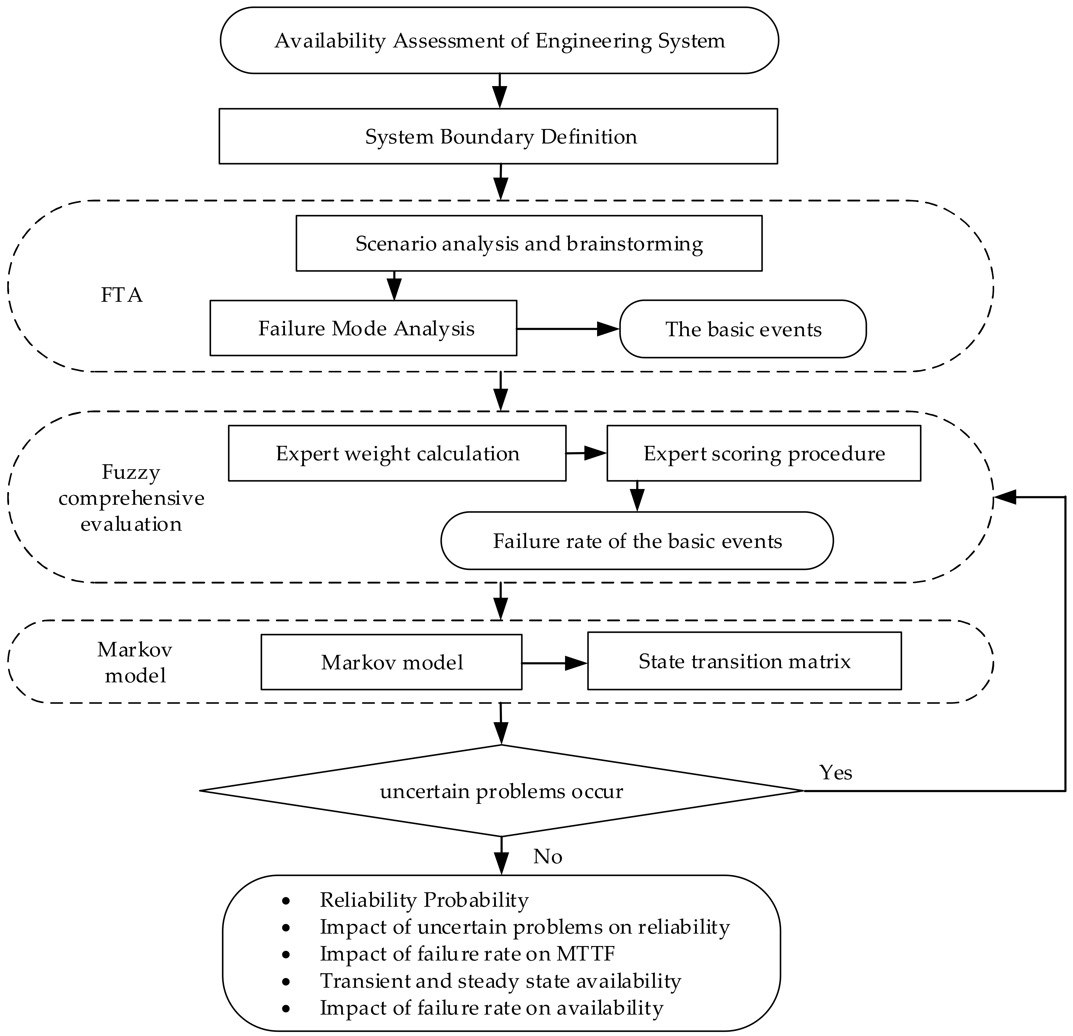
Aiming at the problems that the failure of engineering system is difficult to predict and the accurate statistics are lack, this paper presented the fuzzy Markov method integrating the fault tree analysis, fuzzy comprehensive evaluation and the Markov model. The method, comprehensively taking the normal operation, faults, maintenance, maintenance tests and periodic tests of the system into consideration, evaluate the availability, reliability index and the impact of uncertainty on system reliability. The proposed method was validated by the subsea wellhead connector.

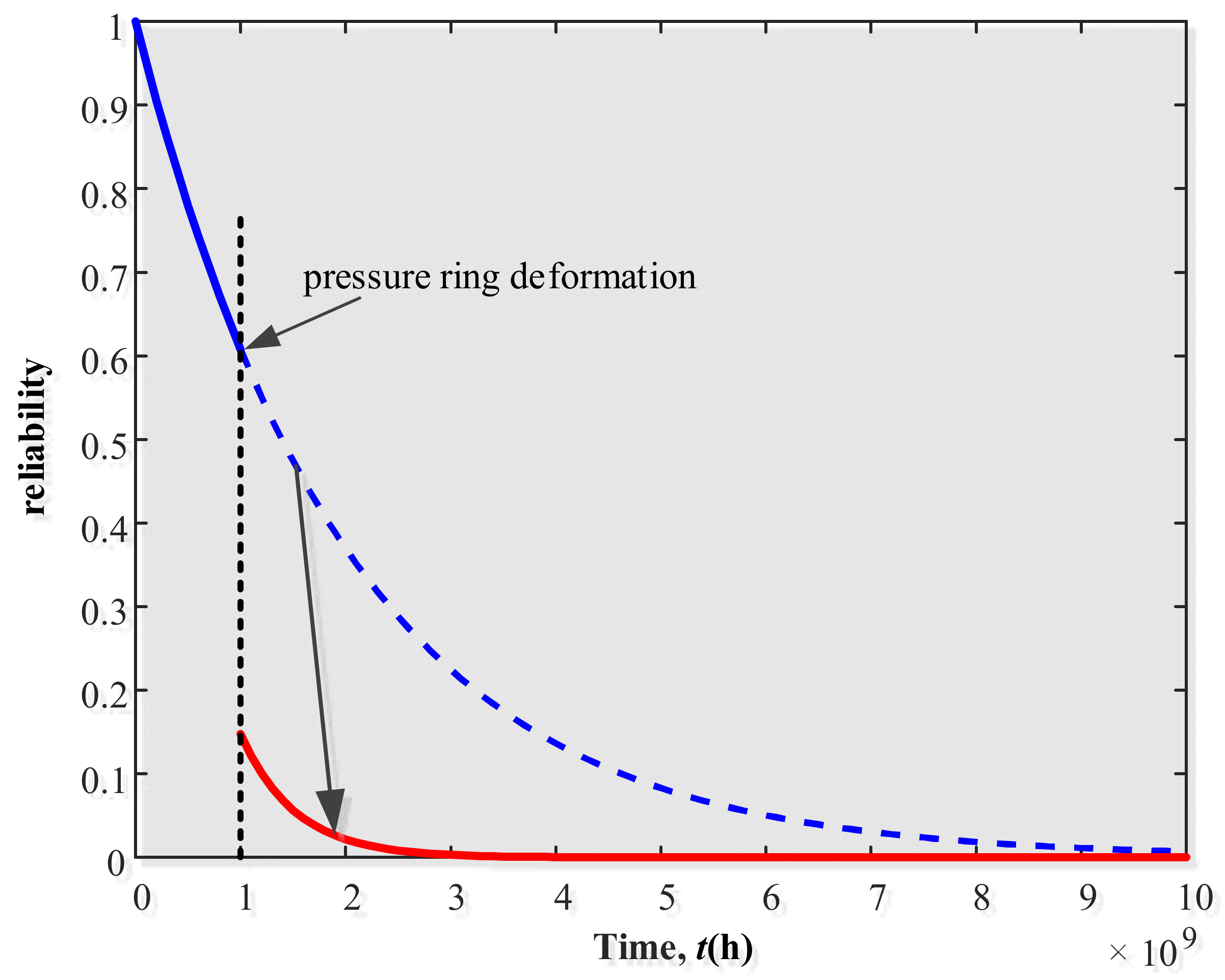
The results of the study of the subsea wellhead connector proved the benefits of the proposed methodology in general. Compared with other traditional methods, the fuzzy Markov can not only analyze risks, reliability, availability and maintainability, but also obtain unknown failure data. Moreover, the analysis of uncertainties was improved significantly. As shown in the discussion and results, the availability and reliability curves of the wellhead connector, the impacts of different components on system availability and the mean time to failure are obtained. According to the impact analysis, relevant recommendations for reliability design and relatively effective methods to improve system availability can be obtained. Most importantly, the model can update the system reliability according to the type of accident when the uncertainty occurs, which cannot be achieved by traditional methods. The analysis results obtained from this study can be provided as the reference for risk decision-making in the wellhead connector operations. The method in this paper can be used to obtain the corresponding conclusions of other complex engineering system.

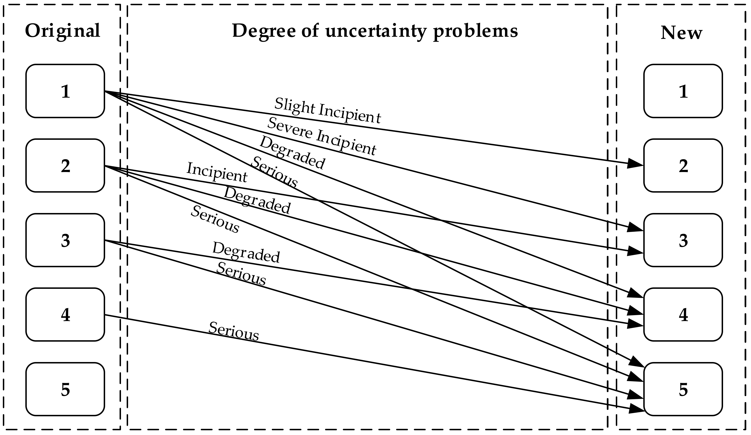
The fuzzy Markov proposed in this paper takes full advantage of the fault tree, fuzzy comprehensive evaluation and Markov method to make the analysis of risk, reliability, availability and uncertainty all in one, which a single traditional method cannot do. Compared with the previous fuzzy Markov method, the method adds dynamic iteration when failure of engineering systems occurs. It can follow the system state in real time, not limited to a fixed fuzzy range and any sets of cases, and can classify the uncertainties of different failure modes in different states of the system. According to the occurrence and severity of the uncertain problems, it can iterate the “Failure Cause Probability” of the corresponding failure mode, and update the real-time risk and reliability prediction model, which is more convenient and accurate for solving the uncertain problems of the engineering systems.

This paper assumes that the maintenance rate is constant. A future scope of the work can be directed toward the evaluation of the maintenance rate of engineering system, and more specific results can be obtained by referring to the method in this paper with specific maintenance rates.

References

1. Zhang, X.; Duan, M.; Mao, D.; Yu, Y.; Yu, J.; Wang, Y. A mathematical model of virtual simulation for deepwater installation of subsea production facilities. Ships Offshore Struct. 2017, 12, 182–195. [Google Scholar] [CrossRef]
2. Markowski, A.S.; Mannan, M.S.; Bigoszewska, A. Fuzzy logic for process safety analysis. J. Loss Prev. Process. Ind. 2009, 22, 695–702. [Google Scholar] [CrossRef]
3. Jozwiak, I.; Marianski, A.; Cwik, M. The probability of dying in a plane crash or having a safe flight. Aviation 2015, 19, 1–6. [Google Scholar] [CrossRef] [Green Version]
4. Markowski, A.S.; Mannan, M.S. Fuzzy logic for piping risk assessment (pfLOPA). J. Loss Prev. Process. Ind. 2009, 22, 921–927. [Google Scholar] [CrossRef]
5. Markowski, A.S.; Mannan, M.S. Fuzzy risk matrix. J. Hazard. Mater. 2008, 159, 152–157. [Google Scholar] [CrossRef]
6. Mentes, A.; Helvacioglu, I.H. An application of fuzzy fault tree analysis for spread mooring systems. Ocean. Eng. 2011, 38, 285–294. [Google Scholar] [CrossRef]
7. Babaleye, A.O.; Kurt, R.E.; Khan, F. Safety analysis of plugging and abandonment of oil and gas wells in uncertain conditions with limited data. Reliab. Eng. Syst. Saf. 2019, 188, 133–141. [Google Scholar] [CrossRef] [Green Version]
8. Yang, Z.L.; Bonsall, S.; Wall, A.; Wang, J.; Usman, M. A modified CREAM to human reliability quantification in marine engineering. Ocean. Eng. 2013, 58, 293–303. [Google Scholar] [CrossRef]
9. Lavasani, S.M.; Ramzali, N.; Sabzalipour, F.; Akyuz, E. Utilisation of Fuzzy Fault Tree Analysis (FFTA) for quantified risk analysis of leakage in abandoned oil and natural-gas wells. Ocean. Eng. 2015, 108, 729–737. [Google Scholar] [CrossRef]
10. Zhang, K.; Duan, M.; Luo, X.; Hou, G. A fuzzy risk matrix method and its application to the installation operation of subsea collet connector. J. Loss Prev. Process. Ind. 2017, 45, 147–159. [Google Scholar] [CrossRef]
11. Chang, Y.; Zhang, C.; Wu, X.; Shi, J.; Chen, G.; Ye, J.; Xu, L.; Xue, A. A Bayesian Network model for risk analysis of deepwater drilling riser fracture failure. Ocean. Eng. 2019, 181, 1–12. [Google Scholar] [CrossRef]
12. Zarei, E.; Khakzad, N.; Cozzani, V.; Reniers, G. Safety analysis of process systems using Fuzzy Bayesian Network (FBN). J. Loss Prev. Process. Ind. 2019, 57, 7–16. [Google Scholar] [CrossRef]
13. Yazdi, M.; Nedjati, A.; Abbassi, R. Fuzzy dynamic risk-based maintenance investment optimization for offshore process facilities. J. Loss Prev. Process. Ind. 2019, 57, 194–207. [Google Scholar] [CrossRef]
14. Soro, I.W.; Nourelfath, M.; Aït-Kadi, D. Performance evaluation of multi-state degraded systems with minimal repairs and imperfect preventive maintenance. Reliab. Eng. Syst. Saf. 2010, 95, 65–69. [Google Scholar] [CrossRef]
15. Kim, S.; Chung, S.; Yang, Y. Availability analysis of subsea blowout preventer using Markov model considering demand rate. Int. J. Nav. Archit. Ocean. Eng. 2014, 6, 775–787. [Google Scholar] [CrossRef] [Green Version]
16. Liu, Z.; Liu, Y.; Cai, B. Reliability analysis of the electrical control system of subsea blowout preventers using Markov models. PLoS ONE 2014, 9. [Google Scholar] [CrossRef]
17. Wang, X.; Jia, P.; Lizhang, H.; Wang, L.; Yun, F.; Wang, H. Reliability and Safety Modelling of the Electrical Control System of the Subsea Control Module Based on Markov and Multiple Beta Factor Model. IEEE Access 2019, 7, 6194–6208. [Google Scholar] [CrossRef]
18. Wang, L.; Wang, X.; Lizhang, H.; Jia, P.; Yun, F.; Wang, H. Design and reliability analysis of the electrical control system of the subsea control module. Proc. Inst. Mech. Eng. Part. I J. Syst. Control. Eng. 2019, 233, 720–733. [Google Scholar] [CrossRef]
19. Rahimi, T.; Jahan, H.K.; Blaabjerg, F.; Bahman, A.S.; Hosseini, S.H. Fuzzy-logic-based Mean Time to Failure (MTTF) analysis of interleaved dc-dc converters equipped with redundant-switch configuration. Appl. Sci. 2018, 9, 88. [Google Scholar] [CrossRef] [Green Version]
20. Shafiee, M.; Enjema, E.; Kolios, A. An integrated FTA-FMEA model for risk analysis of engineering systems: A case study of subsea blowout preventers. Appl. Sci. 2019, 9, 1192. [Google Scholar] [CrossRef] [Green Version]
21. Hong, C.; Estefen, S.F.; Wang, Y.; Lourenço, M.I. An integrated optimization model for the layout design of a subsea production system. Appl. Ocean. Res. 2018, 77, 1–13. [Google Scholar] [CrossRef]
22. Arnone, E.; Dialynas, Y.G.; Noto, L.V.; Bras, R.L. Parameter Uncertainty in Shallow Rainfall-triggered Landslide Modeling at Basin Scale: A Probabilistic Approach. Procedia Earth Planet. Sci. 2014, 9, 101–111. [Google Scholar] [CrossRef] [Green Version]
23. Aven, T.; Pedersen, L.M. On how to understand and present the uncertainties in production assurance analyses, with a case study related to a subsea production system. Reliab. Eng. Syst. Saf. 2014, 124, 165–170. [Google Scholar] [CrossRef]
24. Liu, Z.; Guo, T.; Chai, S. Probabilistic fatigue life prediction of bridge cables based on multiscaling and mesoscopic fracture mechanics. Appl. Sci. 2016, 6, 99. [Google Scholar] [CrossRef] [Green Version]
25. Gharehbaghi, K.; McManus, K.; Robson, K.; Eves, C.; Myers, M. Fuzzy Markov development for buried transportation bridges: Review of analysis and modeling technique. Int. J. Struct. Integr. 2020, 11. [Google Scholar] [CrossRef]
26. Song, X.; Man, J.; Fu, Z.; Wang, M.; Lu, J. Memory-based State Estimation of T–S Fuzzy Markov Jump Delayed Neural Networks with Reaction-Diffusion Terms. Neural Process. Lett. 2019, 50. [Google Scholar] [CrossRef]
27. Kavikumar, R.; Sakthivel, R.; Kwon, O.M.; Kaviarasan, B. Reliable non-fragile memory state feedback controller design for fuzzy Markov jump systems. Nonlinear Anal. Hybrid. Syst. 2020, 35. [Google Scholar] [CrossRef]
28. Guan, H.; Jie, H.; Guan, S.; Zhao, A. A novel fuzzy-Markov forecasting model for stock fluctuation time series. Evol. Intell. 2020, 13. [Google Scholar] [CrossRef]
29. Zhu, D.M.; Ching, W.K.; Guu, S.M. Sufficient conditions for the ergodicity of fuzzy Markov chains. Fuzzy Sets Syst. 2016, 304. [Google Scholar] [CrossRef]
30. Austin, A.M.; Douglass, M.J.J.; Nguyen, G.T.; Penfold, S.N. Patient selection for proton therapy: A radiobiological fuzzy Markov model incorporating robust plan analysis. Phys. Eng. Sci. Med. 2020, 43. [Google Scholar] [CrossRef]
31. Fathi-Vajargah, B.; Gharehdaghi, M. Improvement of fuzzy image contrast enhancement using simulated ergodic fuzzy Markov chains. Math. Probl. Eng. 2014, 2014. [Google Scholar] [CrossRef]
32. Pathan, M.I.; Al-Muhaini, M. Data Forecasting and Storage Sizing for PV Battery System Using Fuzzy Markov Chain Model. Arab. J. Sci. Eng. 2020, 45. [Google Scholar] [CrossRef]
33. Li, J. Fault-Event Trees Based Probabilistic Safety Analysis of a Boiling Water Nuclear Reactor’s Core Meltdown and Minor Damage Frequencies. Safety 2020, 6, 28. [Google Scholar] [CrossRef]
34. Khakzad, N.; Khan, F.; Amyotte, P. Dynamic risk analysis using bow-tie approach. Reliab. Eng. Syst. Saf. 2012, 104, 36–44. [Google Scholar] [CrossRef]
35. Lavasani, S.M.M.; Wang, J.; Yang, Z.; Finlay, J. Application of MADM in a fuzzy environment for selecting the best barrier for offshore wells. Expert Syst. Appl. 2012, 39, 2466–2478. [Google Scholar] [CrossRef]
36. Mahmood, Y.A.; Ahmadi, A.; Verma, A.K.; Srividya, A.; Kumar, U. Fuzzy fault tree analysis: A review of concept and application. Int. J. Syst. Assur. Eng. Manag. 2013, 4, 19–32. [Google Scholar] [CrossRef]
37. Lin, C.T.; Wang, M.J.J. Hybrid fault tree analysis using fuzzy sets. Reliab. Eng. Syst. Saf. 1997, 58, 205–213. [Google Scholar] [CrossRef]
38. Onisawa, T. An approach to human reliability in man-machine systems using error possibility. Fuzzy Sets Syst. 1988, 27, 87–103. [Google Scholar] [CrossRef]
39. Veritas, D.N. Offshore Reliability Data Handbook, 4th ed.; OREDA: Høvik, Norway, 2002. [Google Scholar]
40. Holand, P.; Awan, H. Reliability of Deepwater Subsea BOP Systems and Well Kicks. Methodology 2012, 08, 39–42. [Google Scholar]
41. Veeramany, A.; Pandey, M.D. Reliability analysis of nuclear component cooling water system using semi-Markov process model. Nucl. Eng. Des. 2011, 241, 1799–1806. [Google Scholar] [CrossRef]
42. Borcsok, J.; Ugljesa, E.; Machmur, D. Calculation of MTTF values with Markov Models for Safety Instrumented Systems. In Proceedings of the 7th WSEAS International Conference on APPLIED COMPUTER SCIENCE, Venice, Italy, 21–23 November 2007; pp. 30–35. [Google Scholar]
43. Khakzad, N.; Khan, F.; Amyotte, P. Safety analysis in process facilities: Comparison of fault tree and Bayesian network approaches. Reliab. Eng. Syst. Saf. 2011, 96, 925–932. [Google Scholar] [CrossRef]
44. Bobbio, A.; Portinale, L.; Minichino, M.; Ciancamerla, E. Improving the Analysis of Dependable Systems by Mapping Fault Trees into Bayesian Networks. Realiability Eng. Syst. Saf. 2001, 71, 249–260. [Google Scholar] [CrossRef]
45. Hänninen, M. Bayesian networks for maritime traffic accident prevention: Benefits and challenges. Accid. Anal. Prev. 2014, 73, 305–312. [Google Scholar] [CrossRef] [PubMed]
46. Zhang, H.; Innal, F.; Dufour, F.; Dutuit, Y. Piecewise Deterministic Markov Processes based approach applied to an offshore oil production system. Reliab. Eng. Syst. Saf. 2014, 126, 126–134. [Google Scholar] [CrossRef]
Figure 1. Fuzzy Markov integration framework. FTA: Fault Tree Analysis; MTTF: Mean time to failure.
Applsci 10 06902 g001
Figure 2. “Failure Cause Probability” change method.
Applsci 10 06902 g002
Figure 3. A framework of fuzzy comprehensive evaluation method.
Applsci 10 06902 g003
Figure 4. Expert scoring risk matrix. Very Low (VL), Low (L), Fairly Low (FL), Medium (M), Fairly High (FH), High (H) and Very High (VH).
Applsci 10 06902 g004
Figure 5. Diagram of fuzzy membership functions. Very Low (VL), Low (L), Fairly Low (FL), Medium (M), Fairly High (FH), High (H) and Very High (VH).
Applsci 10 06902 g005
Figure 6. The composition of the wellhead connector.
Applsci 10 06902 g006
Figure 7. Fault tree analysis model of wellhead connector.
Applsci 10 06902 g007
Figure 8. Markov transition diagram of subsea wellhead connector.
Applsci 10 06902 g008
Figure 9. Reliability and transient availability of subsea wellhead connector.
Applsci 10 06902 g009
Figure 10. Reliability of subsea wellhead connector when pressure ring deformation occurs at t = 109 h.
Applsci 10 06902 g010
Figure 11. Impacts of transfer rates λ118 (a), λ19 (b), λ20 and λ24 (c), λ21 and λ23 (d) and λ22 (e) on stable availability.
Applsci 10 06902 g011
Figure 12. Impacts of transition rates λ1–λ18 (a), λ21 and λ22 (b) and λ24 (c) on MTTF.
Applsci 10 06902 g012