Smart Grid for Industry Using Multi-Agent Reinforcement Learning

 and
and
Abstract
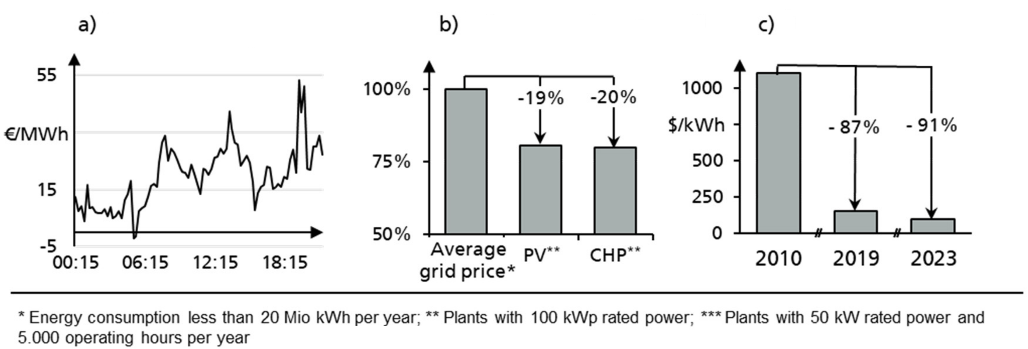
1. Introduction
2. Fundamentals
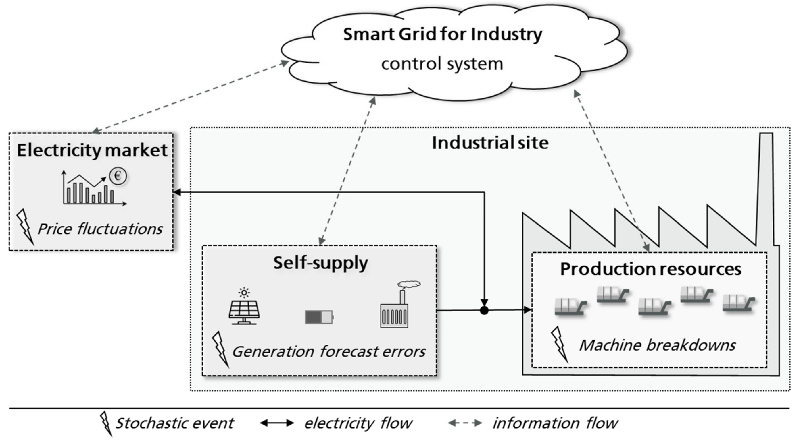
2.1. Industrial Electricity Supply
- Power procurement [19,20]: In this case, the manufacturing companies buy the required amount of electricity from external sources. The general billing interval of the entire electricity market is 15 min. There are two main options for procurement:
- ○
- Utility company: Industrial companies may directly rely on power utility companies, which in general provide constant prices, thus completely bearing the price risks.
- ○
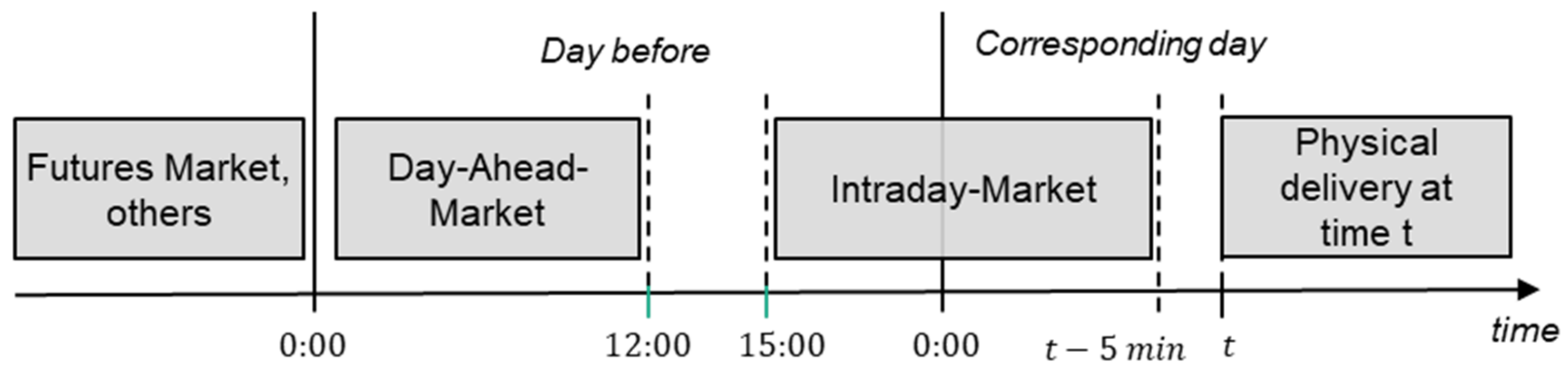
- Market trading: Companies can actively take part in the electricity market, either trading directly or relying on a suitable aggregator. There are several electricity markets which can be characterized by their lead time. It is worth noting that there is always some lead time between order purchasing and the actual delivery and consumption of the electricity (see Figure 3). The shortest lead time is offered by the intraday market, in which electricity can be bought at least 5 min before delivery. In case a company has bought electricity within a specified interval, it must ensure that the power is actually consumed. In general, a tolerance bandwidth of ±5 to 10% is granted. Otherwise, there is a risk of receiving high penalties.
- Self-supply [21,22]: Manufacturing companies may dispose of their own power generation facilities, which enable them to generate their electricity on-site. Depending on the relevant control characteristics, power plants can be divided into two groups:
- ○
- Variable power sources (VPS): The power generation of these sources is difficult to control because it is highly dependent on the current weather conditions. The only control option is to cut off their power. However, since VPS do not entail any working expenses, this is not recommended. The most important kinds of VPS are solar and wind power plants.
- ○
- Controllable power sources (CPS): The power output of CPS can be controlled and adapted within a specified range. In the manufacturing field, combined heat and power plants (CHP) are widely used and are assigned to this category.
- Battery systems: Batteries consist of electrochemical, rechargeable cells and are very suitable for storing electricity for several hours or days [23]. However, the cells suffer from degradation over time. The extent of the degradation strongly depends on the charging cycles the battery is exposed to [24]. As a result, there exist several modelling approaches for considering the degradation process within a battery control strategy [25].
2.2. Approaches for Production Control
- ○
- Reactive control strategy: The jobs are reactively scheduled based on simply dispatching rules like first-in-first-out (FIFO) or earliest-deadline-first (EDF). After finishing a job, the next job is selected, so no fixed production schedule is determined. In doing so, decisions can be made very quickly, whereas the solution quality is limited.
- ○
- Predictive-reactive control strategy: A deterministic schedule is calculated for a specified production period so as to optimize the given objectives. However, every stochastic event during the production period requires a schedule update, which makes this approach computationally expensive.
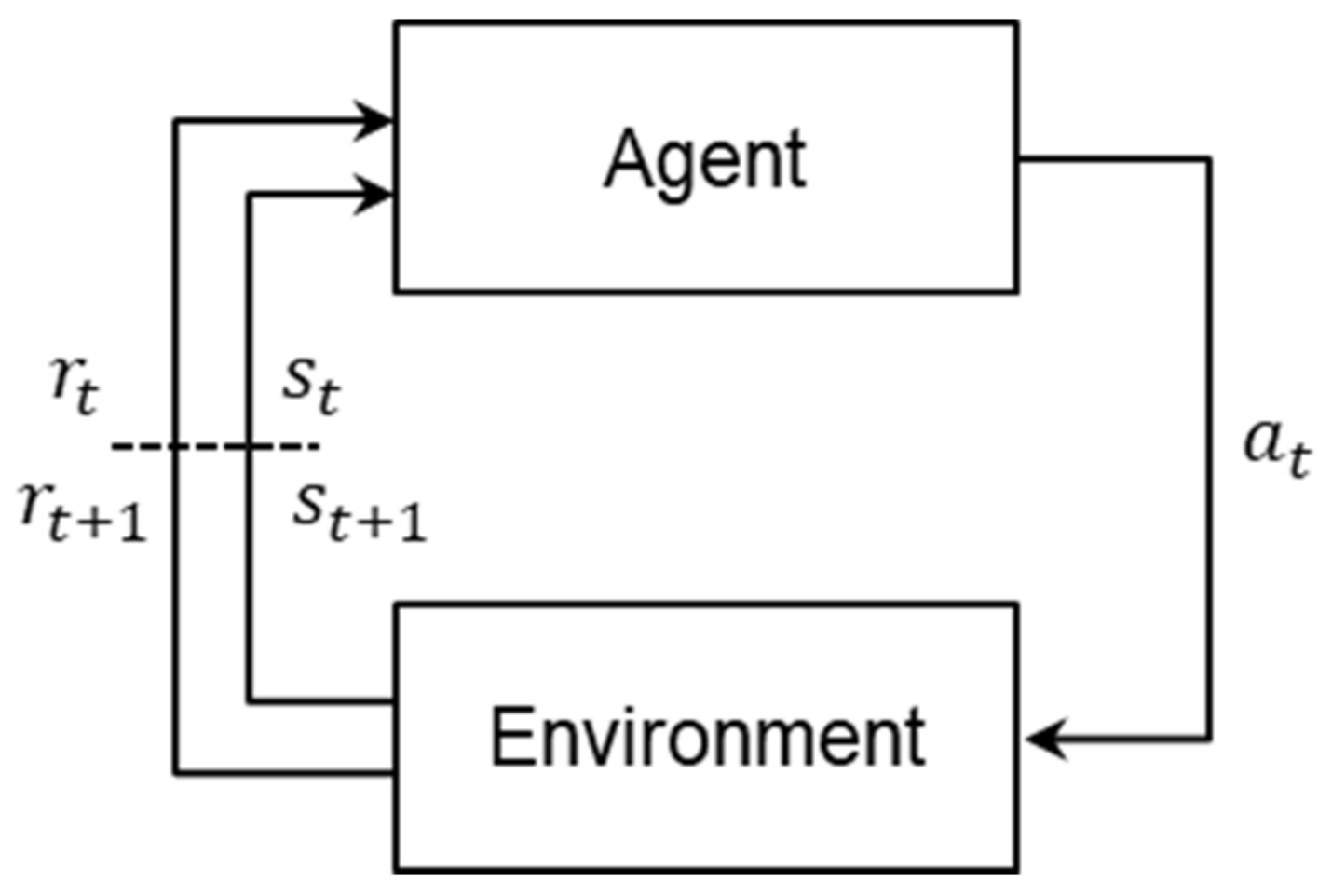
2.3. Multi-Agent Reinforcement Learning
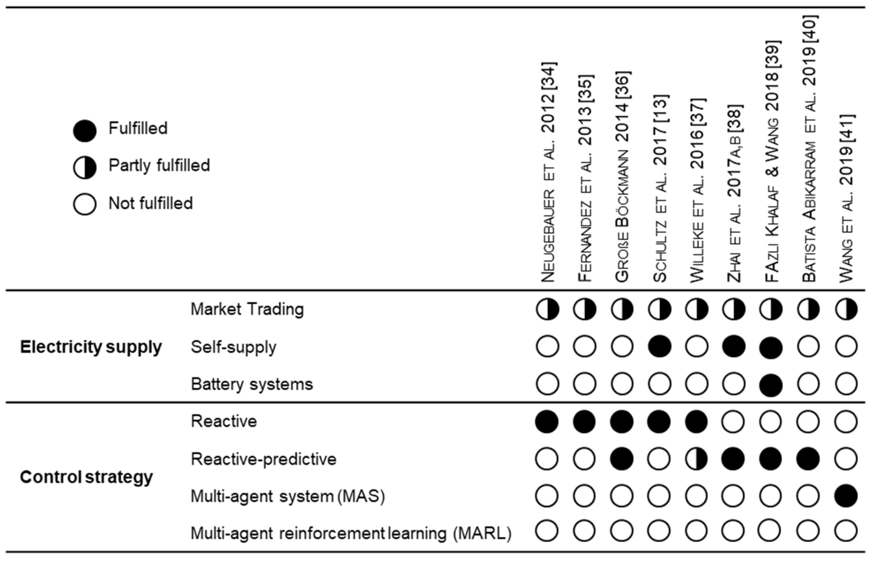
3. Literature Review
4. Proposed MARL Approach
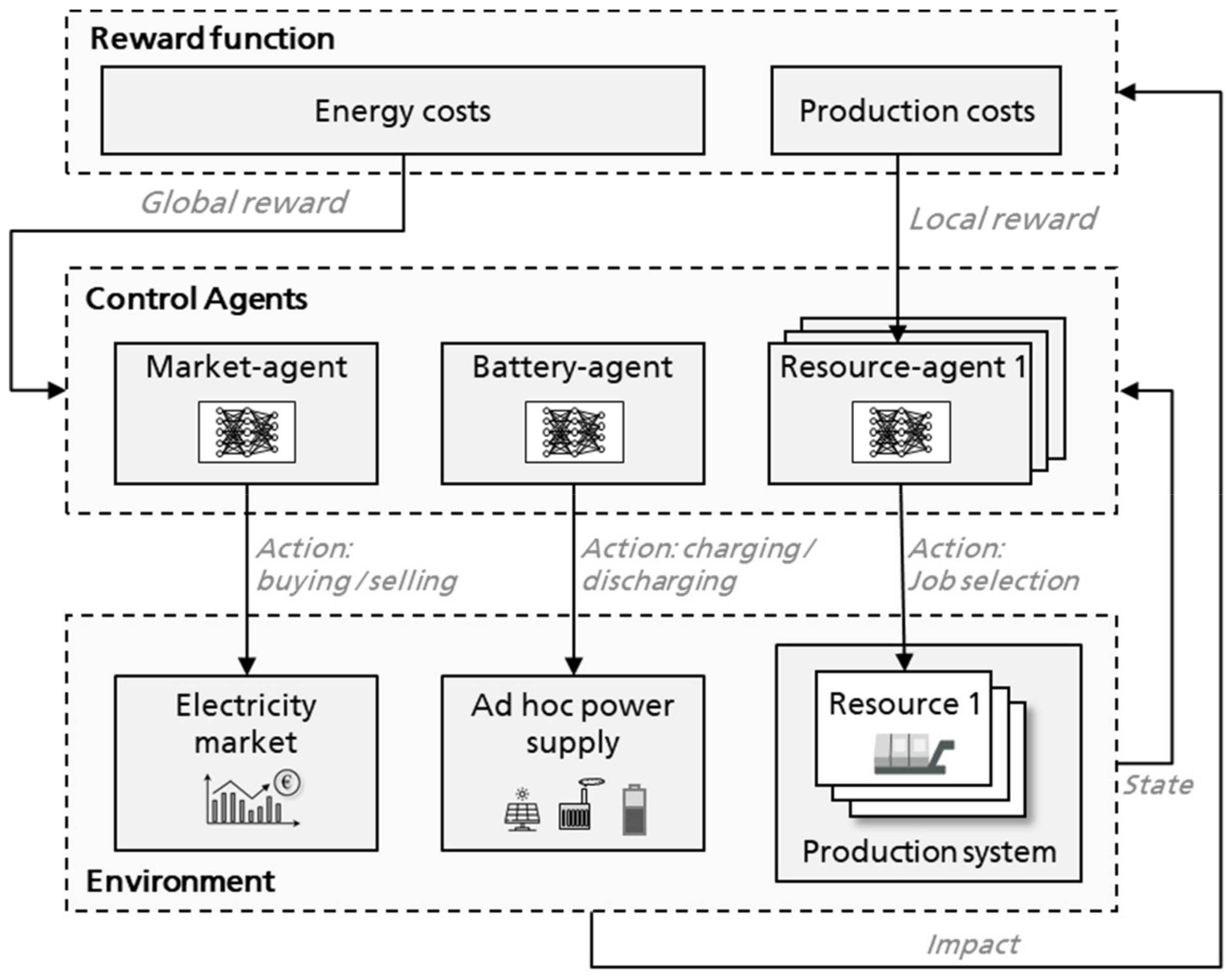
4.1. System Overview
4.2. Environment
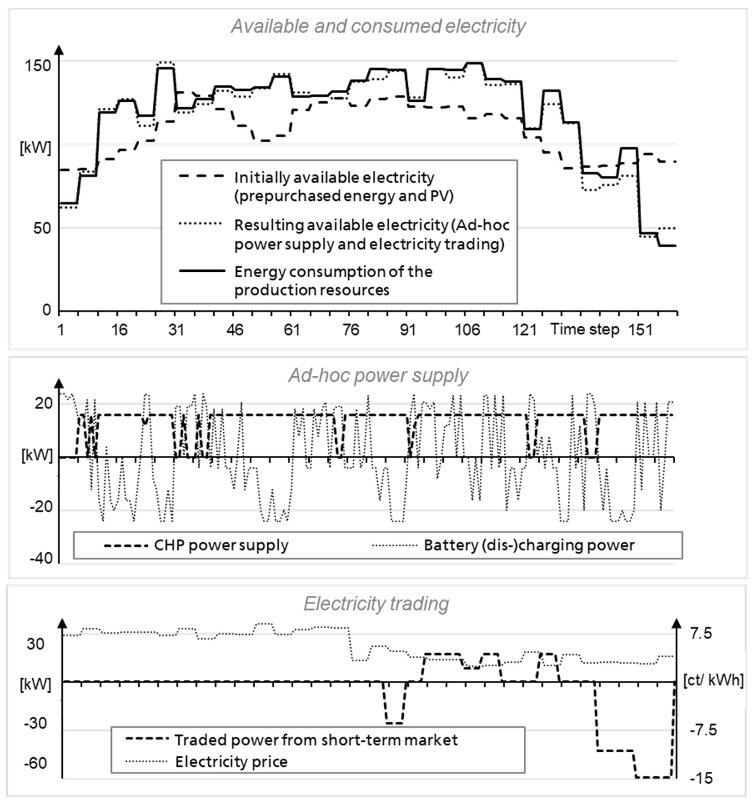
4.2.1. Electricity Market
4.2.2. Ad-hoc Power Supply
- ○
- The electricity bought from the intraday market and other prior purchased power should always be consumed in order to avoid penalty costs.
- ○
- Power from VPS should also be consumed since this does not result in any costs. Only in the case of excessively low power demand from the production system can VPS be temporarily cut off so as to avoid penalty costs for consuming less electricity than previously purchased.
- ○
- The remaining power demand which cannot be met by VPS and the electricity purchased from the market has to be provided by the battery and the CPS.
- ○
- Compensating for a deficit of power availability and demand with energy from the public grid should be avoided, as this can incur high costs.
- Calculation of the charging/discharging power of the battery system based on RL (Battery Agent), whereas the total state of all elements in the power supply (battery, VPS, CPS, prior purchased power) and the current demand from production side is considered.
- The gap between expected power consumption and available power from VPS, battery power as well as purchased electricity from the markets is settled by CPS as much as possible.
- If there is more energy available than the expected demand, cut-off power generation of VPS to balance demand and supply as much as possible.
- The remaining deficit is settled by the public grid.
4.2.3. Production System
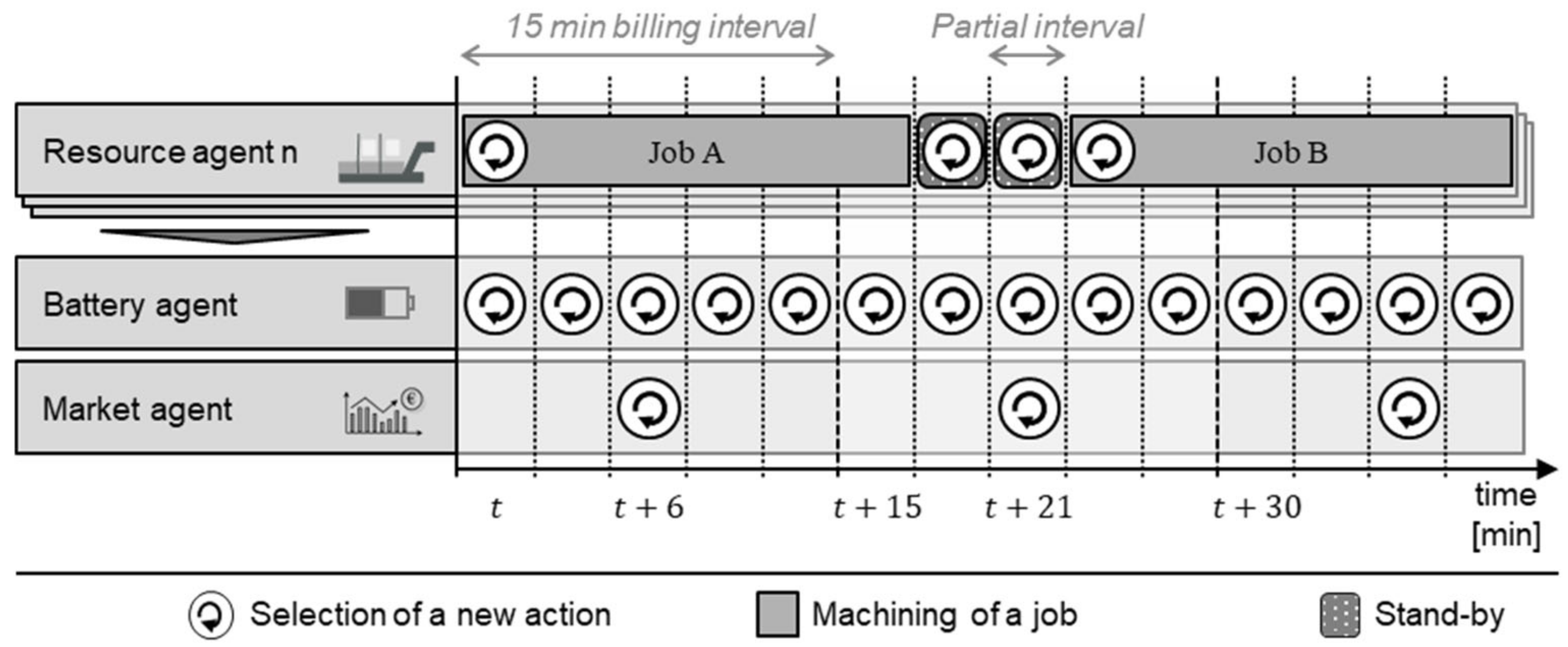
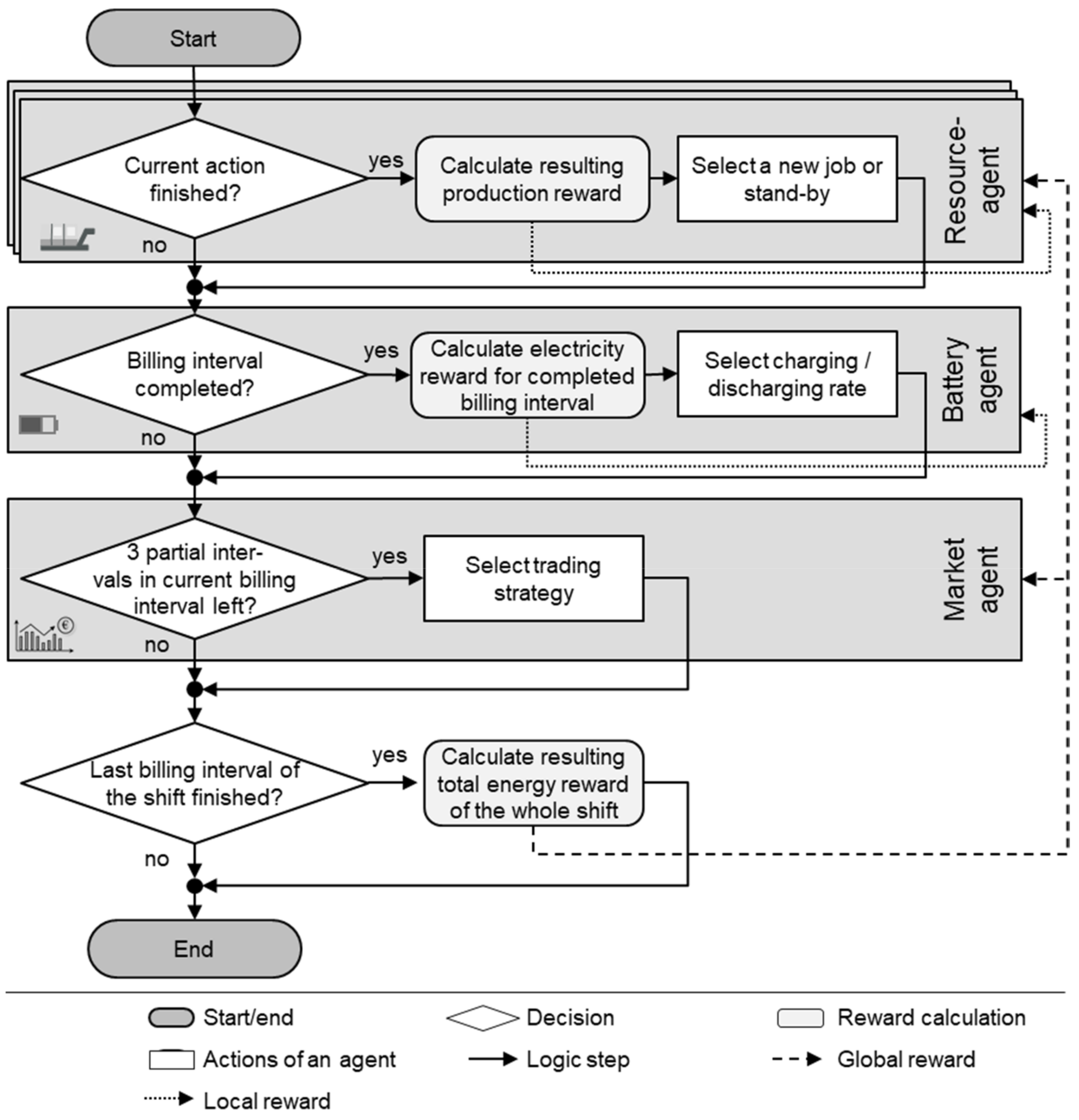
4.2.4. System Sequence
4.3. State and Action Space
4.4. Reward Calculation and Assignment
4.5. Training Procedure
5. Case Study
5.1. Set-Up
5.2. Validation Scenarios
- ○
- Reactive control strategy (RCS): The reactive production control was based on the commonly used dispatching rule EDF. A widespread rule-based heuristic was developed to control the battery and CHP [49]. In this case, the battery power was adjusted, with the goal of maximizing CHP power generation and minimizing the resulting deviation between power demand and supply as much as possible. The generation of VPS was only cut off when there was still excessive power available while the battery was on maximum charging power and the CHP completely turned off. Since market trading is not possible using a rule-based method, there was no electricity trading in this scenario.
- ○
- Predictive-reactive control strategy (PCS): An optimization approach based on the metaheuristic Simulated Annealing was applied to control the overall system. The production plan was rescheduled both in the beginning of an episode and every time that a stochastic event occurred. The state transitions were thereby selected in an arbitrary manner, either by changing the starting time or the sequence of jobs, trading electricity, or adjusting the battery power. The implementation was based on [50]; for the parameters of starting temperature, minimum temperature, alpha, and iterations, values of 10, 0.01, 0.9999, and 100 were chosen.
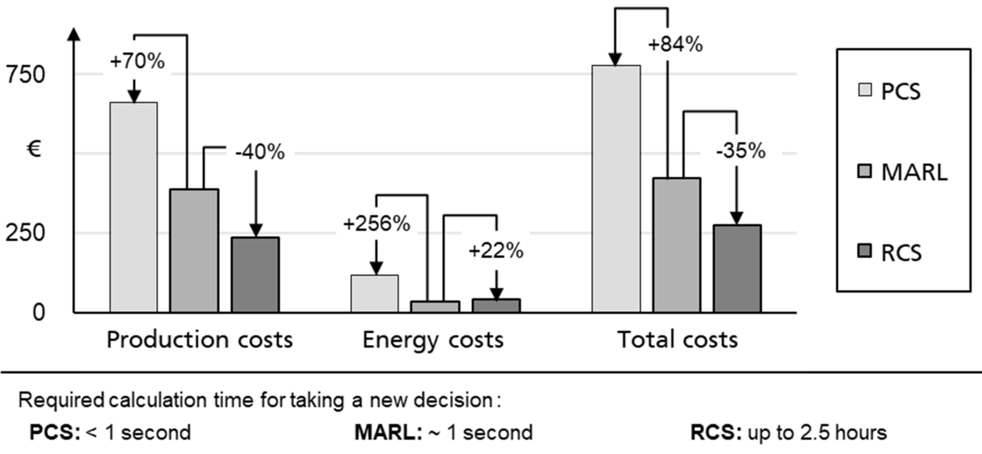
5.3. Results and Discussion
6. Conclusions
Author Contributions
Funding
Conflicts of Interest
References
- Prognos, A.G.; Wünsch, M.; Fraunhofer, I.F.A.M.; Eikmeier, B.; Gailfuß, M. Potenzial-und Kosten-Nutzen-Analyse zu den Einsatzmöglichkeiten von Kraft-Wärme-Kopplung (Umsetzung der EU-Energieeffizienzrichtlinie) sowie Evaluierung des KWKG im Jahr 2014; Endbericht zum Projekt IC: Berlin, Germany, 2014. [Google Scholar]
- BDEW. Strompreisanalyse Mai 2018: Haushalte und Industrie. Bundesverband der Energie-und Wasserwirtschaft e.V; BDEW Bundesverband der Energie- und Wasserwirtschaft e.V.: Berlin, Germany, 2018. [Google Scholar]
- Reinhart, G.; Reinhardt, S.; Graßl, M. Energieflexible Produktionssysteme. Ein-führungen zur Bewertung der Energieeffizienz von Produktionssystemen. Werkstattstechnik Online 2012, 102, 622–628. [Google Scholar]
- Knupfer, S.M.; Hensley, R.; Hertzke, P.; Schaufuss, P.; Laverty, N.; Kramer, N. Electrifiying Insights: How Automakers can Drive Electrified Vehicle Sales and Profitability; McKinsey&Company: Detroit, MI, USA , 2017. [Google Scholar]
- Stolle, T.; Hankeln, C.; Blaurock, J. Die Bedeutung der Energiespeicherbranche für das Energiesystem und die Gesamtwirtschaft in Deutschland. Energiewirtsch. Tagesfragen. 2018, 9, 54–56. [Google Scholar]
- EPEX Spot. Market Data. 2020. Available online: https://www.epexspot.com/en/market-data (accessed on 6 May 2020).
- Kost, C.; Shammugam, S.; Jülich, V.; Nguyen, H.T.; Schlegl, T. Stromgestehungskosten Erneuerbare Energien. Fraunhofer ISE: Freiburg, Germany, 2018. [Google Scholar]
- Wünsch, M.; Eikmeier, B.; Eberhard, J.; Gailfuß, M. Potenzial-und Kosten-Nutzen-Analyse zu den Einsatzmöglichkeiten von Kraft-Wärme-Kopplung (Umsetzung der EU-Energieeffizienzrichtlinie) sowie Evaluierung des KWKG im Jahr 2014. 2014. Available online: https://ec.europa.eu/energy/sites/ener/files/documents/151221%20Mitteilung%20an%20KOM%20EED%20KWK%20Anlage%20Analyse.pdf (accessed on 20 May 2020).
- Beier, J. Simulation Approach Towards Energy Flexible Manufacturing Systems; Springer International Publishing: Cham, Switzerland, 2017; p. 22796. [Google Scholar]
- Fang, X.; Misra, S.; Xue, G.; Yang, D. Smart grid—The new and improved power grid: A survey. IEEE Commun. Surv. Tutor. 2012, 14, 944–980. [Google Scholar] [CrossRef]
- Lödding, H. Handbook of Manufacturing Control: Fundamentals, Description, Configuration; Springer: Berlin/Heidelberg, Germany, 2013. [Google Scholar]
- Schultz, C.; Bayer, C.; Roesch, M.; Braunreuther, S.; Reinhart, G. Integration of an automated load management in a manufacturing execution system. In Proceedings of the 2017 IEEE International Conference on Industrial Engineering and Engineering Management (IEEM), Singapore, 10–13 December 2017; IEEE: Piscataway, NJ, USA, 2017; pp. 494–498. [Google Scholar]
- Gabel, T. Multi-Agent Reinforcement Learning Approaches for Distributed Job-Shop Scheduling Problems. Ph.D. Thesis, University of Osnabrück, Osnabrück, Germany, 2009. [Google Scholar]
- Kuhnle, A.; Schäfer, L.; Stricker, N.; Lanza, G. Design, implementation and evaluation of reinforcement learning for an adaptive order dispatching in job shop manufacturing systems. Procedia CIRP 2019, 81, 234–239. [Google Scholar] [CrossRef]
- Wang, Y.; Liu, H.; Zheng, W.; Xia, Y.; Li, Y.; Chen, P.; Guo, K.; Xie, H. Multi-objective workflow scheduling with Deep-Q-network-based multi-agent reinforcement learning. IEEE Access 2019, 7, 39974–39982. [Google Scholar] [CrossRef]
- Waschneck, B.; Reichstaller, A.; Belzner, L.; Altenmuller, T.; Bauernhansl, T.; Knapp, A.; Kyek, A. Deep reinforcement learning for semiconductor production scheduling. In Proceedings of the 29th Annual SEMI Advanced Semiconductor Manufacturing Conference 2018 (ASMC 2018), Saratoga Springs, NY, USA, 30 April–3 May 2018; Institute of Electrical and Electronics Engineers: Piscataway, NJ, USA, 2018; pp. 301–306. [Google Scholar]
- Jiang, B.; Fei, Y. Smart home in smart microgrid: A cost-effective energy ecosystem with intelligent hierarchical agents. IEEE Trans. Smart Grid 2015, 6, 3–13. [Google Scholar] [CrossRef]
- Mbuwir, B.V.; Kaffash, M.; Deconinck, G. Battery scheduling in a residential multi-carrier energy system using reinforcement learning. In Proceedings of the 2018 IEEE International Conference on Communications, Control, and Computing Technologies for Smart Grids (SmartGridComm), Aalborg, Denmark, 29–31 October 2018; IEEE: Piscataway, NJ, USA, 2018; pp. 1–6. [Google Scholar]
- Berg, M.; Borchert, S. Strategischer Energieeinkauf: Der Energieeinkauf Zwischen Liberalisierten Märkten und Einer Wechselhaften Energiepolitik in Deutschland; BME: Frankfurt am Main, Germany, 2014. [Google Scholar]
- Bertsch, J.; Fridgen, G.; Sachs, T.; Schöpf, M.; Schweter, H.; Sitzmann, A. Ausgangsbedingungen für die Vermarktung von Nachfrageflexibilität: Status-Quo-Analyse und Metastudie; Bayreuther Arbeitspapiere zur Wirtschaftsinformatik 66: Bayreuth, Germany, 2017. [Google Scholar]
- Günther, M. Energieeffizienz durch erneuerbare Energien: Möglichkeiten, Potenziale, Systeme; Springer: Vieweg, Wiesbaden, 2015; p. 193. [Google Scholar]
- Keller, F.; Braunreuther, S.; Reinhart, G. Integration of on-site energy generation into production planning systems. Procedia CIRP 2016, 48, 254–258. [Google Scholar] [CrossRef]
- Köhler, A.; Baron, Y.; Bulach, W.; Heinemann, C.; Vogel, M.; Behrendt, S.; Degel, M.; Krauß, N.; Buchert, M. Studie: Ökologische und ökonomische Bewertung des Ressourcenaufwands—Stationäre Energiespeichersysteme in der Industriellen Produktion; VDI ZRE: Berlin, Germany, 2018. [Google Scholar]
- Vetter, J.; Novak, P.; Wagner, M.; Veit, C.; Möller, K.C.; Besenhard, J.; Winter, M.; Wohlfahrt-Mehrens, M.; Vogler, C.; Hammouche, A. Ageing mechanisms in lithium-ion batteries. J. Power Sources 2005, 147, 269–281. [Google Scholar] [CrossRef]
- Safari, M.; Morcrette, M.; Teyssot, A.; Delacourt, C. Multimodal physics-based aging model for life prediction of li-ion batteries. J. Electrochem. Soc. 2009, 156, A145. [Google Scholar] [CrossRef]
- Ouelhadj, D.; Petrovic, S. A survey of dynamic scheduling in manufacturing systems. J. Sched. 2008, 12, 417–431. [Google Scholar] [CrossRef]
- Vieira, G.E.; Herrmann, J.W.; Lin, E. Rescheduling manufacturing systems: A framework of strategies, policies, and methods. J. Sched. 2003, 6, 39–62. [Google Scholar] [CrossRef]
- Shen, W.; Hao, Q.; Yoon, H.J.; Norrie, D.H. Applications of agent-based systems in intelligent manufacturing: An updated review. Adv. Eng. Inform. 2006, 20, 415–431. [Google Scholar] [CrossRef]
- Shen, W.; Norrie, D.H.; Barthès, J.P. Multi-Agent Systems for Concurrent Intelligent Design and Manufacturing; Taylor & Francis: London, UK, 2001; p. 386. [Google Scholar]
- Sutton, R.S.; Barto, A. Reinforcement Learning: An Introduction, 2nd ed.; The MIT Press: Cambridge, MA, USA, 2018; p. 526. [Google Scholar]
- Ngyen, D.T.; Kumar, A.; Lau, H.C. Credit assignment for collective multiagent RL with global rewards. In Proceedings of the 32nd International Conference on Neural Information Processing System NIPS’18, Montréal, QC, Canada, 2–8 December 2018; pp. 8113–8124. [Google Scholar]
- Silver, D.; Huang, A.; Maddison, C.J.; Guez, A.; Sifre, L.; Driessche, G.V.D.; Schrittwieser, J.; Antonoglou, I.; Panneershelvam, V.; Lanctot, M.; et al. Mastering the game of Go with deep neural networks and tree search. Nature 2016, 529, 484–489. [Google Scholar] [CrossRef]
- Neugebauer, R.; Putz, M.; Schlegel, A.; Langer, T.; Franz, E.; Lorenz, S. Energy-sensitive production control in mixed model manufacturing processes. In Leveraging Technology for A Sustainable World, Proceedings of the 19th CIRP Conference on Life Cycle Engineering, University of California at Berkeley, Berkeley, CA, USA, 23–25 May 2012; LCE 2012; Dornfeld, D.A., Linke, B.S., Eds.; Springer: Berlin/Heidelberg, Germany, 2012; pp. 399–404. [Google Scholar]
- Fernandez, M.; Li, L.; Sun, Z. “Just-for-Peak” buffer inventory for peak electricity demand reduction of manufacturing systems. Int. J. Prod. Econ. 2013, 146, 178–184. [Google Scholar] [CrossRef]
- Böckmann, M.G. Senkung der Produktionskosten durch Gestaltung eines Energieregelkreis-Konzeptes; Apprimus-Verlag: Aachen, Germany, 2014; p. 166. [Google Scholar]
- Willeke, S.; Ullmann, G.; Nyhuis, P. Method for an energy-cost-oriented manufacturing control to reduce energy costs: Energy cost reduction by using a new sequencing method. In Proceedings of the ICIMSA 2016 International Conference on Industrial Engineering, Management Science and Applications, Jeju Island, Korea, 23–26 May 2016; IEEE: Piscataway, NJ, USA, 2016; pp. 1–5. [Google Scholar]
- Zhai, Y.; Biel, K.; Zhao, F.; Sutherland, J. Dynamic scheduling of a flow shop with on-site wind generation for energy cost reduction under real time electricity pricing. CIRP Ann. 2017, 66, 41–44. [Google Scholar] [CrossRef]
- Khalaf, A.F.; Wang, Y. Energy-cost-aware flow shop scheduling considering intermittent renewables, energy storage, and real-time electricity pricing. Int. J. Energy Res. 2018, 42, 3928–3942. [Google Scholar] [CrossRef]
- Abikarram, J.B.; McConky, K.; Proano, R.A. Energy cost minimization for unrelated parallel machine scheduling under real time and demand charge pricing. J. Clean. Prod. 2019, 208, 232–242. [Google Scholar] [CrossRef]
- Wang, J.; Zhang, Y.; Liu, Y.; Wu, N. Multiagent and bargaining-game-based real-time scheduling for internet of things-enabled flexible job shop. IEEE Internet Things J. 2019, 6, 2518–2531. [Google Scholar] [CrossRef]
- Schaumann, G.; Schmitz, K.W. Kraft-Wärme-Kopplung, Vollständig Bearbeitete und Erweiterte, 4th ed.; Springer: Berlin/Heidelberg, Germany, 2010. [Google Scholar]
- Xu, B.; Oudalov, A.; Ulbig, A.; Andersson, G.; Kirschen, D.S. Modeling of lithium-ion battery degradation for cell life assessment. IEEE Trans. Smart Grid 2016, 9, 1131–1140. [Google Scholar] [CrossRef]
- Schultz, C.; Braun, S.; Braunreuther, S.; Reinhart, G. Integration of load management into an energy-oriented production control. Procedia Manuf. 2017, 8, 144–151. [Google Scholar] [CrossRef]
- Roesch, M.; Linder, C.; Bruckdorfer, C.; Hohmann, A.; Reinhart, G. Industrial Load Management using Multi-Agent Reinforcement Learning for Rescheduling. In Proceedings of the 2019 Second International Conference on Artificial Intelligence for Industries (AI4I) (IEEE), Laguna Hills, CA, USA, 25–27 September 2019; pp. 99–102. [Google Scholar]
- Roesch, M.; Berger, C.; Braunreuther, S.; Reinhart, G. Cost-Model for Energy-Oriented Production Control; IEEE: Piscataway, NJ, USA, 2018; pp. 158–162. [Google Scholar]
- Schulman, J.; Wolski, F.; Dhariwal, P.; Radford, A.; Klimov, O. Proximal policy optimization algorithms. arXiv 2017, arXiv:1707.06347. [Google Scholar]
- Schulman, J.; Moritz, P.; Levine, S.; Jordan, M.; Abbeel, P. High-dimensional continuous control using generalized advantage estimation. arXiv 2015, arXiv:1506.02438. [Google Scholar]
- Loon, K.W.; Graesser, L.; Cvitkovic, M. SLM Lab: A Comprehensive benchmark and modular software framework for reproducible deep reinforcement learning. arXiv 2019, arXiv:1912.12482. [Google Scholar]
- Weniger, J.; Bergner, J.; Tjaden, T.; Quaschning, V. Bedeutung von prognosebasierten Betriebsstrategien für die Netzintegration von PV-Speichersystemen. In Proceedings of the 29th Symposium Photovoltaische Solarenergie, Bad Staffelstein, Germany, 12–14 March 2014. [Google Scholar]
- Van Laarhoven, P.J.M.; Aarts, E.H.L. Simulated Annealing: Theory and Applications; Kluwer: Dordrecht, The Netherlands, 1992; p. 187. [Google Scholar]
- Liang, E.; Liaw, R.; Moritz, P.; Nishihara, R.; Fox, R.; Goldberg, K.; Gonzalez, J.E.; Jordan, M.I.; Stoica, I. RLlib: Abstractions for distributed reinforcement learning. arXiv 2017, arXiv:1712.09381. [Google Scholar]
- Badia, A.P.; Sprechmann, P.; Vitvitskyi, P.; Guo, D.; Piot, B.; Kapturowski, S.; Tieleman, O.; Arjovsky, M.; Pritzel, A.; Bolt, A.; et al. Never Give Up: Learning Directed Exploration Strategies, International Conference on Learning Representations. arXiv 2020, arXiv:2002.06038. [Google Scholar]


| Observation Feature | Agent | ||||||
|---|---|---|---|---|---|---|---|
| Category | Name | Explanation | Resource | Battery | Market | ||
| Agents | Resource | Specific | Setup state | Current setup state of the resource | x | ||
| Job deadlines | Three next deadlines of every job type | x | |||||
| Number of jobs | Number of jobs in queue for every job type | x | |||||
| Cooperative | Action | Currently selected action | x | x | x | ||
| Remaining steps | Remaining time steps for currently selected action | x | x | x | |||
| Next deadlines | The three next upcoming job deadlines | x | x | x | |||
| Number of jobs | Total number of jobs in queue | x | x | x | |||
| Energy demand | Total energy demand of all jobs in queue | x | x | x | |||
| Battery | SoC | Current Battery State of Charge | x | x | x | ||
| Market | Purchased electricity | Purchased electricity in the current billing interval | x | x | x | ||
| Environment | Billing interval | Count of current billing interval | x | x | x | ||
| Partial interval | Count of current partial interval | x | x | x | |||
| VPS power | VPS power generation forecast for the next 2 h | x | x | x | |||
| Prior purchased electricity | Prior purchased power for the next 2 h | x | x | x | |||
| Electricity price | Electricity price forecast for the next hour | x | x | ||||
| Known power demand | Power demand of all resource agents, who have not finished the current action yet | x | |||||
| Number of agents with known actions | Number of all resource agents, who have not finished the current action yet | x | |||||
| Power demand | Total power demand in the current partial interval (only available, when all resource agents have already chosen their actions) | x | |||||
| Category | Parameter | Value |
|---|---|---|
| Production resource and jobs | Total number of resources | 5 |
| Number of job types, which can be machined on the same resource | 2–4 | |
| Machining duration of a job depending on the job type | 21–42 min | |
| Average power consumption of a job depending on the job type | 20–48 kW | |
| Set-up duration of a job depending on the job type | 6–12 min | |
| Stochastic events | Probability for the arrival of rush jobs during a shift (normally distributed) | 5% ( |
| Probability for a resource breakdown in every time step | 1% | |
| Average duration of a breakdown (normally distributed) | 12 min ( | |
| Costs | Delay costs of a job | 48–88 €/h |
| Storage costs of a job | 5.2–11 €/h |
| Category | Parameter | Value |
|---|---|---|
| Solar power | Electricity price | 0 ct/kWh |
| Maximal generation power (in % of total power demand) | 25% | |
| CHP | Electricity price | 10 ct/kWh |
| Nominal generation power | 16 kW | |
| Minimal generation power | 6 kW | |
| Efficiency factor | 0.1 | |
| Battery system | Nominal storage capacity | 35 kWh |
| C-rate | 1 | |
| Purchase costs | 200 €/kWh | |
| Total charging and discharging efficiency | 0.9 | |
| Intraday market | Proportional order fee (due to taxes and apportionments) | 7.75 ct/kWh |
| Prior purchased, constant base load power (in % of total energy demand) | 55% | |
| Load compensation from public grid | Additional costs for load deviation | 200 €/MWh |
| Tolerance band for load deviations | ±5% |
© 2020 by the authors. Licensee MDPI, Basel, Switzerland. This article is an open access article distributed under the terms and conditions of the Creative Commons Attribution (CC BY) license (http://creativecommons.org/licenses/by/4.0/).
Share and Cite
Roesch, M.; Linder, C.; Zimmermann, R.; Rudolf, A.; Hohmann, A.; Reinhart, G. Smart Grid for Industry Using Multi-Agent Reinforcement Learning. Appl. Sci. 2020, 10, 6900. https://doi.org/10.3390/app10196900
Roesch M, Linder C, Zimmermann R, Rudolf A, Hohmann A, Reinhart G. Smart Grid for Industry Using Multi-Agent Reinforcement Learning. Applied Sciences. 2020; 10(19):6900. https://doi.org/10.3390/app10196900
Chicago/Turabian StyleRoesch, Martin, Christian Linder, Roland Zimmermann, Andreas Rudolf, Andrea Hohmann, and Gunther Reinhart. 2020. "Smart Grid for Industry Using Multi-Agent Reinforcement Learning" Applied Sciences 10, no. 19: 6900. https://doi.org/10.3390/app10196900
APA StyleRoesch, M., Linder, C., Zimmermann, R., Rudolf, A., Hohmann, A., & Reinhart, G. (2020). Smart Grid for Industry Using Multi-Agent Reinforcement Learning. Applied Sciences, 10(19), 6900. https://doi.org/10.3390/app10196900