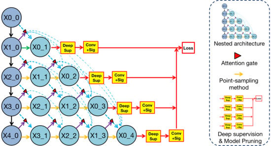
Figure 1.
Overview of methodologies in Render U-Net. Nested architecture is analyzed in
Section 3.1. Attention mechanism is analyzed in
Section 3.2. The point-sampling method is analyzed in
Section 3.3. Deep supervision is analyzed in
Section 3.4. Model pruning is analyzed in
Section 3.5.
Figure 1.
Overview of methodologies in Render U-Net. Nested architecture is analyzed in
Section 3.1. Attention mechanism is analyzed in
Section 3.2. The point-sampling method is analyzed in
Section 3.3. Deep supervision is analyzed in
Section 3.4. Model pruning is analyzed in
Section 3.5.
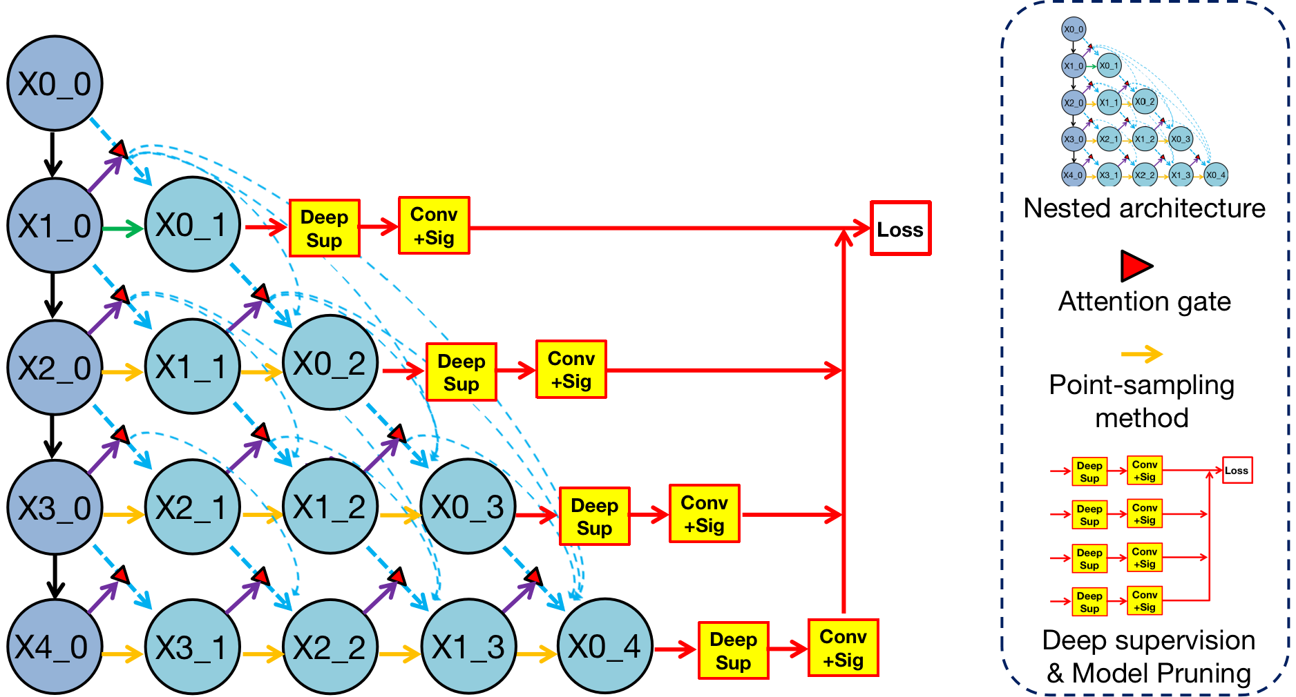
Figure 2.
Structure of Render U-Net. Every convolutional block captures features through two convolutional layers, which are activated by ReLU functions. From a horizontal perspective, all blocks are connected by dense skip connections with attention gates. Each block in the decoders concatenates multi-scale features from its all preceding blocks. Each block in the encoder transfers features from top to bottom through the maxpooling method from a vertical perspective, and each block in the decoder integrates multi-scale features across different resolutions through the point-sampling method. In addition, the block in deeper layer is sent to the attention gate as a gate signal.
Figure 3.
Diagram of Attention gate between convolutional block and . The feature of is used as a gate signal to focus regions in the encoder feature of . These two features are added after the convolution and BatchNorm layers.After activation by ReLU, the result is sent to the convolution and BatchNorm layers to extract features. Finally, the attention coefficient is obtained through the sigmoid function and then it dot-products, pixel by pixel, by using the upsampling feature to get the feature after attention selection, which is .
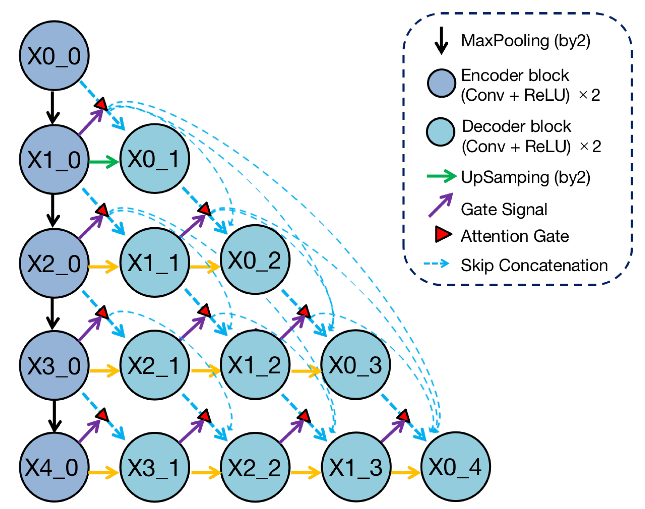
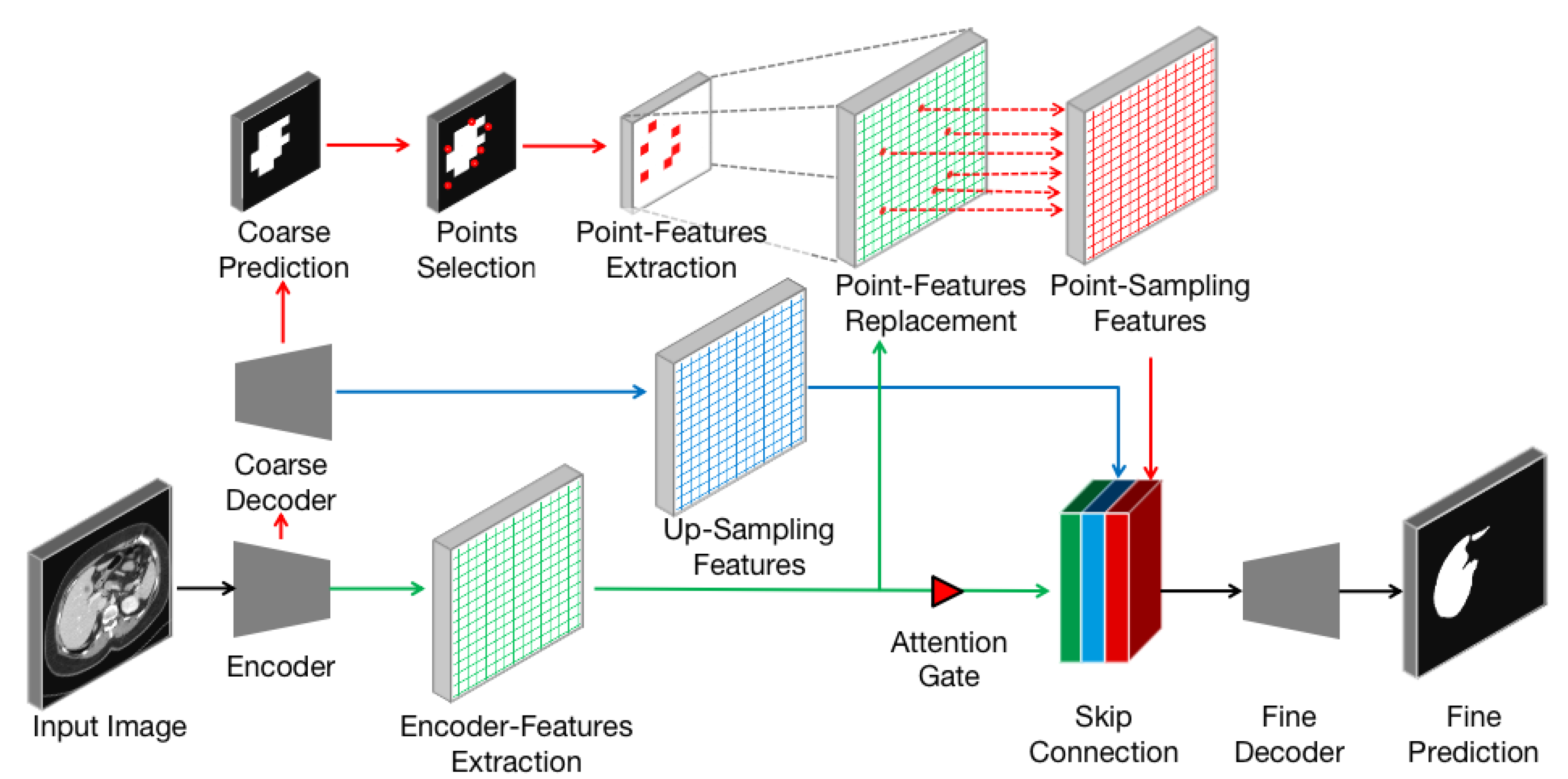
Figure 4.
Detailed analysis of the Point-sampling method (red arrows, dots, and grids) applied to image semantic segmentation. A set of uncertain points from coarse prediction is selected to extract point-features. These features will replace original upsampling features and concatenate to refine the boundary.
Figure 5.
Example of the coarse-to-fine process. First, a coarse mask on a 5 × 5 grid is predicted by the coarse decoder. Next, the N most uncertain points (dots in grids) are selected to recover detail on the finer grid. Finally, these point-features are extracted and then used to replace the original features extracted by the encoder.
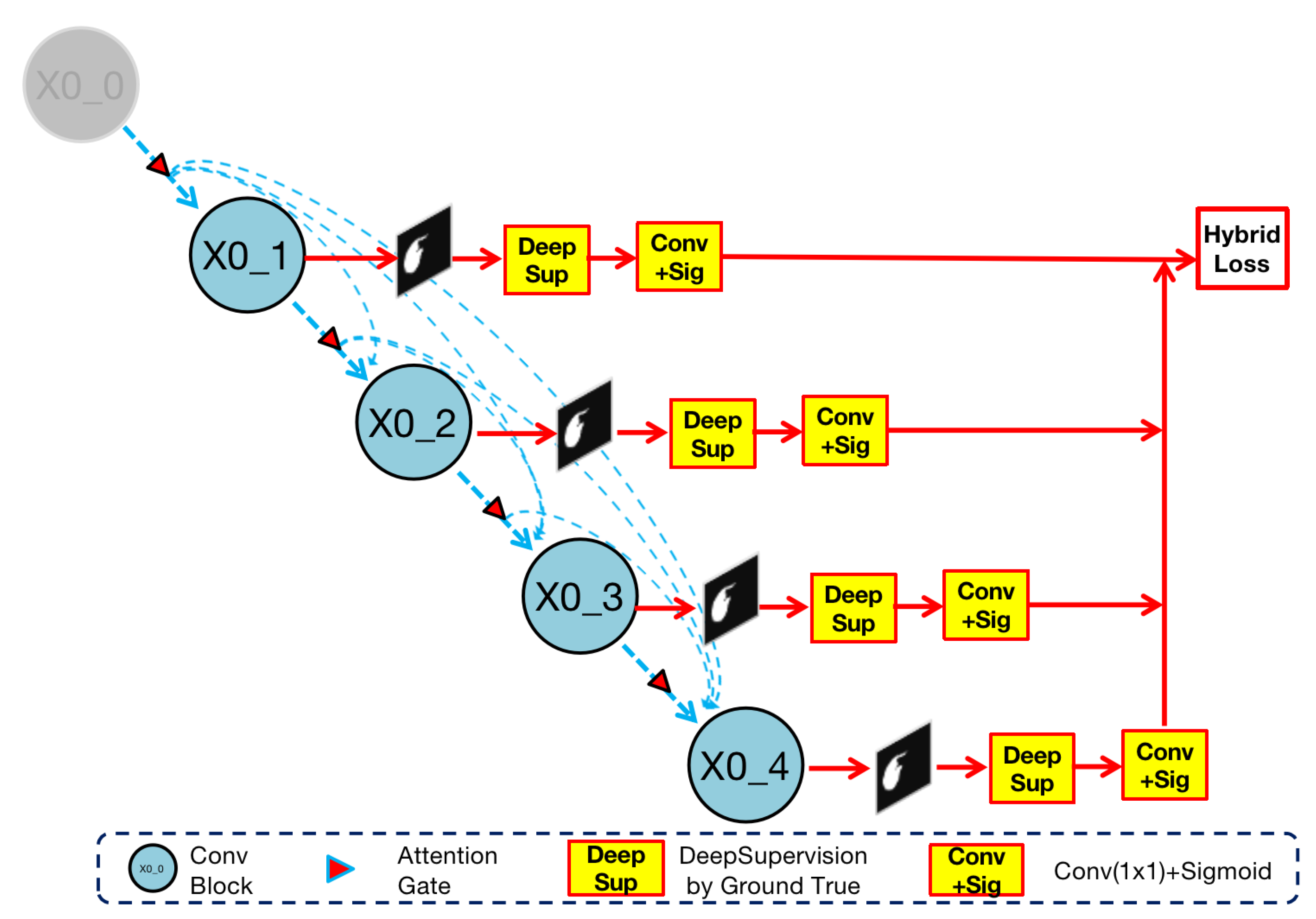
Figure 6.
Implementation of deep supervision in Render U-Net. Ground truth supervises the output of the nested convolution structure. The four results ,, , are compare with ground truth and directly participate in the calculation of hybrid loss.
Figure 6.
Implementation of deep supervision in Render U-Net. Ground truth supervises the output of the nested convolution structure. The four results ,, , are compare with ground truth and directly participate in the calculation of hybrid loss.
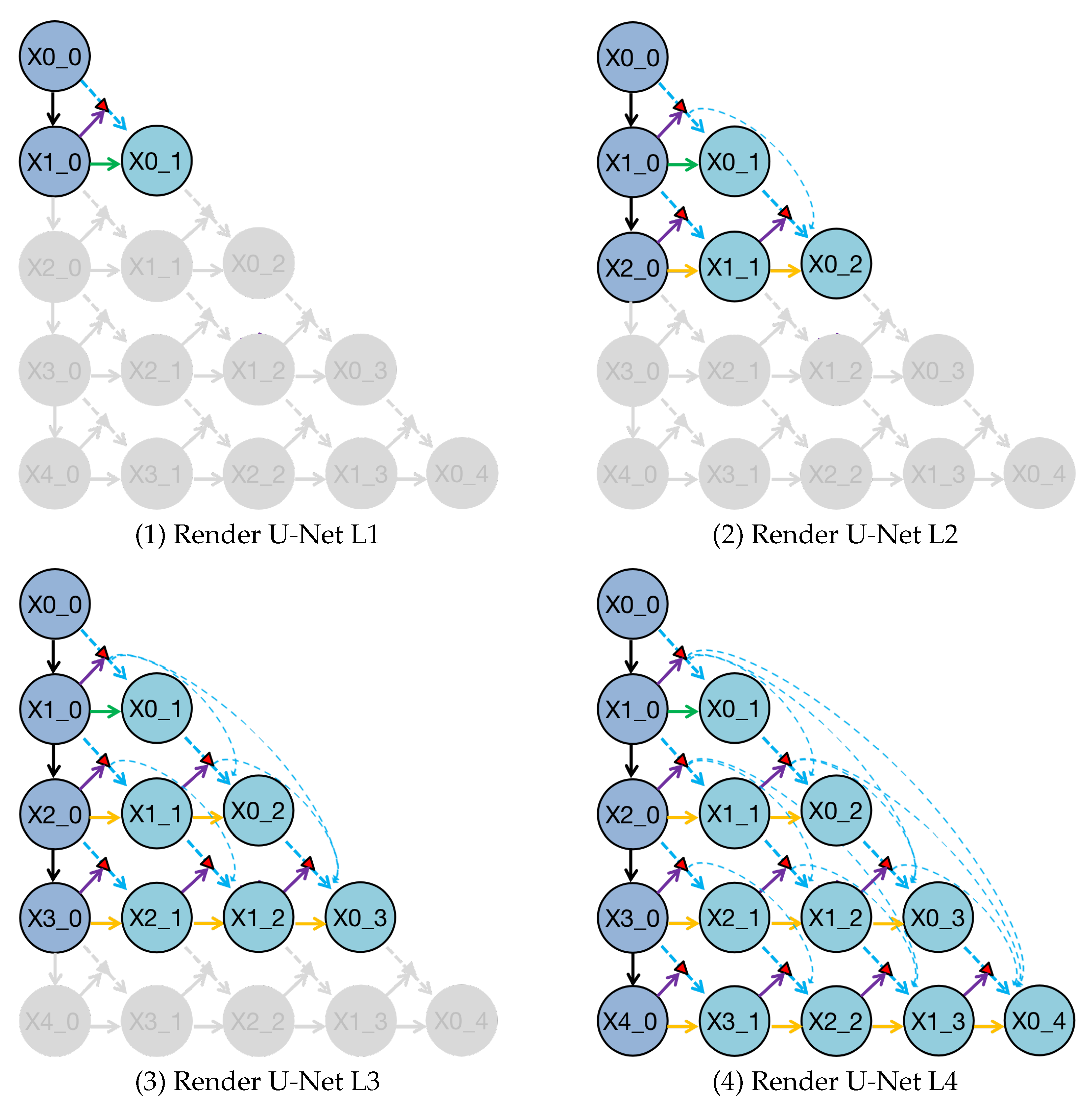
Figure 7.
Deep supervision helps the trained Render U-Net pruning at different depths to obtain four sub-networks, which are represented by Render U-Net L1, L2, L3, and L4. The gray components in these sub-networks have been deleted during inference.
Figure 7.
Deep supervision helps the trained Render U-Net pruning at different depths to obtain four sub-networks, which are represented by Render U-Net L1, L2, L3, and L4. The gray components in these sub-networks have been deleted during inference.
Figure 8.
Visualization and comparison of feature maps along skip connections for liver MRI images.
Figure 8.
Visualization and comparison of feature maps along skip connections for liver MRI images.
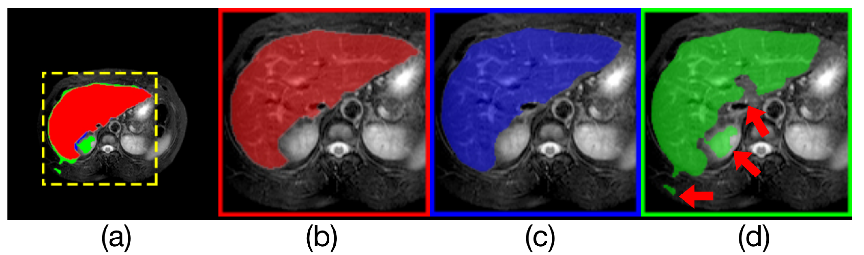
Figure 9.
Comparison of model outputs and ground truth. (a) shows the other three figures stacked from top to bottom, where the predicted extra areas are clearly seen. The red area in (b) is the manually annotated result. The blue region in (c) is the output of Render U-Net. The green region in (d) is the output of Attention U-Net. Some areas with incorrect predictions are indicated with red arrows in the figure.
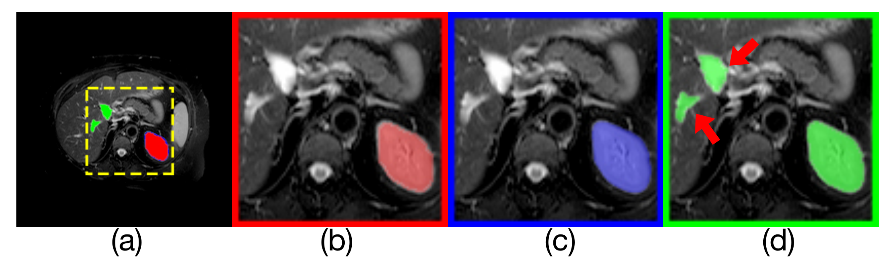
Figure 10.
Comparison of model outputs and ground truth. (a) is composed of the other three figures above are stacked from top to bottom, where the predicted extra areas are clearly seen. (b) is the manually annotated result. The blue region in(c) is the output of Render U-Net. The green region in (d) is the output of U-Net. Some areas with incorrect predictions are indicated with the red arrows in the figure.
Figure 11.
Comparison of model outputs and ground truth. (a) is composed of the other three figures above stacked from top to bottom, where the predicted extra areas are clearly seen. The red area in (b) is the manually annotated result. The blue region in (c) is the output of Render U-Net. The green region in (d) is the output of ANU-Net. Some areas with incorrect predictions are indicated with the red arrows in the figure.
Figure 12.
Comparison of model outputs and ground truth. (a) is composed of the other three figures above stacked from top to bottom, where the predicted extra areas are clearly seen. The red area in (b) is the manually annotated result. The blue region in (c) is the output of Render U-Net. The green region in (d) is the output of UNet++. Some areas with incorrect predictions are indicated with red arrows in the figure.
Figure 13.
Comparison of model outputs and ground truth. (a) is composed of the other three figures above stacked from top to bottom, where the predicted extra areas are clearly seen. The red area in (b) is the manually annotated result. The blue region in (c) is the output of Render U-Net. The green region in (d) is the output of UNet3+. Some areas with incorrect predictions are indicated with red arrows in the figure.
Figure 14.
The graph of the attention coefficient changing with training. The color change in the figures represents the change in the weight of attention learning, where red represents enhancement and blue represents inhibition. (a1–f1) is the first group of changes. (a2–f2) is the second group of changes. (a1,a2) are the input CT images. (b1,b2) are the ground truth of liver, respectively. (c1–f1) and Figure (c2–f2) are two groups of the attention coefficients in different training phases.
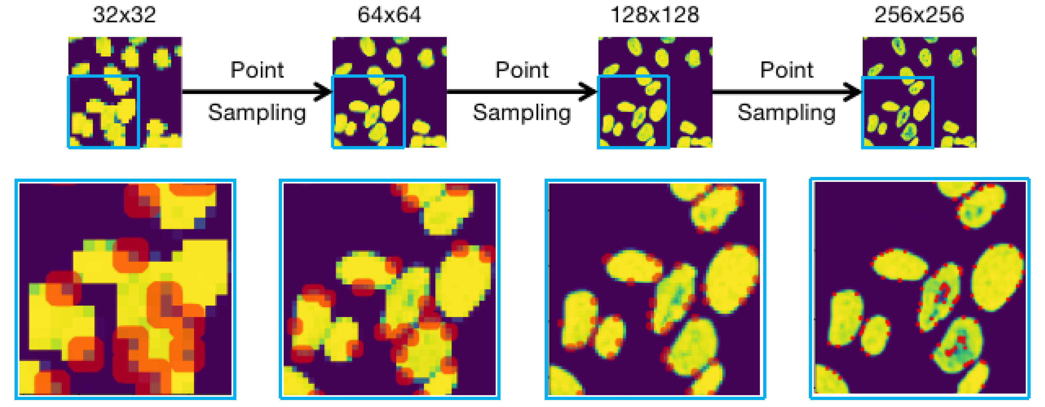
Figure 15.
Diagram of the Point-sampling process for rendering a higher resolution boundary when inferring nuclei. The red dots in different resolution are the selected uncertain points to calculate.
Figure 15.
Diagram of the Point-sampling process for rendering a higher resolution boundary when inferring nuclei. The red dots in different resolution are the selected uncertain points to calculate.
Figure 16.
Diagram of the relationships between the Dice coefficients and inference times of the four pruned Render U-Nets with segmentation of four kinds of objects. We use four blue circles with different areas to denote sub-networks with different parameter amounts.
Figure 16.
Diagram of the relationships between the Dice coefficients and inference times of the four pruned Render U-Nets with segmentation of four kinds of objects. We use four blue circles with different areas to denote sub-networks with different parameter amounts.
Table 1.
An overview of some important information of the medical image datasets used in this experiment.
Table 1.
An overview of some important information of the medical image datasets used in this experiment.
| Application | Resolution | Modality | Provider |
|---|
| Liver | 256 × 256 | CT | 2017 MICCAI LiTS |
| Spleen | 256 × 256 | MRI | 2019 ISBI CHAOS |
| Kidney | 256 × 256 | MRI | 2019 ISBI CHAOS |
| Liver | 256 × 256 | MRI | 2019 ISBI CHAOS |
| Nuclei | 96 × 96 | Mixed | 2018 DSB Kaggle |
Table 2.
The experiment results of the LiTS test dataset.
Table 2.
The experiment results of the LiTS test dataset.
| Models | mIoU | Dice | Precision (%) | Recall (%) |
|---|
| UNet [10] | 0.8949 | 0.9445 | 93.24 | 95.70 |
| R2UNet [17] | 0.9069 | 0.9511 | 93.80 | 96.48 |
| UNet++ [40] | 0.9446 | 0.9715 | 98.16 | 96.17 |
| PointUNet++ | 0.9655 | 0.9825 | 98.04 | 98.45 |
| UNet3+ [21] | 0.9784 | 0.9891 | 98.94 | 98.87 |
| AttentionUNet [24] | 0.9339 | 0.9658 | 96.79 | 96.37 |
| AttentionR2UNet | 0.9238 | 0.9603 | 97.12 | 94.98 |
| ANU-Net [20] | 0.9748 | 0.9815 | 98.15 | 99.31 |
| Render U-Net | 0.9823 | 0.9911 | 98.89 | 99.33 |
Table 3.
Performance of spleen segmentation for MRI images.
Table 3.
Performance of spleen segmentation for MRI images.
| Models | mIoU | Dice | Precision (%) | Recall (%) |
|---|
| UNet [10] | 0.7618 | 0.8648 | 82.34 | 91.06 |
| R2UNet [17] | 0.8150 | 0.8977 | 93.60 | 86.24 |
| UNet++ [40] | 0.8105 | 0.8953 | 86.37 | 92.93 |
| PointUNet++ | 0.9057 | 0.9502 | 97.70 | 92.50 |
| UNet3+ [21] | 0.8582 | 0.9235 | 94.77 | 90.18 |
| AttentionUNet [24] | 0.8413 | 0.9138 | 91.54 | 91.22 |
| AttentionR2UNet | 0.8162 | 0.8979 | 90.88 | 88.73 |
| ANU-Net [20] | 0.8923 | 0.8979 | 95.19 | 93.44 |
| Render U-Net | 0.9290 | 0.9629 | 97.32 | 95.35 |
Table 4.
Performance of liver segmentation for MRI images.
Table 4.
Performance of liver segmentation for MRI images.
| Models | mIoU | Dice | Precision (%) | Recall (%) |
|---|
| UNet [10] | 0.7537 | 0.8596 | 87.31 | 84.65 |
| R2UNet [17] | 0.7780 | 0.8750 | 92.11 | 83.39 |
| UNet++ [40] | 0.8423 | 0.9139 | 93.06 | 89.79 |
| PointUNet++ | 0.8551 | 0.9218 | 94.01 | 90.42 |
| UNet3+ [21] | 0.8224 | 0.9005 | 93.00 | 88.02 |
| AttentionUNet [24] | 0.7600 | 0.8637 | 91.11 | 82.09 |
| AttentionR2UNet | 0.8244 | 0.9035 | 94.74 | 86.40 |
| ANU-Net [20] | 0.8789 | 0.9355 | 94.23 | 92.88 |
| Render U-Net | 0.9056 | 0.9504 | 95.53 | 94.56 |
Table 5.
Performance of kidney segmentation for MRI images.
Table 5.
Performance of kidney segmentation for MRI images.
| Models | mIoU | Dice | Precision (%) | Recall (%) |
|---|
| UNet [10] | 0.8446 | 0.9158 | 89.20 | 94.08 |
| R2UNet [17] | 0.8554 | 0.9221 | 91.92 | 92.50 |
| UNet++ [40] | 0.8658 | 0.9281 | 90.87 | 94.82 |
| PointUNet++ | 0.8942 | 0.9442 | 92.66 | 96.24 |
| UNet3+ [21] | 0.8449 | 0.9155 | 89.91 | 93.44 |
| AttentionUNet [24] | 0.8577 | 0.9234 | 90.97 | 93.76 |
| AttentionR2UNet | 0.8734 | 0.9324 | 91.41 | 95.15 |
| ANU-Net [20] | 0.9010 | 0.9479 | 94.00 | 95.60 |
| Render U-Net | 0.9038 | 0.9494 | 94.14 | 95.77 |
Table 6.
Performance of nuclei segmentation by the models in the DSB test dataset.
Table 6.
Performance of nuclei segmentation by the models in the DSB test dataset.
| Models | mIoU | Dice | Precision (%) | Recall (%) |
|---|
| UNet [10] | 0.7909 | 0.8833 | 86.18 | 90.59 |
| R2UNet [17] | 0.6987 | 0.8199 | 81.23 | 82.77 |
| UNet++ [40] | 0.7028 | 0.8229 | 92.36 | 74.36 |
| PointUNet++ | 0.7507 | 0.8569 | 92.22 | 80.06 |
| UNet3+ [21] | 0.6853 | 0.8121 | 81.20 | 81.28 |
| AttentionUNet [24] | 0.7660 | 0.8675 | 85.81 | 87.71 |
| AttentionR2UNet | 0.7025 | 0.8235 | 89.85 | 76.16 |
| ANU-Net [20] | 0.8259 | 0.9003 | 91.42 | 89.77 |
| Render U-Net | 0.8360 | 0.9072 | 92.88 | 89.46 |
Table 7.
Hausdorff distance of five segmentation tasks.
Table 7.
Hausdorff distance of five segmentation tasks.
| Models | Liver (CT) | Spleen | Kidney | Liver (MRI) | Nuclei |
|---|
| UNet [10] | 14.95 | 11.94 | 11.87 | 30.98 | 35.54 |
| R2UNet [17] | 17.76 | 9.05 | 12.71 | 28.05 | 41.19 |
| UNet++ [40] | 9.31 | 7.82 | 11.97 | 25.59 | 34.05 |
| PointUNet++ | 7.62 | 6.32 | 10.53 | 23.12 | 32.32 |
| UNet3+ [21] | 6.36 | 7.25 | 13.13 | 23.97 | 37.21 |
| AttentionUNet [24] | 7.21 | 6.23 | 13.63 | 23.09 | 34.85 |
| AttentionR2UNet | 12.26 | 8.20 | 13.87 | 20.33 | 35.51 |
| ANU-Net [20] | 5.48 | 5.97 | 10.64 | 18.06 | 32.04 |
| Render U-Net | 4.41 | 5.39 | 10.49 | 16.96 | 31.65 |
Table 8.
Segmentation results of four pruned models. The inference time (counted by seconds) is calculated by segmenting 1K images.
Table 8.
Segmentation results of four pruned models. The inference time (counted by seconds) is calculated by segmenting 1K images.
| Model | Spleen | Kidney | Liver | Nuclei |
|---|
| Dice | mIoU | Time | Dice | mIoU | Time | Dice | mIoU | Time | Dice | mIoU | Time |
|---|
| L1 | 0.8258 | 0.7203 | 28.54 | 0.7588 | 0.6198 | 28.37 | 0.6624 | 0.5332 | 18.10 | 0.8490 | 0.7529 | 8.74 |
| L2 | 0.9272 | 0.8655 | 44.95 | 0.8519 | 0.7450 | 41.77 | 0.7546 | 0.6480 | 34.63 | 0.8516 | 0.7603 | 22.74 |
| L3 | 0.9451 | 0.8984 | 59.88 | 0.9353 | 0.8793 | 59.09 | 0.8797 | 0.8170 | 50.28 | 0.9072 | 0.8360 | 40.35 |
| L4 | 0.9629 | 0.9290 | 77.69 | 0.9494 | 0.9038 | 80.32 | 0.9056 | 0.9504 | 64.79 | 0.8864 | 0.8065 | 61.67 |


