Article

The New Approach to Analysis of Thin Isotropic Symmetrical Plates

Department of Mechanics Construction and Buildings Materials, Faculty of Civil, Architecture and Environmental Engineering, UTP University of Science and Technology, Al. prof. S. Kaliskiego 7, 85-796 Bydgoszcz, Poland
*
Author to whom correspondence should be addressed.
Appl. Sci. 2020, 10(17), 5931; https://doi.org/10.3390/app10175931
Submission received: 15 July 2020 / Revised: 20 August 2020 / Accepted: 23 August 2020 / Published: 27 August 2020
(This article belongs to the Special Issue Advances on Structural Engineering)

Abstract

:
A new approach to solve plate constructions using combined analytical and numerical methods has been developed in this paper. It is based on an exact solution of an equilibrium equation. The proposed mathematical model is implemented as a computer program in which known analytical formulae are rewritten as wrapper functions of two arguments. Partial derivatives are calculated using automatic differentiation. A solution of a system of linear equations is substituted to these functions and evaluated using the Einstein summation convention. The calculated results are presented and compared to other analytical and numerical ones. The boundary conditions are satisfied with high accuracy. The effectiveness of the present method is illustrated by examples of rectangular plates. The model can be extended with the ability to solve plates of any shape.

1. Introduction

Thin plates are widely used as elements of building and engineering structures. The Kirchhoff plate theory is the basis of engineering design and calculation of such elements. It is an approximate zeroth-order shear deformation plate theory. Discrepancy between order of basic differential equation and number of boundary conditions is the main disadvantage of the Kirchhoff theory. There are considered only three from six physical equations. Shearing and normal transverse stresses are not taken into account. They are determined from equation of equilibrium. The higher-order shear deformation plate theories are free from this discrepancy.
According to the Kirchhoff plate theory solution of thin isotropic plates is equivalent to solution of fourth-order partial differential equation [1,2]
2 2 w = q D ,
for given boundary conditions. In the above equation w is the deflection of the plate, and D is its flexural rigidity. Function q ( x 1 , x 2 ) describes distribution of load on upper surface of the plate. Uniform equation corresponds to (1) has the form
2 2 w = 0 .
In many cases, Kirchhoff theory gives satisfactory results and sufficient accuracy for practical purpose and correctly describes behavior of the structure. It is based on the linear distribution of the displacements through the plate thickness. As a result, parabolic distributions of the shearing stresses are obtained. For comparison Mindlin plate theory [3] also takes the same distribution of displacements but gives incorrect uniform distribution of the shearing stresses through the plate thickness. Higher-order theories like Christensen, Mindlin, Timoshenko can represent the kinematics better. However, they involve higher-order stress resultants that are difficult to interpret physically. Therefore, such theories should be used only when necessary [4]. In addition to its inherent simplicity and low computational cost, the first-order plate theory often provides a sufficiently accurate description of the global response for thin to moderately thick plates. Higher-order theories provide a small increase in accuracy relative to the first-order plate theory solution, at the expense of a significant increase in computational effort [5]. Therefore, the choice of the Kirchhoff theory to analysis of thin-walled engineering structures is still justified.
Let us note that exact solution of boundary problems of theory of the plates is possible only for simplest cases. At present, there are many various methods to solve thin plates, which can be divided into two basic groups: Analytical [2,6,7,8] and numerical ones [6,9,10,11].
Analytical methods are more exact than numerical methods but they allow the solving of boundary problems of plates with a small number of unknown parameters and constrained by canonical contour as rectangle, square, triangle, circle or ellipse. Numerical methods are less exact but they allow the solving of arbitrary configuration plates [12] at the expense of a significant increasing of unknown parameters. It increases the time for calculations and leads to the accumulation of computational errors.
Numerical methods are currently reaching their limits. Among numerical methods, the Finite Element Method (FEM) [13,14] and Finite Boundary Method (FBM) [15,16,17,18] are the most common. The finite element method allows us to approximately solve plate of arbitrary configuration, where the analytical solution is impossible. Research on this method can be conventionally divided into: theoretical (related the construction of finite element model) and applied (related to the use of the method to solve complicated technical problems).
In recent years, many methods which are free from disadvantages of standard numerical ones have been suggested. They create separate group called analytical-numerical methods. According to these methods part of equations are performed in analytical manner and others with help of numerical procedures. The method suggested in present paper belongs to this group. Differences compared to numerical methods:
  • Simplicity of structure modeling. Equations of equilibrium are solved once independently of the boundary conditions and solution remains unchanged throughout the calculation process. This allows the reduction of structure modeling to set kinematic and static boundary conditions in the separate points at the plate contour.
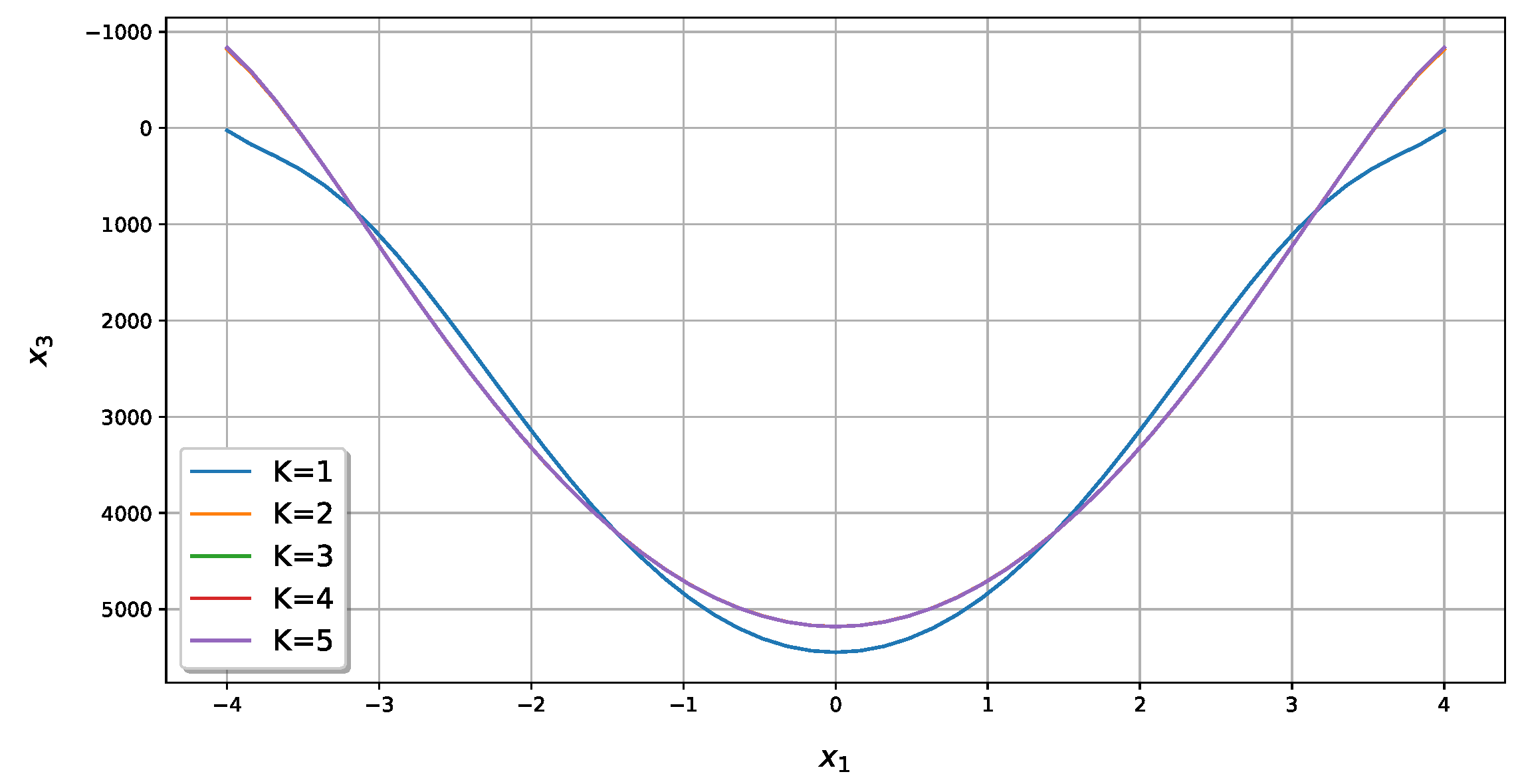
  • Possibility to provide better accuracy in comparison with finite element method. It is achieved only by increasing of number of the approximations (parameter K) or replace nodes at the contour. This procedure is performed automatically with author’s program to solve of the plate structure.
  • Possibility to define the load as a function of two variables. Because not all FEA programs provide such functionality, ABAQUS software have been chosen to compare the results.
  • Possibility of implementing of suggested method in higher-order theory, say Mindlin-Reissner theory.
The mathematical model proposed in the article has been implemented as a computer program which is characterized by a readable and concise source code (Appendix B). This method requires much less computation operations to solve the structure in comparison to FEM. There is no need to:
  • Discretize of the structure into set of finite elements,
  • Aggregate of this set into discrete structure,
  • Introduce local and global coordinate system,
  • Numerate of nodes. Solution of equilibrium equation can be obtained with given accuracy and it is independent of the number of approximations.
In contrast to FEM, the suggested method uses essentially fewer equations to solve the structure. Owing to high accuracy of solution of equilibrium equation we need fewer nodes to satisfy boundary conditions. These nodes are placed only at the contour.
There are four main techniques to calculate derivatives in the literature [19]: hand-coded analytical derivatives, numerical differentiation, symbolic differentiation and automatic differentiation. Hand-coded analytical derivatives are exact but time consuming to code, error prone and not automated. Numerical differentiation is easy to code. However, as an estimation approach, it is known to produce inaccurate results. Symbolic differentiation is a technique for computing derivatives of mathematical expressions via symbolic manipulation. This technique is used by computer algebra systems. It is exact, but memory intensive and slow.
In author’s computer program automatic differentiation (AD) is used, because it is free from the drawbacks of techniques described above. Unlike symbolic differentiation, which operates on mathematical expressions, automatic differentiation operates on code. Automatic differentiation leverages the chain-rule-based for evaluating the derivatives. It is exact and speed in comparable to hand-coded derivatives. We calculate higher-order derivatives using autograd library. Finally, using jax [20]—the successor of the autograd library—it is possible to run our Python and NumPy programs not only on CPUs (central processing units) but also on much more efficient GPUs (graphics processing units) and TPUs (tensor processing units). Therefore, significant acceleration of calculations can be expected.
The purpose of this paper is construction of effective analytical-numerical method to solve of thin symmetrical plates. The suggested method is based on continuum material model. General solution of equation of equilibrium (1) is presented as sum of general solution of uniform Equation (2) and particular solution of non-uniform Equation (1). They are independent between themselves and contain theoretically infinite number of unknown parameters which allow the performance of the equation of equilibrium and boundary conditions with given accuracy.
General solution of equilibrium equation includes functions of shape of deflection. Functions of shape of displacements, moments, shearing forces and generalized shearing forces have been obtained using automatic differentiation. Such structure of solution allows easily to model various boundary conditions. Obtained relations create the mathematical model of a plate.
Equation of equilibrium is performed by collocation method in each point on the plate surface which are called surface nodes. They are not vertexes of finite element. Improvement of accuracy of solution is achieved by increasing of unknown parameters with author’s program. General solution of Equation (2) contains separate unknown coefficients which allow the performance of boundary conditions written in the points at the plate contour. They are called edge nodes. author’s program fulfils generation of edge and surface nodes and their distribution.
To obtain solution of the plate with proposed method we at first perform equation of equilibrium in the separate points on the plate surface and obtain particular solution of the problem. Next, we expect that this solution is unchanged and satisfy boundary conditions in the separate points at the plate contour.

2. Literature Review of the Methods for Solving Plate Bending Problems

Exact solution of the boundary problems of the plate theory are possible only for simplest cases. So far, many methods of approximate solution of plates have been developed. All of them can be divided into two basic groups: Analytical [1,2,6,7] and numerical ones [2,9,10,15]. Their analysis is given in fundamental monograph by editor Czeslaw Wozniak [21].
Formulation of the problem of the plate theory usually is performed one of the three techniques: system of equilibrium differential equations, variation approach and method of integral equations.
Solution of differential equations of equilibrium causes development of analytical methods. Numerical methods are less exact but they allow the solving of arbitrary configuration plates [2,10] at the expense of a significant increasing the number of unknowns. It increases the time for calculations and leads to accumulation of computational errors.
Analytical methods include: Ritz-Timoshenko [8], Bubnov-Galerkin [22] and other [23] variational methods, Navier’s [24] method of single and double trigonometric series, Lévy’s method of functional series [1,8,25] and spline-function method [26,27] which is widely used for solution of the plate with discontinuous configuration.
Ritz-Timoshenko method is based on the principle of minimum of the structure potential energy (Principle of Virtual Works).
δ Π = δ ( V A ) = 0 ,
Here Π is potential energy of the structure; V—specific potential energy; A is work of outer load applied to plate structure; δ —Lagrange variation symbol.
Minimalization of error R of approximate solution of Equation (4)
D 2 2 w q = R 0 ,
with respect to test functions is object of Bubnov-Galerkin method.
Navier’s method only deals with rectangular plate free supported at the contour and arbitrary loaded. Lévy’s method allows the solving of the plates with two opposite edges free supported. Other edges can be arbitrary fixed.
Numerical methods includes: method of boundary collocation [9,28] and Trefftz collocation method [13,29], finite element method (FEM) [14,30,31,32,33,34], finite boundary method (FBM) [15,17,18] and method of time-space elements (MTSE) [35].
Method of boundary collocation demands satisfaction of integral equations and Trefftz collocation method demands to perform equilibrium equation. In both methods, the boundary conditions are performed at separate points called collocation points at the edges of the plate. Trefftz method does not contain singular integrals and it is more exact in comparison with other methods. Variant of collocation method is worked in paper [36] for a plate inscribed in rectangular contour. Collocation points are Chebyshev nodes. The authors argue that with the number of computational nodes increasing, the accuracy is not improved because of the round-off error effect.
Finite element method (FEM) follows from variation formulation and finite boundary method (FBM) does from boundary integral equation. In the paper [34] four nodal plate element based on Reissner-Mindlin plate theory is worked. Mesh refinement increase the accuracy of the solution. Finite element modeling of stiffened and unstiffened orthotropic plates is presented in the paper [37].
In recent years, besides numerical and analytical methods, many analytical-numerical ones appear. There are: boundary integral method (BIM) or boundary integral equation method [17], global element method (GEM) [38] and global-local finite element method (GLFEM) [11], spline finite element method [39], scaled boundary finite element method [40], least squares collocation method [41], symplectic superposition method [42] and matrix method [43].
BIM is part of general method BEM associated with calculation singular integrals containing in BEM. According to global element method (GEM) [38] considered area is divided into some simple subareas (greater than in FEM). Division is defined by configuration of the area, solution typologies and mechanical properties of material. In each area approximate functions are taken as linear combinations of polynomial, trigonometric and exponential functions. For example, linear global or superelement has three degrees of freedom. Interpolation functions are taken in the form of second order polynomial. Boundary and continuity conditions at the common edges of the subareas are performed in manner of principle of virtual work. Fault of the method is difficulty of division of considered area into elements and selection of the functional for minimization.
Global-local finite element method (GLFEM) [11] uses Ritz-Timoshenko method at the one part of the plate and finite element method at the another. Fault of this method is necessity of individual treatment of each problem and unstudied effectiveness. According to this method structure is first analyzed as a whole. Therefore, all the local details obtained from the global analysis are considered to be boundary conditions in local details analysis. The global-local analysis is especially useful in the stress concentration analysis, and so on. More information on global-local finite element method can be found in [44,45,46,47,48].
The extended finite element method (G/XFEM) [3,49,50,51,52,53,54,55] is generalization of classical finite element method and it was especially developed for modeling structural problems with discontinuities. According to that generalized global approximation of the deflection of the plate is presented as [51]:
u ˜ ( x ) = j = 1 N N j ( x ) u j standard interpolation + j = 1 N N j ( x ) i = 2 q L j i ( x ) b j i enriched interpolation
where u j is a nodal parameter associated with finite element shape functions N j ( x ) , b j i are nodal parameters associated with G/XFEM shape functions— N j ( x ) · L j i ( x ) . L j i are so-called enrichments functions that hold the information about the problem solution.
In the last ten years, there has been a growing interest in meshless methods [56,57]. These methods do not demand of mesh as finite element ones. Area discretization is accomplished by a set of ordered or scattered nodes that are independent of the plate configuration. This approach does not cause difficulties in satisfying boundary conditions. The method is a simply, effective and attractive.
Novel plate and shell analysis methods also include analysis of the Kirchhoff plate using rational Bézier triangles in isogeometric analysis coupled with a feature-preserving automatic meshing algorithm [58] and modeling using a NURBS-based isogeometric analysis (IGA) approach [59].
Some results obtained by analytical and numerical methods are given below. Rectangular uniformly loaded plate free supported at two opposite edges or rigidly clamped at the contour is considered in the paper [60]. To solution the problem Lévy’s method was used here. In each concrete case particular solution is taken separately. In similar manner the same plate free supported at the corners was considered in the paper [61].
The exact solution of orthotropic rectangular cantilever arbitrary loaded plate is obtained in [62]. Rectangular plate free supported at the contour was solved [63] using Bubnov-Galerkin variation method. Various kinds of outer load were considered. Using combination of functional series S. Timoshenko obtained original analytical solution of thin orthotropic plate rigidly clamped at the contour [8]. Krjukov using spline approximation method obtained solution of parallelogram and trapeze plates [26].
Trefftz method boundary collocation was used to solve thin anisotropy plate of various geometry [29]. The obtained results are in perfect agreement with known analytical and numerical solutions. Thin rectangular cantilever plate [28] and irregular thin plate on Winkler foundation [36] were also solved with this method.
Finite element method was used [64] to solve the anisotropic elastic plates with holes and cracks.
Method of boundary equations is applied to bending problem of the thin plate [65]. Plate is supported on the columns. Substitute forces at the edges and concentrated forces in the corners are not introduced in the given formulation. The problem was solved by boundary integral equations method. Collocation points were placed outside of the plate. This approach allowed to eliminate singular integrals in calculation.
Bending analysis of rectangular moderately thick plates with spline finite element method is subject of the paper [39]. Analysis of deflection of regular and irregular plates with matrix method is fulfilled in the paper [43].
Boundary element method was used to solve stiffened plates [37]. Elastic bending problem of such plates were investigated with boundary element method [66].
Fracture mechanics problems for plane stress and plane strain state solved with extended finite element method is considered in the paper [51]. With help of this method Reissner-Mindlin cracked plate was solved [3]. In article [67] bending by concentrated force of a cantilever strip with a through-thickness crack perpendicular to its axis was solved using linear conjunction method.
The new analytical-numerical method to analysis of symmetric Kirchhoff plate is presented in this paper. The method combines the advantages of an analytical (Navier and Lévy) as well as numerical (Trefftz collocation and finite element) methods. Equation of equilibrium is performed exactly in whole area within the plate. Kinematic and static boundary conditions are satisfied only at the separate nodes at the plate edges with the high accuracy.
The suggested method is close to Trefftz collocation method and meshless ones. It was tested on examples of cantilever plate [68], isotropic irregular plate [69], orthotropic plate resting on Winkler’s foundation [70,71], double-connected isotropic rectangular plates [71] and plate connected with truss [72]. Its improved version is given in the presented paper. Polynomial which was introduced in our previous publications for improvement of calculation results has been removed here as unnecessary.

3. Materials and Methods

Plate is a body constrained by two parallel planes and lateral surface. Upper and bottom planes are bases of the plate. Plane equidistant from the bases is called middle plane. Line of the cross-section middle plane with lateral surface is plate contour. Further we will be designate plate P, surface S and contour C and we take into account the assumptions proposed by Kirchhoff.
Let us consider thin isotropic symmetrical plate with at least two symmetry axes which has thickness h and surface S. Plate is referred to right-handed Cartesian coordinate system O x 1 x 2 origin at its geometrical center and constrained by contour C (Figure 1a). We assume that it is balanced with outer load q ( x 1 , x 2 ) applied to surface S and complied with the boundary conditions. Symmetry of the plate geometry, mechanical properties, boundary conditions and outer load are taken into account in this paper. Plate is defined by coordinates of its vertices V i ( ξ i , η i ) , i = 1 , , n .
We choose the solution of Equation (1) in the form of sum of general solution w 0 of uniform Equation (2) and particular solution w * of Equation (1).
w = w 0 + w * .
General solution of Equation (2) we take in the following form [73].
w 0 = f k p s ( x s ) · T k p ( 3 s ) ( x 3 s ) .
Einstein summation rule is used here. According to this convention indices repeated twice in a single term imply the summation is to be done. Summation indices in formula (7) are k, p and s. As particular cases, we obtain Lévy ( p = 1 , s = 2 ) and Timoshenko ( p = 1 , s = 1 , 2 ) forms of representation. In the above p = 1 , 2 ; s = 1 , 2 ; k = 1 , , K , where K is several approximations of the solution and determines its accuracy. The K is greater the accuracy of the solution is better.
T k p s ( x s ) are given trigonometric functions
T k 1 s ( x s ) = cos γ k s x s ; T k 2 s ( x s ) = cos δ k s x s .
Here
γ k s = k π a s ; δ k s = ( 2 k 1 ) π 2 a s .
Parameters a s ( s = 1 , 2 ) are model constants. They must be given a priori. In suggested model they are taken as sizes 2 a s ( s = 1 , 2 ) of rectangular contour L described on plate contour C (Figure 1b).
Unknown functions f k p s ( x s ) we take in the form
f k p s ( x s ) = R k p s E k p s ( x s ) .
Because indices k, p, s appear at the both sides of this formula, summation according to these indices does not perform.
In the above R k p s are unknown coefficients which are determined from boundary conditions at the plate contour, E k p s ( x s ) are unknown functions. Substituting expressions (7)–(10) into Equation (2) we come to system of two unbounded forth order homogeneous differential equations with respect to these functions [70].
E k p 1 ( I V ) ( x 1 ) 2 κ k p 2 2 E k p 1 ( x 1 ) + κ k p 2 4 E k p 1 ( x 1 ) = 0 ; E k p 2 ( I V ) ( x 2 ) 2 κ k p 1 2 E k p 2 ( x 2 ) + κ k p 1 4 E k p 2 ( x 2 ) = 0 ;
where
κ k p s = γ k s , p = 1 , δ k s , p = 2 .
Functions E k p s ( x s ) are taken as the following
E k p s ( x s ) = exp λ k p s x s .
Substituting expression (13) into Equation (11) we come to system of characteristic equations
λ k p 1 4 2 κ k p 2 2 λ k p 1 2 + κ k p 2 4 = 0 , λ k p 2 4 2 κ k p 1 2 λ k p 1 2 + κ k p 1 4 = 0 .
Let λ k p s ν , where ν = 1 , 2 be their roots. Then functions f k p s ( x s ) take the form [69]
f k p s ( x s ) = R k p s ν B k p s ν ( x s ) ,
In the above
B k p s 1 ( x s ) = cosh κ k p ( 3 s ) x s exp κ k p ( 3 s ) a s , B k p s 2 ( x s ) = x s sinh κ k p ( 3 s ) x s a s exp κ k p ( 3 s ) a s ,
Functions B k p s ν ( x s ) are called the basic functions of the solution.
According to (10) general solution of Equation (2) takes the form
w 0 ( x 1 , x 2 ) = R k p s ν · W k p s ν ( x 1 , x 2 ) .
Functions
W k p s ν ( x 1 , x 2 ) = B k p s ν ( x s ) · T k p ( 3 s ) ( x 3 s )
are dependent on the solution of the problem and are called shape functions of the plate deflection.
General solution of Equation (1) we obtain substituting (17) into expression (6)
w ( x 1 , x 2 ) = R k p s ν W k p s ν ( x 1 , x 2 ) + W * ( x 1 , x 2 ) .
Here W * ( x 1 , x 2 ) = w * ( x 1 , x 2 ) is particular solution of equation (1). Functions W * ( x 1 , x 2 ) can be present in the form:
W * ( x 1 , x 2 ) = C m n p q · W m n p q ( x 1 , x 2 ) .
Functions W m n p q ( x 1 , x 2 ) are dependent on outer load and called force functions of the plate deflection. For each specific problem they can be obtain using special procedures.
With the deflection of the plate w and using relations known from theory of thin isotropic plates, we obtain the expressions for tangent displacements [71,72]
u 1 ( x 1 , x 2 ) = R k p s ν U k p s ν ( x 1 , x 2 ) + U * ( x 1 , x 2 ) , u 2 ( x 1 , x 2 ) = R k p s ν V k p s ν ( x 1 , x 2 ) + V * ( x 1 , x 2 ) ,
moments
M 11 ( x 1 , x 2 ) = R k p s ν X k p s ν ( x 1 , x 2 ) + X * ( x 1 , x 2 ) , M 22 ( x 1 , x 2 ) = R k p s ν Y k p s ν ( x 1 , x 2 ) + Y * ( x 1 , x 2 ) , M 12 ( x 1 , x 2 ) = R k p s ν Z k p s ν ( x 1 , x 2 ) + Z * ( x 1 , x 2 ) ,
shearing forces
Q 1 ( x 1 , x 2 ) = R k p s ν H k p s ν ( x 1 , x 2 ) + H * ( x 1 , x 2 ) , Q 2 ( x 1 , x 2 ) = R k p s ν G k p s ν ( x 1 , x 2 ) + G * ( x 1 , x 2 ) ,
and generalized shearing forces
V 1 ( x 1 , x 2 ) = R k p s ν K k p s ν ( x 1 , x 2 ) + K * ( x 1 , x 2 ) , V 2 ( x 1 , x 2 ) = R k p s ν L k p s ν ( x 1 , x 2 ) + L * ( x 1 , x 2 ) .
In the above functions U k p s ν , V k p s ν , and so on are partial derivatives of shape functions W k p s ν . Similarly functions U * , V * , etc. are partial derivatives of force functions W * . They have been calculated using automatic differentiation [19,74].
Expressions (19)–(24) constitute mathematical model of considered plate. According to this model plate is in internal equilibrium with outer load q ( x 1 , x 2 ) , but boundary conditions are not satisfied here. Unknown coefficients R k p s ν are degrees of freedom of the plate. They are determined satisfying boundary conditions at the separate points of the contour. Let us consider technique of their generation.
Due to the symmetry of the plate, we can consider only its quarter. At first, we introduce two sets X 1 and X 2 of points ( x 1 m , x 2 n ) with numbers ( m , n ) placed at the positive semi axes of the plate and called them initial points.
Projections of these points onto the contour C are called current nodes and designated K r m and L r n correspondingly, where r is number of the edge (Figure 1b). It is seen that edges parallel to coordinate axes contain current nodes generated by either set X 1 or set X 2 but nodes placed at the inclined edge are generated as set X 1 so X 2 . If two initial points of set X 1 and X 2 fall into one node at the inclined edge we have double current node. Projections of these points into the vertex V i , with number i we call corner nodes and designated K ¯ i r , L ¯ i r  [69]. Union of current and corner nodes we called edge nodes.
Let us consider for simplicity rectangular plate (Figure 2). Its contour has no double nodes. In this case, we can say that each edge node is generated by single initial point. From this reason each function f 1 p s ( x s ) corresponds to single initial point. At each edge node two boundary conditions are written.
Corner nodes, say K ¯ 32 and L ¯ 33 , have the same coordinates ( a 1 , a 2 ) but they lie at the different edges of the normals n 2 and n 3 . Thus, they are different nodes. Each edge node is generated by single initial point. At the first approximation ( K = 1 ) we have eight unknown coefficients R 1 p s ν . Thus, eight boundary conditions written at four edge nodes can be satisfied. To that four initial points must be chosen at the semi coordinates axes ( x 1 m = 1 , 2 ; x 2 n = 1 , 2 ) . Following for approximation K there must be 2 K points x 1 m = 1 , , 2 K ; x 2 n = 1 , , 2 K . For illustration of effectiveness of the proposed method as an example we consider rectangular plate (Figure 2) with thickness h and plane sizes 2 a s ( s = 1 , 2 ) . This example allows easily compares author’s results with results obtained by other available methods.
To obtain the particular solution w * of Equation (1) we present outer load q ( x 1 , x 2 ) in the form of double trigonometric series [70,73]
q ( x 1 , x 2 ) = q m n p q · T m p 1 ( x 1 ) · T n q 2 ( x 2 ) , m , n = 1 , 2 , 3 ,
For rectangular plates parameters q m n p q can be determined as coefficients of expansion of the outer load in Fourier series on the surface of the plate. New symbols have been introduced here.
T m 1 s ( x s ) = cos γ m s x s ; T m 2 s ( x s ) = cos δ m s x s ;
γ m s = m π a s ; δ m s = ( 2 m 1 ) π 2 a s .
For rectangular plates force functions W m n p q are taken in the form
W m n p q ( x 1 , x 2 ) = T m p 1 ( x 1 ) · T n q 2 ( x 2 ) . p , q = 1 , 2
Substituting expressions (25), (28) into Equation (1) with taking into account (19,20) and equating coefficients at the same expressions in the both sides of Equation (1) we find coefficients C m n p q expressed by outer load.

4. Results

Let us consider three kinds of rectangular plates under various boundary conditions:
1
Rectangular plate with two opposite edges simply supported and the other free,
2
Rectangular plate simply supported at the contour,
3
Plate clamped at the contour.
Plates are loaded by particular load
q = C · cos δ 1 x 1 · cos δ 2 x 2
where
δ s = π 2 a s
and
C = q 0 D δ 1 2 + δ 2 2 2 .
Here q 0 = 10 k Pa is intensity of the load.
During the calculations the following geometric and mechanical parameters of model were take into consideration: plate sizes 2 a 1 = 8 m , 2 a 2 = 4 m , thickness h = 0.2 m . Young’s modulus is equal to E = 30 × 10 9 Pa and Poisson ratio ν = 0.2 .
The problem has been solved in third approximation ( K = 3 ) using 12 initial points. Consequently, we have 12 edge nodes. Distribution of initial points for ( K = 3 ) approximation is given in table:
x 1 m 0.00.81.62.43.24.0
x 2 n 0.00.40.81.21.62.0
Performed calculations have shown that increasing the K value for rectangular plates no longer affects the accuracy of the solution. It means that an exact solution is already obtained for small K. This confirms the high effectiveness of this method.
The results obtained using a Python-based computer program implementing the considered mathematical model have been compared with the analytical solution presented by Timoshenko and the numerical solution obtained with the Finite Element Method in the ABAQUS CAE program (Student Edition 2019 restricted to 1000 nodes), which allows defining the load as a function of two variables. ABAQUS model used for comparison consists of 512 S4R elements ( 561 nodes).
Due to symmetry of the problem deflection w ( x 1 , x 2 ) and the moments M 11 ( x 1 , x 2 ) , M 22 ( x 1 , x 2 ) are symmetrical functions of variable ( x 1 , x 2 ), while slops φ 1 ( x 1 , x 2 ) and φ 2 ( x 1 , x 2 ) are antisymmetrical ones.

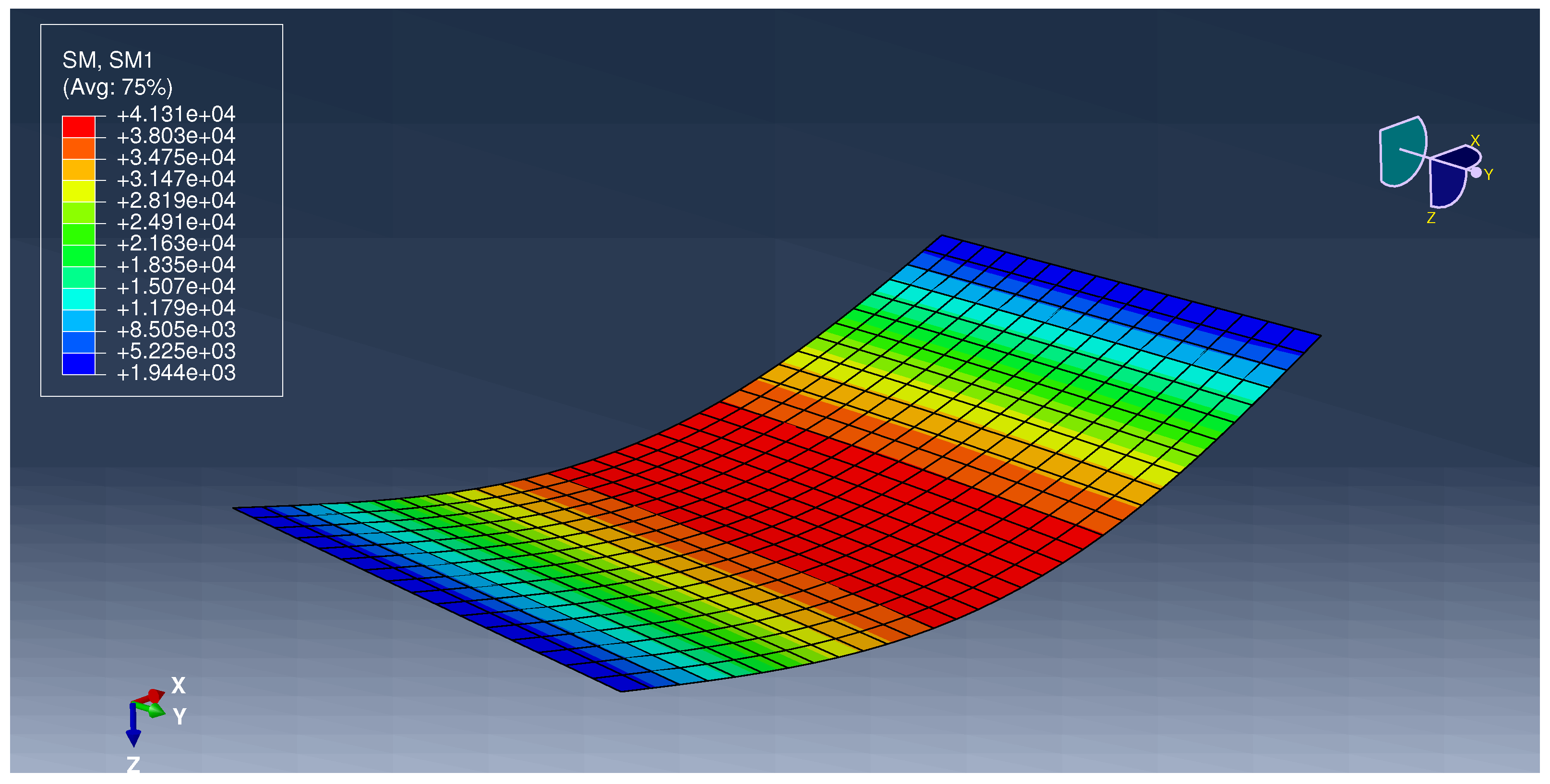
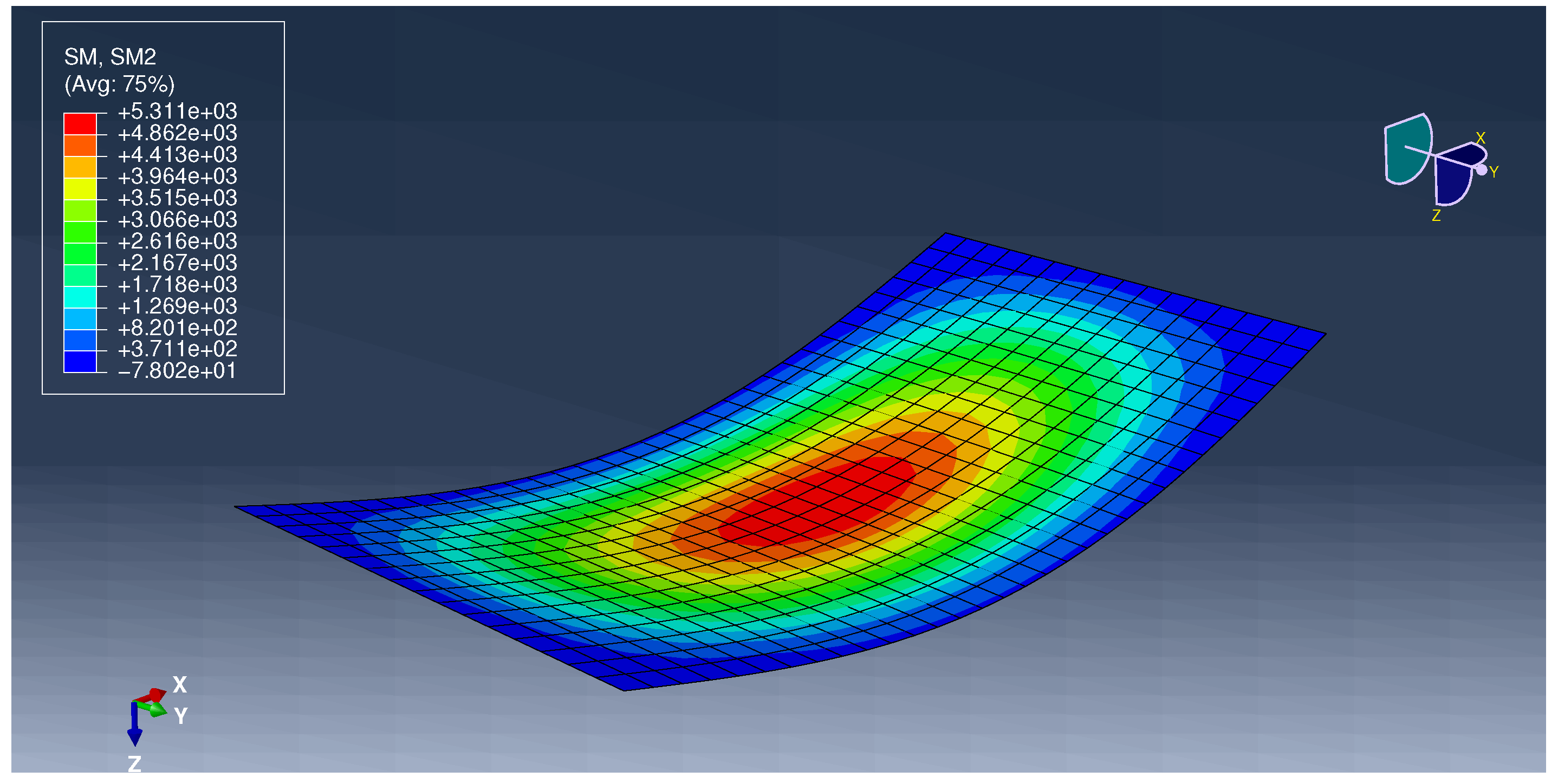
4.1. Rectangular Plate with Two Opposite Edges Simply Supported and the Other Free

Following boundary conditions must be satisfied (see Figure 3)
w ( x 1 , x 2 ) | x 1 = ± a 1 = 0 ; M 11 ( x 1 , x 2 ) | x 1 = ± a 1 = 0 ; M 22 ( x 1 , x 2 ) | x 2 = ± a 2 = 0 ; V 2 ( x 1 , x 2 ) | x 2 = ± a 2 = 0 .
Three-dimensional plots of deflection w and bending moments M 11 , M 22 in rectangular plate with discontinuous boundary conditions are given in Figure 4, Figure 5 and Figure 6.
Figure 7, Figure 8, Figure 9, Figure 10 and Figure 11 show cross-sectional plots of these magnitudes.
At the middle (Figure 7) and edge (Figure 8) sections deflections of the plate are almost the same. It means that considered plate under given conditions works as a simple beam.
Bending moment M 11 at the middle cross-section (Figure 10) is essentially greater than moment M 22 at this section (Figure 11). Bending moment M 22 and generalized shearing force V 2 are almost zero at the whole simply supported edges ( x 2 = ± a 2 ) . At the simply supported edges ( x 1 = ± a 1 ) deflection and slope φ 2 are also zero (values of the order of 1 × 10⁻¹⁸ and 1 × 10⁻¹⁷). All boundary conditions are performed at the current and corner nodes.
Extreme values of these variables are collected in Table 1. The maximum values are close to the maximum values obtained in the ABAQUS package (Appendix A.1), but the minimum ones for bending moments do not coincide.
Minimum values for the bending moments in the presented examples are values on the edge. Similar observations concerning the comparison of the FEM (ABAQUS) results were included in other works, e.g., in [75,76] where it was indicated that FEM is unable to meet the zero-bending moment at the edge. The explanation of the reason for discrepancy between present method and FEM is included in the Discussion.
Compliance with boundary conditions in the midpoints at the edges is presented in Table 2.

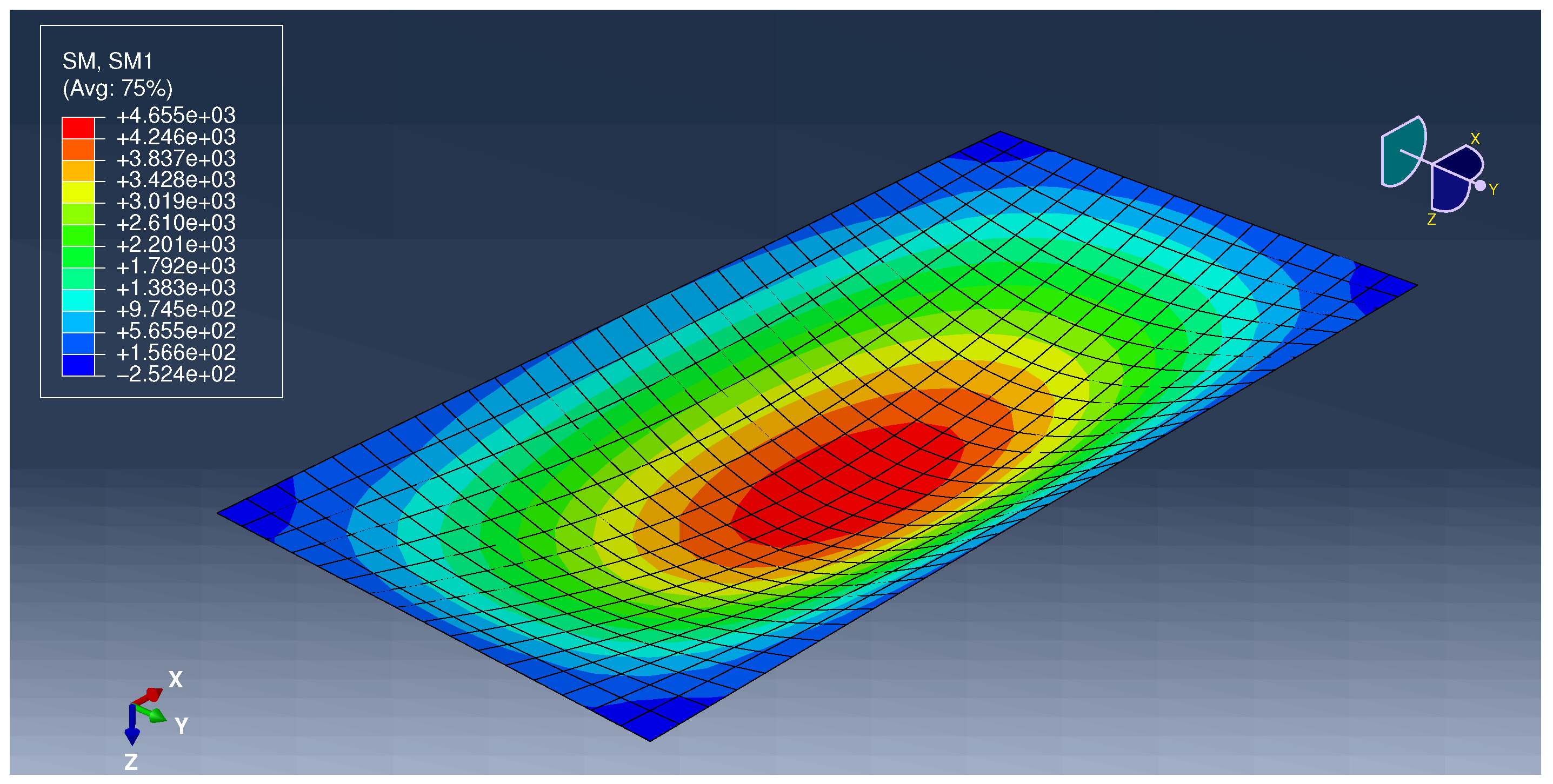
4.2. Rectangular Plate Simply Supported at the Contour

Following boundary conditions must be satisfied (see Figure 12)
w ( x 1 , x 2 ) | x 1 = ± a 1 = 0 ; M 11 ( x 1 , x 2 ) | x 1 = ± a 1 = 0 ; w ( x 1 , x 2 ) | x 2 = ± a 2 = 0 ; M 22 ( x 1 , x 2 ) | x 2 = ± a 2 = 0 .
Three-dimensional plots of deflection of simply supported rectangular plate w and bending moments M 11 , M 22 are given in Figure 13, Figure 14 and Figure 15.
Figure 16, Figure 17 and Figure 18 show cross-sectional plots of deflections and moments.
Extreme values of these magnitudes are collected in Table 3. They exactly coincide with the Timoshenko solution [7]. The maximum values are close to the maximum values obtained in the ABAQUS package (Appendix A.2), but the minimum ones for bending moments do not coincide.
Compliance with boundary conditions at the midpoints of the edges is presented in Table 4. In this example numerical studies have been shown that boundary conditions are satisfied with high accuracy −1 × 10⁻³⁰ for deflection and 1 × 10⁻²⁰ for bending moments.

4.3. Rectangular Plate Clamped at the Contour

Following boundary conditions must be satisfied (see Figure 19)
w ( x 1 , x 2 ) | x 1 = ± a 1 = 0 ; φ 1 ( x 1 , x 2 ) | x 1 = ± a 1 = 0 ; w ( x 1 , x 2 ) | x 2 = ± a 2 = 0 ; φ 2 ( x 1 , x 2 ) | x 2 = ± a 2 = 0 .
Three-dimensional plots of deflection w and bending moments M 11 , M 22 in rectangular plate clamped at the contour are given in Figure 20, Figure 21 and Figure 22.
Figure 23, Figure 24 and Figure 25 show cross-sectional plots of deflections and slopes.
In this example, numerical studies showed that boundary conditions were met with high accuracy − 1 × 10⁻⁸ for deflection and 1 × 10⁻⁷ for slopes. It is seen that symmetry and antisymmetry conditions are performed. The deflection of the center of considered plate is less than previous plate. At the middle cross-section, the bending moment in the center of the plate is smaller than at the edge.
Results of calculations are presented in Table 5. As in previous examples the maximum values of theoretical results are close to the maximum values of results obtained in the ABAQUS package (Appendix A.3), but the minimum ones for bending moments do not coincide.
The numerical results of bending problem of clamped rectangular thin plates presented in [77] are in excellent agreement between the exact numerical-analytical solution obtained by the generalized integral transform technique (GITT) and FEM obtained by the commercial program ABAQUS, but during the analysis, the plates were discretized using sufficiently refined S4R elements − 200 elements in the x direction and 200 × c elements in the y direction. This means that sufficient accuracy was obtained for 40,000 elements, while in the examples presented in this article, the model consists of 512 elements.
Compliance with boundary conditions at the midpoints of the edges is presented in Table 6. Boundary conditions are satisfied exactly.
Figure 26, Figure 27 and Figure 28 illustrate influence of number of approximations on the values of deflection and bending moments M 11 , M 22 in the clamped plate. The results were obtained in section x 2 = 0 of a plate.
Plots are constructed for all approximations from 1 to 5. It is seen that beginning from second approximations ( K = 2 ) they are coincided exactly. This confirms the choice of ( K = 3 ) for calculations.

5. Discussion

Solution of equilibrium equation consists of two parts: general and particular solution which are independent of each other. The general solution identically satisfies differential equation and, in contrast to FEM, satisfies kinematic, static and mixed boundary conditions. The general solution obtained for a rectangular plate is correct for any plate inscribed in a rectangular contour. Particular solution satisfies non-uniform equation of equilibrium using boundary collocation method. It also allows the consideration of plates with arbitrary configurations. Since symmetrical problems are considered, deflections and bending moments are symmetrical functions of variables ( x 1 , x 2 ) but slopes are nonsymmetrical ones.
Advantages of suggested method:
  • Simplicity of structure modeling,
  • Possibility to define static, kinematic and mixed boundary conditions,
  • High accuracy and efficiency of calculation,
  • Meshless approach for solving the problem.
Neither a surface mesh as in FEM nor a boundary mesh as in BEM are required. Introduced nodes are not vertex of finite elements. Surface and edge nodes are generated automatically. Contrary to FEM [78], the presented method is based on continuum model of material. For this reason, operations such as structure discretization and finite element aggregation are unnecessary. Singular plate can be considered to be one global or macro plate element.
Disadvantages of presented method:
  • It cannot be used directly to solve fracture mechanics problems,
  • It is worked for simply connected structures; for each additional contour, it is necessary to introduce the new block of basic functions,
  • It gives good results for regular plates; plates with irregular geometry are solved with less accuracy,
  • Unlike FEM, system matrix is consisted from zero and non-zero blocks.
Table 1, Table 2, Table 3, Table 4, Table 5 and Table 6 contain the minimal and maximal values of static and kinematic magnitudes of the plate obtained by author’s program based on proposed method written in Python programming language, using finite element method in ABAQUS package, and based on the formulae for a simply supported plate according to Navier’s method, included in Timoshenko’s monograph [7].
It is seen that analytical and numerical results of kinematic magnitudes coincide. Maximal values of the bending moments are close but they do not coincide. Twisting moments are differ significantly. Numerical values of bending moments are not zero along the edges of the plate. It follows that static boundary conditions are not met in ABAQUS package.
The reason for this discrepancy is as follows:
  • Presented method is based on Kirchhoff theory of the plates which is deformation theory of zeroth-order where deformations of a cross-section are omitted. Instead generalized shearing force as a sum of shearing forces and derivative of twisting moments is introduced.
  • ABAQUS package is based on Mindlin plate theory which is deformation theory of first-order where deformations of a cross-section are taken into account. Twisting moments and shearing forces are independent ones. It is reason that obtained values of bending and twisting moments are different.
  • Relatively small number of finite elements. The Student Edition of the ABAQUS package is restricted to 1000 nodes.
In analytical approach kinematic and static boundary conditions are performed directly at the separate points at the plate contour. Numerical methods perfectly satisfy kinematic continuity equations and kinematic boundary conditions only at the separate nodes. Equations of equilibrium and static boundary conditions are fulfilled approximately in the whole area of the plate using Principle of Virtual Work. It can be reason that kinematic boundary conditions are satisfied very well but static ones are performed with less accuracy in Finite Element Method.

6. Conclusions

There are many analytical, numerical and analytical-numerical methods to solve thin plates. Most of them are based on the theory of thin plates (see Section 2). Method presented in the paper is one of them. The essence of the method is as follows:
  • to obtain with high accuracy particular solution of equilibrium equations at the separate surface nodes using boundary collocation method,
  • to generate set of the initial points at the coordinate axis and then their distribution at the plate contour,
  • to write boundary conditions at each edge nodes; number of these nodes always corresponds to number of unknown parameter of the model,
  • to solve system of boundary equations,
  • to calculate the desired magnitudes,
  • to prepare the results.
The major findings of this research are summarized in the following:
  • The mathematical model of thin isotropic plates is constructed. Basic shape and force functions are introduced.
  • Within the model equilibrium equations are performed exactly.
  • Expansion of the deflection within the area of the plate is obtained as sum of shape and force functions multiplied by unknown parameters.
  • Displacements, slopes, moments and shearing forces are obtained using method of automatic differentiation. Union of presented relations create mathematical model of the plate.
  • Within constructed model, a method to solving plate of arbitrary geometry have been suggested.
  • All operations are performed automatically with author’s program.
  • Effectiveness of method were illustrated at the examples of rectangular plates with various boundary conditions. Obtained results have been compared with numerical ones computed in ABAQUS package.
  • With help of suggested method three kinds of the rectangular plates, namely: plate with two opposite edges simply supported and the other free; plate simply supported and clamped at the contour were solved. It has been shown that suggested method performs all boundary conditions. Finite element method performs exactly only kinematic ones. Static boundary conditions are performed with less accuracy.
It is shown that chosen direction is actual and important from a practical point of view.

Author Contributions

Conceptualization, M.D; methodology, M.D. and K.R.; software, K.R.; validation, M.D.; writing–original draft preparation, M.D.; writing–review and editing, M.D. and K.R.; visualization, K.R.; supervision, M.D.; project administration, M.D.; All authors have read and agreed to the published version of the manuscript.

Funding

This research received no external funding.

Conflicts of Interest

The authors declare no conflict of interest.

Abbreviations

The following notations are used in this manuscript:
x 1 , x 2 , x 3 Rectangular coordinates
hThickness of a plate
q 0 Intensity of a continuously distributed load
EModulus of elasticity in tension and compression
ν Poisson’s ratio
DFlexural rigidity of a plate
wDeflection of the plate
φ 1 , φ 2 Slopes of the deflection
M 11 , M 22 Bending moments per unit length of sections of a plate perpendicular to x 1 and x 2 axes, respectively
M 12 Twisting moment per unit length of sections of a plate perpendicular to x 1 axis
Q 1 , Q 2 Shearing forces parallel to x 3 axis per unit length of sections of a plate perpendicular to x 1 and x 2 axes, respectively
V 1 , V 2 Generalized shearing forces parallel to x 3 axis per unit length of sections of a plate perpendicular to x 1 and x 2 axes

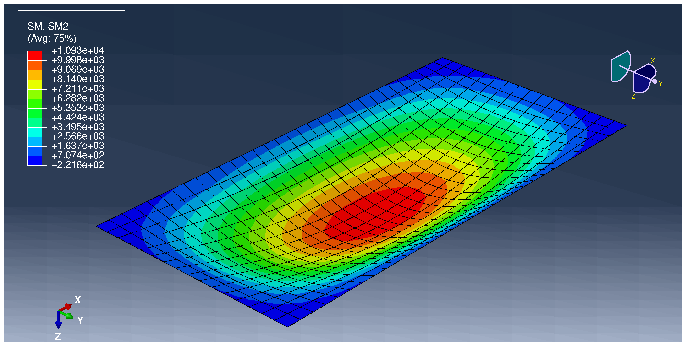
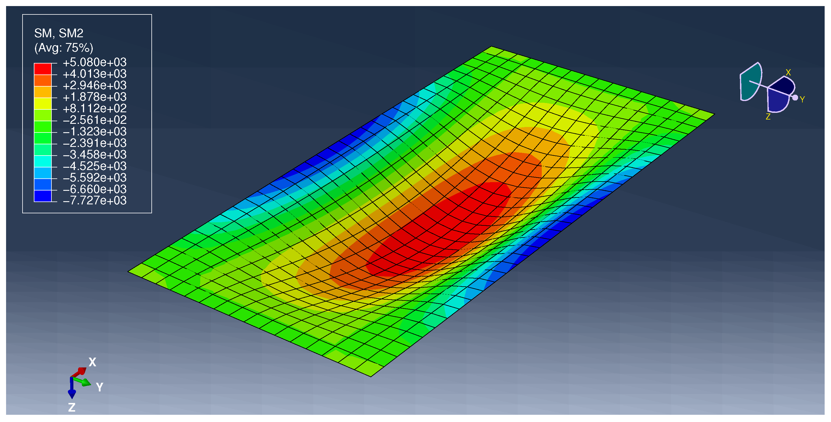
Appendix A. Results from ABAQUS

Results from ABAQUS CAE package are presented below. They correspond to the examples described in this paper.
1
Rectangular plate with two opposite edges simply supported and the other free,
2
Rectangular plate simply supported at the contour,
3
Rectangular plate clamped at the contour.

Appendix A.1. Example 1

Figure A1. The deflection of a rectangular plate with two opposite edges simply supported and the other free solved using FEM.
Applsci 10 05931 g0a1
Figure A2. The bending moment M 11 of a rectangular plate with two opposite edges simply supported and the other free solved using FEM.
Applsci 10 05931 g0a2
Figure A3. The bending moment M 22 of a rectangular plate with two opposite edges simply supported and the other free solved using FEM.
Applsci 10 05931 g0a3

Appendix A.2. Example 2

Figure A4. The deflection of a simply supported rectangular plate solved using FEM.
Applsci 10 05931 g0a4
Figure A5. The bending moment M 11 of a simply supported rectangular plate solved using FEM.
Applsci 10 05931 g0a5
Figure A6. The bending moment M 22 of a simply supported rectangular plate solved using FEM.
Applsci 10 05931 g0a6

Appendix A.3. Example 3

Figure A7. The deflection of a rectangular plate with clamped edges solved using FEM.
Applsci 10 05931 g0a7
Figure A8. The bending moment M 11 of a rectangular plate with clamped edges solved using FEM.
Applsci 10 05931 g0a8
Figure A9. The bending moment M 22 of a rectangular plate with clamped edges solved using FEM.
Applsci 10 05931 g0a9

Appendix B. Listing from Author’S Program

import autograd.numpy as np
from autograd import elementwise_grad as grad
import matplotlib.pyplot as plt
from matplotlib import cm
from matplotlib.ticker import LinearLocator
from mpl_toolkits.mplot3d import Axes3D
# ==========
# Parameters
# ==========
# Number of approximations of the solution
_K = 5
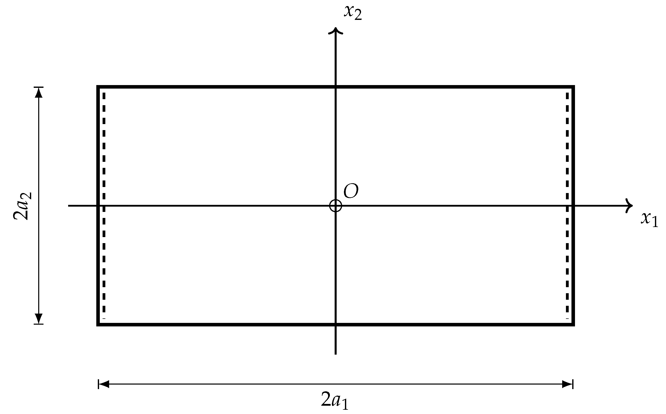
# Dimensions
a_1 = 4.  # m
a_2 = 2.  # m
h = 0.2   # m
# Young’s modulus
E = 3e10  # Pa
# Poisson ratio
nu = 0.2
# Intensity of the load
q_0 = 10_000.00  # N
# Flexural rigidity of a plate
D = (E * h**3) / (12*(1-nu**2))
# ================
# Helper functions
# ================
def a(s):
    if s == 1:
        return a_1
    elif s == 2:
        return a_2
def x(s):
    def wrapper(x_1, x_2):
        if s == 1:
            return x_1
        elif s == 2:
            return x_2
    return wrapper
def gamma(k, s):
    return (k*np.pi) / a(s)
def delta(k, s):
    return ((2*k-1)*np.pi) / (2*a(s))
def kappa(k, p, s):
    if p == 1:
        return gamma(k, s)
    elif p == 2:
        return delta(k, s)
def T(k, p, s):
    def wrapper(x_1, x_2):
        return np.cos(kappa(k, p, s) * x(s)(x_1, x_2))
    return wrapper
def calculate(fs, solution, x_1, x_2):
    coeffs = np.array([f(x_1, x_2) for f in fs])
    return np.einsum(’ijk,i->jk’, coeffs, solution)
def particular_solution(C, f):
    def wrapper(x_1, x_2):
        return C * f(x_1, x_2)
    return wrapper
def final(general_solution, particular_solution):
    result = []
    for f in general_solution:
        result.append(f)
    result.append(particular_solution)
    return result
# ====================================================
# Relations known from theory of thin isotropic plates
# ====================================================
def phi_1(w):
    def wrapper(x_1, x_2):
        return grad(w, 0)(x_1, x_2)
    return wrapper
def phi_2(w):
    def wrapper(x_1, x_2):
        return grad(w, 1)(x_1, x_2)
    return wrapper
def M_11(w):
    def wrapper(x_1, x_2):
        return -D * (grad(grad(w, 0), 0)(x_1, x_2) +
               nu*grad(grad(w, 1), 1)(x_1, x_2))
    return wrapper
def M_22(w):
    def wrapper(x_1, x_2):
        return -D * (grad(grad(w, 1), 1)(x_1, x_2) +
                     nu*grad(grad(w, 0), 0)(x_1, x_2))
    return wrapper
def M_12(w):
    def wrapper(x_1, x_2):
        return -D * (1-nu) * grad(grad(w, 0), 1)(x_1, x_2)
    return wrapper
def Q_1(w):
    def wrapper(x_1, x_2):
        return -D * (grad(grad(grad(w, 0), 0), 0)(x_1, x_2) +
               grad(grad(grad(w, 0), 1), 1)(x_1, x_2))
    return wrapper
def Q_2(w):
    def wrapper(x_1, x_2):
        return -D * (grad(grad(grad(w, 0), 0), 1)(x_1, x_2) +
               grad(grad(grad(w, 1), 1), 1)(x_1, x_2))
    return wrapper
def V_1(w):
    def wrapper(x_1, x_2):
        return -D * (grad(grad(grad(w, 0), 0), 0)(x_1, x_2) +
               (2-nu)*grad(grad(grad(w, 0), 1), 1)(x_1, x_2))
    return wrapper
def V_2(w):
    def wrapper(x_1, x_2):
        return -D * (grad(grad(grad(w, 1), 1), 1)(x_1, x_2) +
               (2-nu)*grad(grad(grad(w, 0), 0), 1)(x_1, x_2))
    return wrapper
# ===============
# Force functions
# ===============
def force_functions(m, n, p, q):
    def wrapper(x_1, x_2):
        return T(m, p, 1)(x_1, x_2) * T(n, q, 2)(x_1, x_2)
    return wrapper
# ===============
# Shape functions
# ===============
# Base functions of the solution
def B(k, p, s, ni):
    def wrapper(x_1, x_2):
        if ni == 1:
            return (np.cosh(kappa(k, p, 3-s) * x(s)(x_1, x_2)))
        elif ni == 2:
            return ((x(s)(x_1, x_2) / a(s)) *
                 (np.sinh(kappa(k, p, 3-s) * x(s)(x_1, x_2))))
    return wrapper
# Shape functions
def W(k, p, s, ni):
    def wrapper(x_1, x_2):
        return B(k, p, s, ni)(x_1, x_2) * T(k, p, 3-s)(x_1, x_2)
    return wrapper
def shape_functions(K):
    result = []
    for k in range(1, K+1):
        for p in range(1, 3):
            for s in range(1, 3):
                for ni in range(1, 3):
                    result.append(W(k, p, s, ni))
    return result
# ===========
# Build model
# ===========
W_g = shape_functions(_K)
W_p = force_functions(1, 1, 2, 2)
# ================
# General solution
# ================
# Calculate derivatives of shape function
U_g = [phi_1(f) for f in W_g]
V_g = [phi_2(f) for f in W_g]
X_g = [M_11(f) for f in W_g]
Y_g = [M_22(f) for f in W_g]
Z_g = [M_12(f) for f in W_g]
H_g = [Q_1(f) for f in W_g]
G_g = [Q_2(f) for f in W_g]
K_g = [V_1(f) for f in W_g]
L_g = [V_2(f) for f in W_g]
# ===================
# Particular solution
# ===================
# Calculate derivatives of force function
U_p = phi_1(W_p)
V_p = phi_2(W_p)
X_p = M_11(W_p)
Y_p = M_22(W_p)
Z_p = M_12(W_p)
H_p = Q_1(W_p)
G_p = Q_2(W_p)
K_p = V_1(W_p)
L_p = V_2(W_p)
C = q_0 / (D*(delta(1, 1)**2 + delta(1, 2)**2)**2)
W_s = particular_solution(C, W_p)
U_s = particular_solution(C, U_p)
V_s = particular_solution(C, V_p)
X_s = particular_solution(C, X_p)
Y_s = particular_solution(C, Y_p)
Z_s = particular_solution(C, Z_p)
H_s = particular_solution(C, H_p)
G_s = particular_solution(C, G_p)
K_s = particular_solution(C, K_p)
L_s = particular_solution(C, L_p)
# ==============
# Final solution
# ==============
W = final(W_g, W_s)
U = final(U_g, U_s)
V = final(V_g, V_s)
X = final(X_g, X_s)
Y = final(Y_g, Y_s)
Z = final(Z_g, Z_s)
H = final(H_g, H_s)
G = final(G_g, G_s)
K = final(K_g, K_s)
L = final(L_g, L_s)
# ===================
# Boundary conditions
# ===================
# Initial points
p_1 = np.linspace(0, a_1, 2*_K)
p_2 = np.linspace(0, a_2, 2*_K)
# Boundary points
b_11 = np.full_like(p_2, a_1)
b_12 = p_2
b_21 = p_1
b_22 = np.full_like(p_1, a_2)
# Shape of blocks
m = len(W)
n = 2*_K
# Initialize matrix blocks
B_1 = np.zeros((m, n))
B_2 = np.zeros((m, n))
B_3 = np.zeros((m, n))
B_4 = np.zeros((m, n))
# Fill matrix blocks with values for boundary conditions 
for i in range(m):
    B_1[i] = W[i](b_11, b_12)
    B_2[i] = U[i](b_11, b_12)
    B_3[i] = W[i](b_21, b_22)
    B_4[i] = V[i](b_21, b_22)
# ============
# Solve system
# ============
# Augmented matrix
M = np.hstack((B_1, B_2, B_3, B_4))
M = M.T
# Coefficient matrix
A = M[:, :-1]
# Column vector of constant terms
b = M[:, -1]
# Solve a linear matrix equation
R = np.linalg.solve(A, -b)
R = np.append(R, 1)
# ==========================
# Calculate and plot results
# ==========================
# Prepare points for calculating the values in them
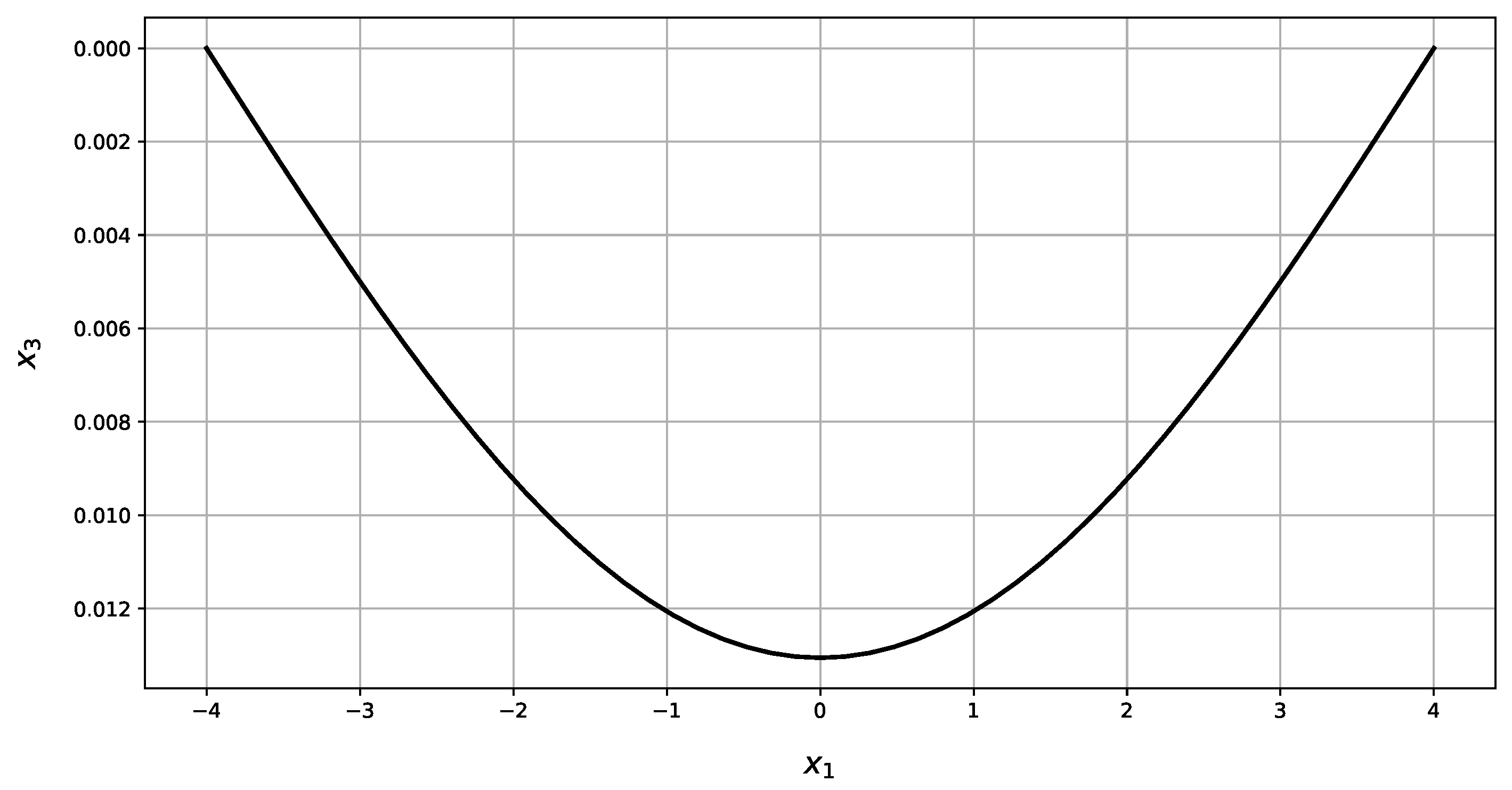
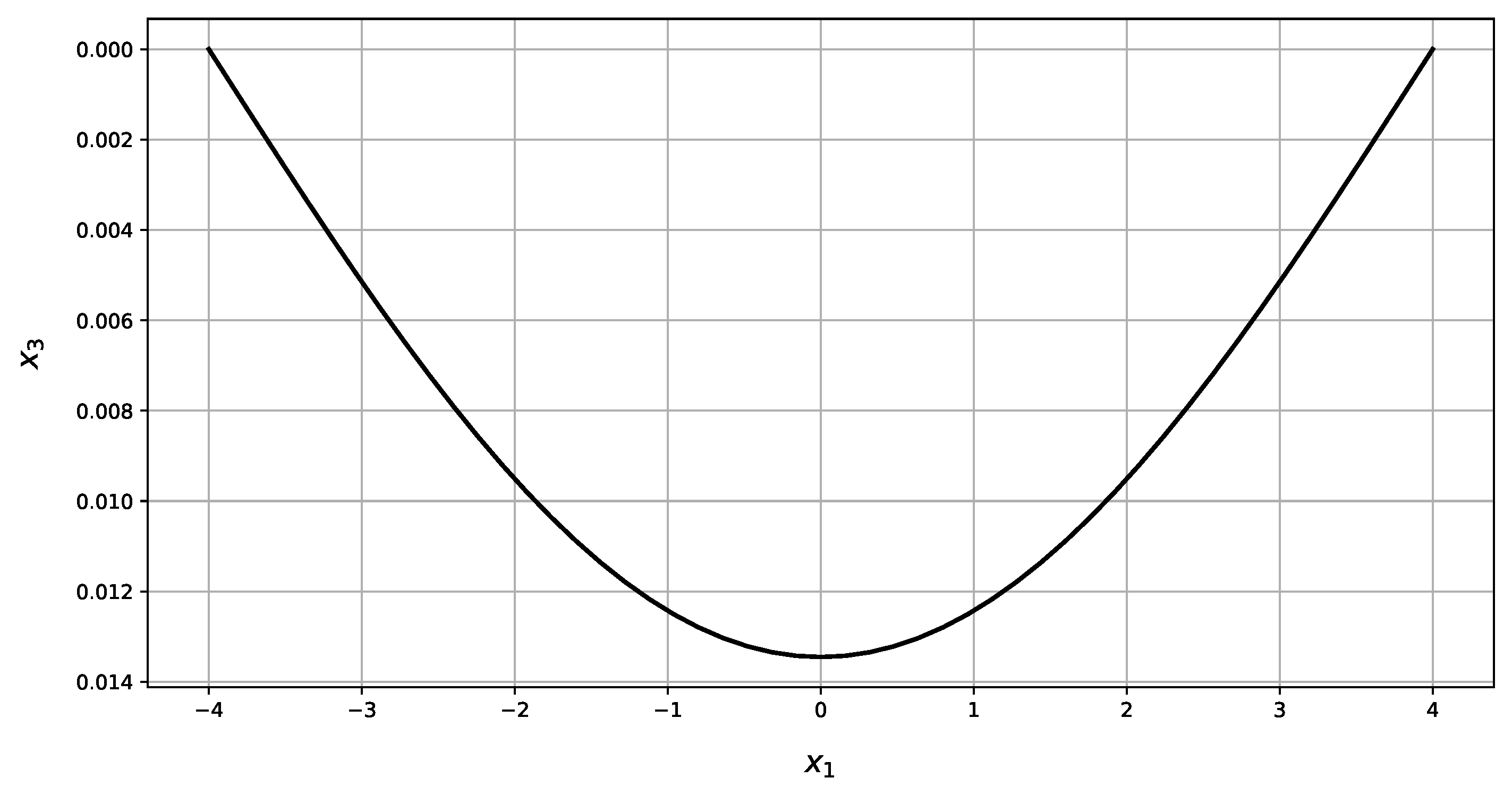
x_1 = np.linspace(-a_1, a_1, num=51)
x_2 = np.linspace(-a_2, a_2, num=51)
X_1, X_2 = np.meshgrid(x_1, x_2)
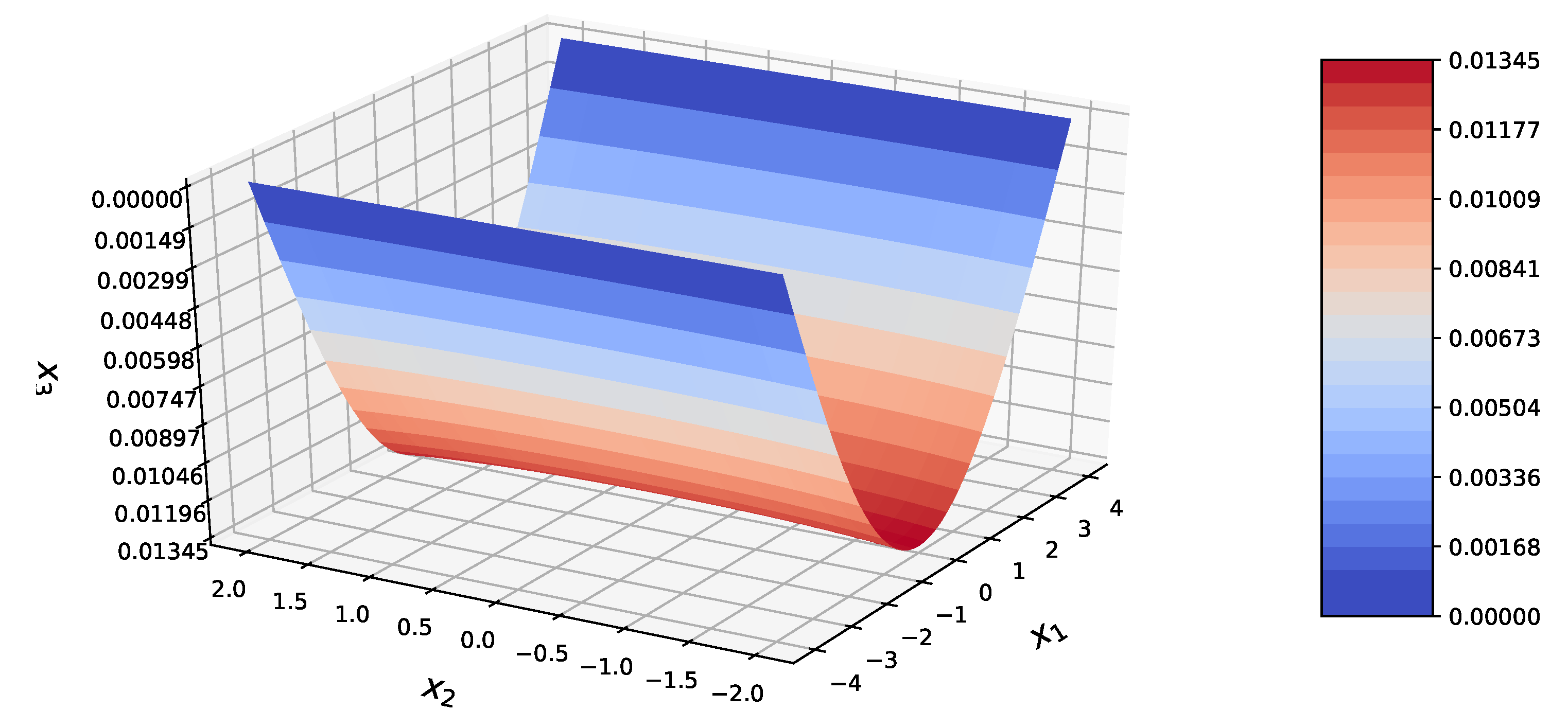
for f in [W, U, V, X, Y, Z, H, G, K, L]:
    X_3 = calculate(f, R, X_1, X_2)
    fig = plt.figure()
    ax = fig.gca(projection=’3d’)
    ax.set_xlabel(’$x_1$’)
    ax.set_ylabel(’$x_2$’)
    ax.set_zlabel(’$x_3$’)
    surf = ax.plot_surface(X_1, X_2, X_3,
                      cmap=cm.coolwarm,
                      linewidth=0,
                      antialiased=True)
    ax.zaxis.set_major_locator(LinearLocator(10))
    ax.set_zlim(ax.get_zlim()[::-1])
    boundaries = np.linspace(np.min(X_3), np.max(X_3), 25)
    fig.colorbar(surf,
              shrink=0.75,
              aspect=5,
              boundaries=boundaries)
    plt.show()
--------------------------------------------------------------------------------

References

  1. Reddy, J. Theory of Elastic Plates and Shells, 2nd ed.; CRC Press Taylor & Francis Group: London, UK; New York, NY, USA, 2010. [Google Scholar]
  2. Szilard, R. Theories and Applications of Plate Analysis. Classical, Numerical and Engineering Methods. Appl. Mech. Rev. 2004, 57, B32–B33. [Google Scholar] [CrossRef]
  3. Dolbow, J.; Moës, N.; Belytschko, T. Modeling fracture in Mindlin–Reissner plates with the extended finite element method. Int. J. Solids Struct. 2000, 37, 7161–7183. [Google Scholar] [CrossRef]
  4. Reddy, J. Third-Order Theory of Laminated Composite Plates and Shells. In Mechanics of Laminated Composite Plates and Shells; CRC Press: Boca Raton, IL, USA, 2003; p. 671. [Google Scholar]
  5. Wang, C.; Reddy, J.; Lee, K. An Overview of Plate Theories. In Shear Deformable Beams and Plates: Relationships with Classical Solutions; Elsevier Science Ltd.: Amsterdam, The Netherlands, 2000; p. 3. [Google Scholar]
  6. Rakowski, G. Sprężystość. Problemy i RozwiąZania. Metody Analityczne i Numeryczne; Wydawnictwo Politechniki Świętokrzyskiej: Kielce, Poland, 2001. [Google Scholar]
  7. Timoshenko, S.; Woinowsky-Krieger, S. Simply supported rectangular plates. In Theory of pLates and Shells; McGraw-Hill Book Company, Inc.: New York, NY, USA, 1959; pp. 105–108. [Google Scholar]
  8. Timoshenko, S.P. Kurs Teorii Uprugosti; Naukova Dumka: Kiev, Ukraine, 1972; pp. 320–364. [Google Scholar]
  9. Grzymkowski, R.; Kapusta, A.; Nowak, I.; Słota, D. Metody Numeryczne. Zagadnienia Brzegowe; WPKJS: Gliwice, Poland, 2003. [Google Scholar]
  10. Skibicki, D.; Nowicki, K. Metody Numeryczne w Budowie Maszyn; Wydawnictwa Uczelniane Akademii Techniczno-Rolniczej w Bydgoszczy: Bydgoszcz, Poland, 2006. [Google Scholar]
  11. Wilson, E. Special numerical and computer techniques for the analysis of finite element systems. In U.S.–Germany Symposium on Finite Elements Methods; MIT: Cambridge, MA, USA, 1976. [Google Scholar]
  12. Kleiber, M. Mechanika Techniczna. Komputerowe Metody Mechaniki Ciał StałYch; PWN: Warszawa, Poland, 1995. [Google Scholar]
  13. Qin, Q. The Trefftz Finite and Boundary Element Method; WIT Press: Southampton, Boston, IL, USA, 2000. [Google Scholar]
  14. Zienkiewicz, O.; Taylor, R. The Finite Element Method, 5th ed.; Butterworth Heinemann: Oxford, UK, 2000; Volume 2. [Google Scholar]
  15. Sikora, J. Numeryczne Metody Rozwiązywania Zagadnień Brzegowych. Podstawy Metody Elementów Skończonych i Metody Elementów Brzegowych; Politechnika Lubelska: Lublin, Poland, 2011. [Google Scholar]
  16. Fadhil, S.; El-Zafrany, A. Boundary element analysis of thick Reissner plates on two-parameter foundation. Int. J. Solids Struct. 1994, 31, 2901–2917. [Google Scholar] [CrossRef]
  17. Brebbia, C. The Boundary Element Method for Engineers; Pentech Press: London, UK, 1978. [Google Scholar]
  18. Myślecki, K. Metoda Elementów Brzegowych w Statyce Dźwigarów Powierzchniowych; Oficyna Wydawnicza Politechniki Wrocławskiej: Wrocław, Poland, 2004. [Google Scholar]
  19. Baydin, A.G.; Pearlmutter, B.A.; Radul, A.A. Automatic differentiation in machine learning: A survey. J. Mach. Learn. Res. 2017, 18, 5595–5637. [Google Scholar]
  20. Bradbury, J.; Frostig, R.; Hawkins, P.; Johnson, M.J.; Leary, C.; Maclaurin, D.; Wanderman-Milne, S. JAX: Composable Transformations of Python+NumPy Programs. 2018. Available online: https://github.com/google/jax (accessed on 25 August 2020).
  21. Woźniak, C. Mechanika Sprężystych Płyt i Powłok; PWN: Warszawa, Poland, 2001. [Google Scholar]
  22. Nwoji, C.; Mama, B.; Ike, C.; Onah, H. Galerkin-Vlasov Method for the Flexural Analysis of Rectangular Kirchhoff Plates with Clamped and Simply Supported Edges. Iosr J. Mech. Civ. Eng. 2017, 14, 61–74. [Google Scholar] [CrossRef]
  23. Reddy, J. Energy Principles and Variational Methods in Applied Mechanics, 3rd ed.; John Wiley & Sons, Inc.: New York, NY, USA, 2017. [Google Scholar]
  24. Navier, C.L.M.H. Extrait des Recherches Sur La Flexion Des Plans Elastiques; Bulletin des Sciences, par la Société Philomatique: Paris, France, 1823; pp. 92–102. [Google Scholar]
  25. Lévy, M. Sur l’équilibre élastique d’une plaque rectangulaire. Comptes Rendus L’AcadéMie Des Sci. Paris 1899, 129, 535–539. [Google Scholar]
  26. Krjukov, N. Raschet kosougol’nyh i trapecoidal’nyh plastin s pomoshh’ju splajn funkcij. Prikl. Meh. 1998, 23, 77–81. [Google Scholar]
  27. Alberg, D.; Nilson, J.; Ullli, D. Teorija splajnov i ee prilozhenie. 1972. Available online: http://libarch.nmu.org.ua/handle/GenofondUA/81626 (accessed on 25 August 2020).
  28. Songbai, C.; Lasbeng, W. Collocation method for bending problem of cantilevered plates subjected to unsymmetrical loads. Hunan Univ. Natur. Sci. 1996, 23, 126–128. [Google Scholar]
  29. Dong, C.; Lo, S.; Cheung, Y.; Lee, K. Anisotropic thin plate bending problems by Trefftz boundary collocation method. Eng. Anal. Bound. Elem. 2004, 28, 1017–1024. [Google Scholar] [CrossRef]
  30. Reddy, J. An Introduction to the Finite Element Method, 3rd ed.; McGraw-Hill: New York, NY, USA, 2006. [Google Scholar]
  31. Rakowski, G.; Kasperczyk, Z. Metoda Elementów Skończonych w Mechanice Konstrukcji; Oficyna Wydawnicza Politechniki Warszawskiej: Warszawa, Poland, 2005. [Google Scholar]
  32. The Finite Element Method: Its Basis and Fundamentals, 7th ed.; Zienkiewicz, O.; Taylor, R.; Zhu, J. (Eds.) Butterworth-Heinemann: Oxford, UK, 2013. [Google Scholar] [CrossRef]
  33. The Finite Element Method for Solid and Structural Mechanics, 7th ed.; Zienkiewicz, O.; Taylor, R.; Fox, D. (Eds.) Butterworth-Heinemann: Oxford, UK, 2014. [Google Scholar] [CrossRef]
  34. Bathe, K.J.; Dvorkin, E.N. A four-node plate bending element based on Mindlin/Reissner plate theory and a mixed interpolation. Int. J. Numer. Methods Eng. 1985, 21, 367–383. [Google Scholar] [CrossRef]
  35. Podhorecki, A. Metoda elementów czasoprzestrzennych w zastosowaniu do rozwiązywania zagadnień początkowo-brzegowych. In Zeszyty Naukowe; Akademia Techniczno-Rolnicza: Bydgoszcz, Poland, 2004; Volume 54. [Google Scholar]
  36. Zhuang, M.; Miao, C. Analysis for Irregular Thin Plate Bending Problems on Winkler Foundation by Regular Domain Collocation Method. Math. Probl. Eng. 2018, 2018, 7476954. [Google Scholar] [CrossRef] [Green Version]
  37. Jiang, W.; Bao, G.; Robert, J. Finite element modeling of stiffened and unstiffened orthotropic plates. Comput. Struct. 1997, 63, 105–117. [Google Scholar] [CrossRef]
  38. Qu, Z.Q. Model Order Reduction Techniques with Applications in Finite Element Analysis; Springer: London, UK, 2004. [Google Scholar]
  39. Shen, P.; He, P. Bending analysis of rectangular moderately thick plates using spline finite element method. Comput. Struct. 1995, 54, 1023–1029. [Google Scholar] [CrossRef]
  40. Dieringer, R.; Hebel, J.; Becker, W. The scaled boundary finite element method for plate bending problems. In Proceedings of the 19th International Conference on Computer Methods in Mechanics 2011, Warsaw, Poland, 9–12 May 2011. [Google Scholar]
  41. Belyaev, V.; Shapeev, V. Solving the biharmonic equation in irregular domains by the least squares collocation method. AIP Conf. Proc. 2018, 2027, 030094. [Google Scholar] [CrossRef]
  42. Li, R.; Zhong, Y.; Tian, B. On new symplectic superposition method for exact bending solutions of rectangular cantilever thin plates. Mech. Res. Commun. Mech. Res. Commun. 2011, 38, 111–116. [Google Scholar] [CrossRef]
  43. Alansari, M.; Afzal, M. Regular and Irregular Plate Deflection Analysis using Matrix Method. IOSR J. Mech. Civ. Eng.-(IOSR-JMCE) 2019, 16, 24–40. [Google Scholar] [CrossRef]
  44. Armando Duarte, C.; Kim, D.J.; Babuška, I. A Global-Local Approach for the Construction of Enrichment Functions for the Generalized FEM and Its Application to Three-Dimensional Cracks. In Advances in Meshfree Techniques; Leitão, V.M.A., Alves, C.J.S., Armando Duarte, C., Eds.; Springer: Dordrecht, The Netherlands, 2007; pp. 1–26. [Google Scholar]
  45. Duarte, C.; Kim, D.J. Analysis and applications of a generalized finite element method with global–local enrichment functions. Comput. Methods Appl. Mech. Eng. 2008, 197, 487–504. [Google Scholar] [CrossRef]
  46. Kim, D.J.; Duarte, C.A.; Pereira, J.P. Analysis of Interacting Cracks Using the Generalized Finite Element Method With Global-Local Enrichment Functions. J. Appl. Mech. 2008, 75. [Google Scholar] [CrossRef]
  47. Gupta, V.; Kim, D.J.; Duarte, C.A. Analysis and improvements of global–local enrichments for the Generalized Finite Element Method. Comput. Methods Appl. Mech. Eng. 2012, 245–246, 47–62. [Google Scholar] [CrossRef]
  48. Malekan, M.; Barros, F.A.c.B.; Pitangueira, R.L.S.; Alves, P.D. An Object-Oriented Class Organization for Global-Local Generalized Finite Element Method. Lat. Am. J. Solids Struct. 2016, 13, 2529–2551. [Google Scholar] [CrossRef] [Green Version]
  49. Malekan, M.; Barros, F.; Pitangueira, R.; Alves, P.; Penna, S. A computational framework for a two-scale generalized/extended finite element method: Generic imposition of boundary conditions. Eng. Comput. 2016, 34. [Google Scholar] [CrossRef] [Green Version]
  50. Malekan, M.; Barros, F.B. Well-conditioning global–local analysis using stable generalized/extended finite element method for linear elastic fracture mechanics. Comput. Mech. 2016, 58, 819–831. [Google Scholar] [CrossRef]
  51. Malekan, M.; Barros, F.B.; Pitangueira, R.L. Fracture analysis in plane structures with the two-scale G/XFEM method. Int. J. Solids Struct. 2018, 155, 65–80. [Google Scholar] [CrossRef]
  52. Baiz, P.; Natarajan, S.; Bordas, S.; Kerfriden, P.; Rabczuk, T. Linear buckling analysis of cracked plates by SFEM and XFEM. J. Mech. Mater. Struct. 2011, 6, 1213–1238. [Google Scholar] [CrossRef] [Green Version]
  53. Nasirmanesh, A.; Mohammadi, S. XFEM buckling analysis of cracked composite plates. Compos. Struct. 2015, 131, 333–343. [Google Scholar] [CrossRef]
  54. Perumal, L.; Tso, C.; Leng, L.T. Analysis of thin plates with holes by using exact geometrical representation within XFEM. J. Adv. Res. 2016, 7, 445–452. [Google Scholar] [CrossRef] [PubMed] [Green Version]
  55. Benvenuti, E. An effective XFEM with equivalent eigenstrain for stress intensity factors of homogeneous plates. Comput. Methods Appl. Mech. Eng. 2017, 321, 427–454. [Google Scholar] [CrossRef]
  56. Donning, B.M.; Liu, W.K. Meshless methods for shear-deformable beams and plates. Comput. Methods Appl. Mech. Eng. 1998, 152, 47–71. [Google Scholar] [CrossRef]
  57. Shao, W.; Wu, X. Chebyshev tau meshless method based on the highest derivative for solving a class of two-dimensional parabolic problems. Wit Trans. Model. Simul. 2013. [Google Scholar] [CrossRef] [Green Version]
  58. Liu, N.; Jeffers, A.E. A geometrically exact isogeometric Kirchhoff plate: Feature-preserving automatic meshing and C1 rational triangular Bézier spline discretizations. Int. J. Numer. Methods Eng. 2018, 115, 395–409. [Google Scholar] [CrossRef]
  59. Liu, N.; Ren, X.; Lua, J. An isogeometric continuum shell element for modeling the nonlinear response of functionally graded material structures. Compos. Struct. 2020, 237, 111893. [Google Scholar] [CrossRef]
  60. Batista, M. Uniformly Loaded Rectangular Thin Plates with Symmetrical Boundary Conditions. arXiv 2010, arXiv:1001.3016. [Google Scholar]
  61. Batista, M. New analytical solution for bending problem of uniformly loaded rectangular plate supported on corner points. IES J. Part Civ. Struct. Eng. 2010, 3, 75–84. [Google Scholar] [CrossRef]
  62. Li, R.; Zhong, Y.; Tian, B.; Du, J. Exact bending solutions of orthotropic rectangular cantilever thin plates subjected to arbitrary loads. Int. Appl. Mech. 2011, 47, 107–119. [Google Scholar] [CrossRef] [Green Version]
  63. Ike, C.C. Flexural analysis of rectangular kirchhoff plate on winkler foundation using galerkin-vlasov variational method. Math. Model. Eng. Probl. 2018, 5, 83–92. [Google Scholar] [CrossRef]
  64. Hwu, C.; Huang, S.T.; Li, C.C. Boundary-based finite element method for two-dimensional anisotropic elastic solids with multiple holes and cracks. Eng. Anal. Bound. Elem. 2017, 79, 13–22. [Google Scholar] [CrossRef]
  65. Guminiak, M. Zastosowanie metody elementów brzegowych w analizie statyki płyt cienkich. Zesz. Nauk. Politech. Śląskiej 2002, 95, 223–232. [Google Scholar]
  66. Tanaka, M.; Bercin, A. A boundary element method applied to the elastic bending problem of stiffened plates. Bound. Elem. Method XIX 1997, 19, 203–212. [Google Scholar]
  67. Delyavskyy, M.; Opanasovych, V.; Bilash, O. Bending by Concentrated Force of a Cantilever Strip Having a Through-thickness Crack Perpendicular to Its Axis. Appl. Sci. 2020, 10, 2037. [Google Scholar] [CrossRef] [Green Version]
  68. Delyavskyy, M.; Rosiński, K. Analiza statyczna złożonych konstrukcji płytowych w ujęciu makroelementowym. Czas. Inżynierii Lądowej Środowiska i Archit. 2016. [Google Scholar] [CrossRef] [Green Version]
  69. Delyavskyy, M.; Rosiński, K. Solution of non-rectangular plates with macroelement method. AIP Conf. Proc. 2017, 1822, 020005. [Google Scholar] [CrossRef]
  70. Delyavs’kyi, M.; Zdolbits’ka, N.; Onyshko, L.; Zdolbits’kyi, A. Determination of the Stress-Strain State in Thin Orthotropic Plates on Winkler’s Elastic Foundations. Mater. Sci. 2015, 50. [Google Scholar] [CrossRef]
  71. Delyavskyy, M.; Rosiński, K.; Zdolbicka, N.; Bilash, O. Macroelement analysis of thin orthotropic polygonal plate resting on the elastic Winkler’s foundation. AIP Conf. Proc. 2019, 2077, 020014. [Google Scholar] [CrossRef]
  72. Delyavskyy, M.; Rosiński, K. Analysis of Thin Rectangular Plate Connected With Space Truss; MOSTY Tradycja i Nowoczesność; Wydawnictwa Uczelniane Uniwersytetu Technologiczno-Przyrodniczego w Bydgoszczy: Bydgoszcz, Poland, 2019. [Google Scholar]
  73. Delyavskyy, M.; Rosiński, K. Rozwiązanie Konstrukcji Inżynierskich w Ujęciu Makroelementowym; Wybrane zagadnienia konstrukcji i materiałów budowlanych oraz geotechniki. Wydawnictwa Uczelniane Uniwersytetu Technologiczno-Przyrodniczego w Bydgoszczy: Bydgoszcz, Poland, 2015. [Google Scholar]
  74. Barthelemy, J.F.M.; Hall, L.E. Automatic differentiation as a tool in engineering design. Struct. Optim. 1995, 9, 76–82. [Google Scholar] [CrossRef] [Green Version]
  75. Lim, C.W.; Yao, W.A.; Cui, S. Benchmark symplectic solutions for bending of corner-supported rectangular thin plates. IES J. Part Civ. Struct. Eng. 2008, 1, 106–115. [Google Scholar] [CrossRef]
  76. Li, R.; Wang, B.; Li, G. Benchmark bending solutions of rectangular thin plates point-supported at two adjacent corners. Appl. Math. Lett. 2015, 40, 53–58. [Google Scholar] [CrossRef]
  77. An, C.; Gu, J.; Su, J. Exact solution of bending problem of clamped orthotropic rectangular thin plates. J. Braz. Soc. Mech. Sci. Eng. 2015, 38. [Google Scholar] [CrossRef]
  78. Pavlou, D. Main Disadvantages of Finite Element Method. In Essentials of the Finite Element Method For Mechanical and Structural Engineers; Elsevier Inc.: Amsterdam, The Netherlands, 2015. [Google Scholar]
Figure 1. Scheme of the symmetrical plate.
Applsci 10 05931 g001
Figure 2. Distribution of current nodes at the contour of rectangular plate.
Applsci 10 05931 g002
Figure 3. Rectangular plate with two opposite edges simply supported and the other free.
Applsci 10 05931 g003
Figure 4. Three-dimensional plot of the deflection of a rectangular plate with two opposite edges simply supported and the other free.
Applsci 10 05931 g004
Figure 5. Three-dimensional plot of the bending moment M 11 of a rectangular plate with two opposite edges simply supported and the other free.
Applsci 10 05931 g005
Figure 6. Three-dimensional plot of the bending moment M 22 of a rectangular plate with two opposite edges simply supported and the other free.
Applsci 10 05931 g006
Figure 7. The deflection in section x 2 = 0 of a rectangular plate with two opposite edges simply supported and the other free.
Applsci 10 05931 g007
Figure 8. The deflection in section x 2 = 2 of a rectangular plate with two opposite edges simply supported and the other free.
Applsci 10 05931 g008
Figure 9. The deflection in section x 1 = 0 of a rectangular plate with two opposite edges simply supported and the other free.
Applsci 10 05931 g009
Figure 10. The bending moments M 11 in section x 1 = 0 of a rectangular plate with two opposite edges simply supported and the other free.
Applsci 10 05931 g010
Figure 11. The bending moments M 22 in section x 1 = 0 of a rectangular plate with two opposite edges simply supported and the other free.
Applsci 10 05931 g011
Figure 12. Simply supported rectangular plate.
Applsci 10 05931 g012
Figure 13. Three-dimensional plot of the deflection of simply supported rectangular plate.
Applsci 10 05931 g013
Figure 14. Three-dimensional plot of the bending moment M 11 of simply supported rectangular plate.
Applsci 10 05931 g014
Figure 15. Three-dimensional plot of the bending moment M 22 of simply supported rectangular plate.
Applsci 10 05931 g015
Figure 16. The deflection in section x 2 = 0 of a simply supported rectangular plate.
Applsci 10 05931 g016
Figure 17. The bending moments M 11 in section x 2 = 0 of a simply supported rectangular plate.
Applsci 10 05931 g017
Figure 18. The bending moments M 22 in section x 1 = 0 of a simply supported rectangular plate.
Applsci 10 05931 g018
Figure 19. Rectangular plate clamped at the contour.
Applsci 10 05931 g019
Figure 20. Three-dimensional plot of the deflection of a rectangular plate with clamped edges.
Applsci 10 05931 g020
Figure 21. Three-dimensional plot of the bending moment M 11 of a rectangular plate with clamped edges.
Applsci 10 05931 g021
Figure 22. Three-dimensional plot of the bending moment M 22 of a rectangular plate with clamped edges.
Applsci 10 05931 g022
Figure 23. The deflection in section x 2 = 0 of a rectangular plate with clamped edges.
Applsci 10 05931 g023
Figure 24. The slope φ 1 in section x 2 = 0 of a rectangular plate with clamped edges.
Applsci 10 05931 g024
Figure 25. The slope φ 2 in section x 1 = 0 of a rectangular plate with clamped edges.
Applsci 10 05931 g025
Figure 26. The deflection in section x 2 = 0 of a rectangular plate with clamped edges for different number of approximations.
Applsci 10 05931 g026
Figure 27. The bending moments M 11 in section x 2 = 0 of a rectangular plate with clamped edges for different number of approximations.
Applsci 10 05931 g027
Figure 28. The bending moments M 22 in section x 2 = 0 of a rectangular plate with clamped edges for different number of approximations.
Applsci 10 05931 g028
Table 1. Minimal and maximal values of kinematic and static magnitudes with their relative error (RE).
Present MethodAbaqusRE
MagnitudeUnitMinMaxMinMaxMinMax
w m 00.01300.0130%0%
M 11 N m 041,490.63194441,3100.44%
M 22 N m 05516.33−78.0253113.87%
M 12 N m −3263.793263.79−2402240235.88%35.88%
Q 1 N −15,343.3615,343.36
Q 2 N −3229.423229.42
V 1 N −14,440.9514,440.95
V 2 N −2677.452677.45
φ 1 rad −0.0050.005−0.0050.0050%0%
φ 2 rad −0.00050.0005−0.00050.00050%0%
Table 2. Compliance with boundary conditions at the midpoints of the edges.
MagnitudeEdgeUnitPresent MethodAbaqus
wSimply supported m 00
M 11 Simply supported N m 01966.02
M 22 Free N m 0288.97
V 2 Free N 0
Table 3. Minimal and maximal values of magnitudes with their relational error (RE).
Present MethodTimoshenkoAbaqusRE
MagnitudeUnitMinMaxMinMaxMinMaxMinMax
w m 0.000.00080.000.00080.000.00080%0%
M 11 N m 0.004668.880.004668.88−252.446550.30%
M 22 N m 0.0010,894.050.0010,894.05−221.610,930−0.33%
M 12 N m −4150.124150.12−4150.124150.12−404140412.70%
Q 1 N −5092.965092.96−5092.965092.96
Q 2 N −10,185.9210,185.92−10,185.9210,185.92
V 1 N −8352.458352.45−8352.458352.45
V 2 N −11,815.6611,815.66−11,815.6611,815.66
φ 1 rad −0.00030.0003−0.00030.0003−0.00030.00030%0%
φ 2 rad −0.00060.0006−0.00060.0006−0.00060.00060%0%
Table 4. Compliance with boundary conditions at the midpoints of the edges.
MagnitudeEdgeUnitPresent MethodTimoshenkoAbaqus
wSimply supported 1 m 000
M 11 Simply supported 1 N m 00416.46
wSimply supported 2 m 000
M 22 Simply supported 2 N m 001170.5
Table 5. Minimal and maximal values of magnitudes with their relational error (RE).
Present MethodAbaqusRE
MagnitudeUnitMinMaxMinMaxMinMax
w m 0.000.00020.000.00020%0%
M 11 N m −4174.731909.82−3326187725.52%1.75%
M 22 N m −9305.645180.73−7727508020.43%1.98%
M 12 N m −1190.871190.87−112011206.33%6.33%
Q 1 N −6806.216806.21
Q 2 N 12 , 667.36 12 , 667.36
V 1 N −7268.187268.18
V 2 N 12 , 667.93 12 , 667.93
φ 1 rad 0.000.000.000.000%0%
φ 2 rad −0.00020.0002−0.00020.00020%0%
Table 6. Compliance with boundary conditions at the midpoints of the edges.
MagnitudeEdgeUnitPresent MethodAbaqus
wClamped 1 m 00
φ 1 Clamped 1 rad 00
wClamped 2 m 00
φ 2 Clamped 2 rad 00

