Vibration Parameters Estimation by Blade Tip-Timing in Mistuned Bladed Disks in Presence of Close Resonances

Abstract

The present paper is focused on the post processing of the data coming from the Blade Tip-Timing (BTT) sensors in the case where two very close peaks are present in the frequency response of the vibrating system. This type of dynamic response with two very close peaks can occur quite often in bladed disks. It is related to the fact that the bladed disk is not perfectly cyclic symmetric and the so called “mistuning” is present. A method based on the fitting of the BTT sensors data by means of a 2 degrees of freedom (2DOF) dynamic model is proposed. Nonlinear least square optimization technique is employed for identification of the vibration characteristics. A numerical test case based on a lump parameter model of a bladed disk assembly is used to simulate different response curves and the corresponding sensors signals. The Frequency Response Function (FRF) constructed at the resonance region is compared with the traditional Sine fitting results, the resonance frequencies and damping values estimated by the fitting procedure are also reported. Accurate predictions are achieved and the results demonstrate the considerable capacity of the 2DOF method to be used as a standalone or as a complement to the standard Sine fitting method.

1. Introduction

Turbomachinery blades can reach critical vibration amplitude during operating conditions. Undesirable vibrations occur when the blade passes through a resonance. Resonances in the blades can be excited by the fluctuations downstream and upstream of the flow path inducing alternating aerodynamic loadings, which are the major sources of blade excitations. In resonance conditions, blades vibrations can be excessively increased with the risk of incurring a High Cycle Fatigue failure. Measuring the vibration parameters of the rotating blades is therefore of great interest to engineers at two different levels:

-

in the laboratory during the engine test phase, to obtain the natural frequencies and the damping of the blade and blisk (integrally bladed rotor [1]) in order to have experimental parameters to update the numerical models;

-

in operation for the control of vibrations and for monitoring the health of the engine.

Vibration measurements of rotating blades are traditionally performed by means of strain gauge technology [2]. This method has been developed over time and successfully employed for an extensive range of engineering applications. Currently, it is considered as a well-established technology with the most accurate and reliable results. However the limits of the use of strain gauges are that:

• they only measure the deformation of the blades on which they are glued, they must therefore be glued on all the blades to control them all;
• they are connected to telemetry/slip ring; this might require important changes to rotating and stationary parts and implies integration of instrumentation hardware, in order to get accurate vibration response with the best Signal-to-Noise Ratio (SNR), these modifications are costly and time consuming;
• the adaptations required by the strain gauge installation could lead to constraints for some other turbomachine parameters (for instance, the aerodynamic ones).

To minimize the adverse effects of the strain gauges and in response to the high demands for having a non-intrusive blade vibration measurement system, non-contact measurement technology has been developed. Blade Tip-Timing (BTT) is a non-contact measurement method that has attracted considerable attention in previous decades among turbomachinery specialists. This method is still under development in order to enhance its capabilities to become the reference technique for measurement of vibrations in rotating blade assemblies. The main manufacturers of turbo engines have invested in recent years in improving the vibration measurement system based on BTT technology [3]. The main advantage of the BTT method is the simultaneous monitoring of all blades as well as non-intrusive aspects, easy set-up and data transmission. Its major shortcoming is the under-sampling of the signal related to the rotational speed of the rotating disk under study. The research works on BTT in the last years are about the main areas of the sensor development [4,5], signal processing, vibration parameters identification and the application of this method for condition monitoring [6,7,8]. The present paper is focused on the post-processing of the BTT data to estimate the main vibration parameters even in the case of very close or overlapped resonance peaks. One of the earliest works in this area is the well-known single parameter method introduced by Zablotskiy and Korostelev [9] in 1970. This method was proposed based on a single degree of freedom (SDOF or 1DOF) vibrating system, the maximum vibration amplitude is obtained by deriving the peak to peak values of the deflection signal. Next, Heath and Imregun [10] proposed an amendment for the single parameter method by considering the effects of blade vibration on the computation of the arrival time. Then, in 2000, Heath [11] presented a new analysis technique called two-parameter plot method for identifying synchronous resonance vibration by using two tip-timing sensors. Schlagwein and Schaber [12] developed a multi-degrees-of-freedom method for obtaining the vibration parameters of mistuned rotating blades. The method was implemented on simulated and measured data and a good match with strain gauge measurements was reported. Recently, Rigosi et al. [13] suggested a revision for two-parameter plot method. They actually proposed an alternative procedure to determine the Engine Order (EO) and the vibration amplitude and they compared their results with the results obtained by the strain gauges measurements.

The methods introduced so far are recognized as indirect methods, they require measurements data from one or two sensors. All samples of the deflection signal recorded by the sensors over the entire resonance region are used for the vibration parameters identification. In addition, there exist other types of analysis methods called direct methods in which at least four probes are employed for analyzing tip timing data. Least-squares Sine fitting algorithm presented by Heath [14] is the most common direct method used for parameters identification. The method is based on a fitting procedure for each value of rotational speed. This procedure is the basis of almost all commercial BTT packages developed for industry. Three new direct methods, known as determinant method, global autoregressive and global autoregressive with instrumental variables, were developed by Carrington [15]. They used a simple lumped parameter model of a multi-bladed system to simulate BTT data for synchronous vibrations and they compared the results of the three methods with Monte Carlo simulations. Russhard [16] in his PhD thesis in 2010, introduced a multi-frequency Sine fitting method for identifying simultaneous resonances and also he investigated the capability of the BTT technique to replace the strain gauges. Guo et al. [17] presented a resonance parameter identification method which eliminates the need for a once-per revolution sensor. Recently, Heller et al. [18] proposed a novel concept based on sensor waveform analysis in order to estimate the vibration properties via global optimization technique. Mohammad et al. [19] presented a novel simulator based on a finite element reduced order model of a bladed disk assembly for the generation of BTT data and assessed the performance of three principal BTT algorithms. Battiato et al. [20] employed a latest generation BTT system to study the synchronous vibration of shrouded bladed disk, a new positioning for the BTT optical sensors was tested and an original method was suggested to detect the deflection shape of the bladed disk with small mistuning pattern. Bornassi et al. [21] recently applied a BTT measurement set-up for design validation of a heavy duty gas turbine. The vibration parameters of the blades in the compressor and turbine sections were determined by the Sine fitting analysis method and the damping and amplitude of the blades were also reported.

The present paper is focused on the analysis of the BTT measurement data in the particular case when, even if the vibrating mode is isolated from the other modes, the corresponding peak in the frequency response is not single but two very close peaks are present. This type of dynamic response with two very close peaks can occur quite often in the case of bladed disks. It is generally related to the fact that the bladed disk is not perfectly cyclic symmetric and a so called “mistuning” phenomenon is present. In particular it happens in the case of “small mistuning” where the cyclic symmetry is not completely destroyed, but two slightly different frequencies are associated to the same mode shape, and, as a result, the corresponding resonance peak is split in two peaks. If this is the case, for the post processing of BTT data, the classical method based on 1 degree of freedom (1DOF) model, introduced by Zablotskiy and Korostelev [9], does not work. On the other hand, the Sine fit method, which is the other method present in all commercial BTT systems, still works in fitting the data where split peaks are present, but it could have some shortcomings in the determination of the dynamic parameters of the system.

Here, a method based on the fitting of the BTT sensors data by means of a 2 degrees of freedom (2DOF) dynamic model, is presented. The aim is to obtain, with the best possible accuracy, not only the response curve versus frequency, but also the parameters of the system such as resonance frequencies and damping values. This is not so straightforward if there are two very close resonance peaks. The results obtained by the 2DOF method are here compared with those coming from the classic Sine fitting method.

In detail, the paper is organized as follows. In Section 2, the basic concepts of the BTT method are presented and the 2DOF mathematical model is introduced together with the fitting procedure. The BTT sensor data are simulated numerically for a test case consisting of a mistuned bladed disk. In Section 3, the 2DOF fitting method is compared to the Sine fitting method in different numerical test cases, proving the capability of the 2DOF method to estimate the main parameters of the vibrating system.

2. Methodology of the Analysis Method

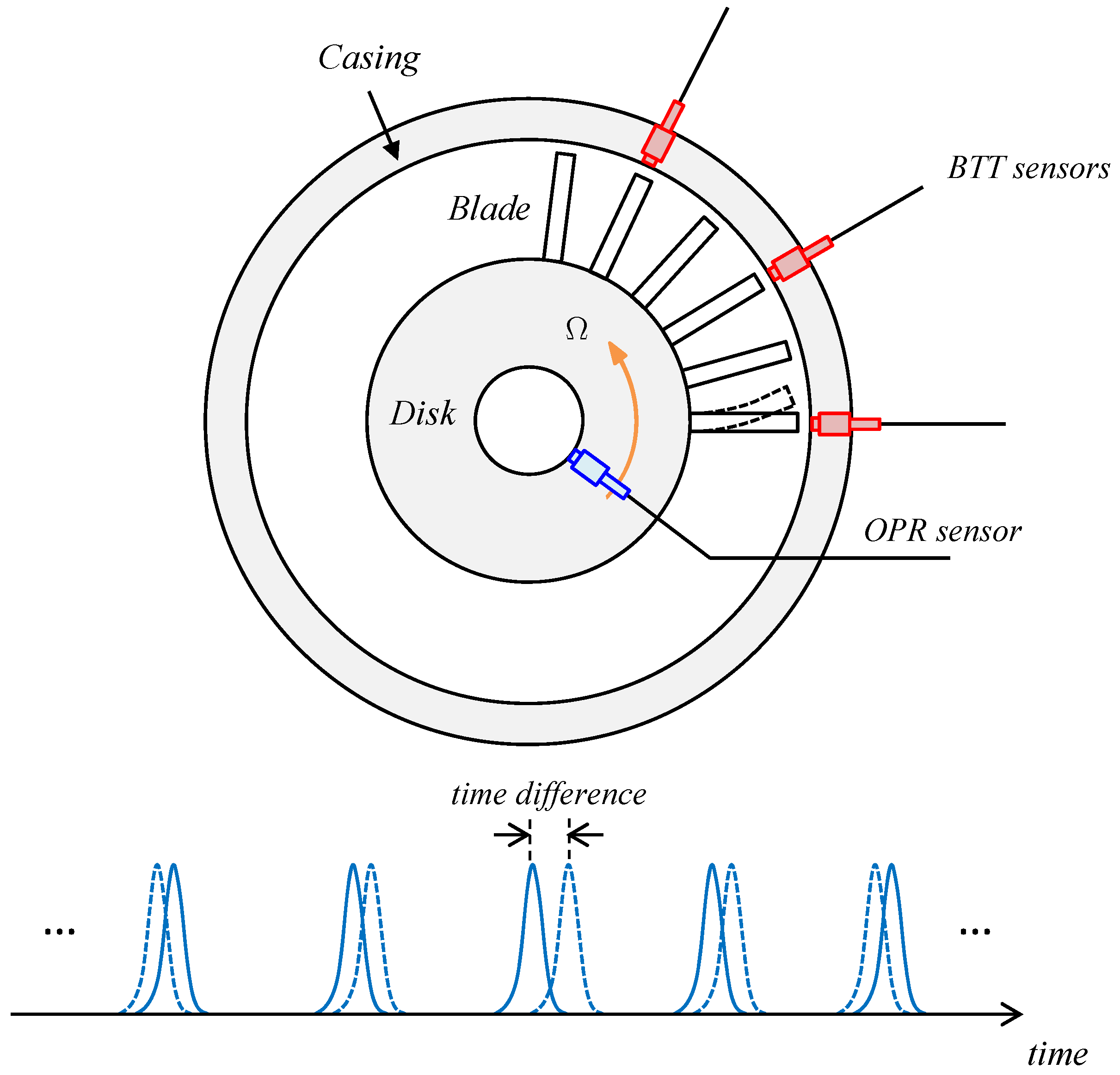
2.1. Tip Timing Basic Principles

BTT is a non-intrusive measurement technique, very promising for vibration monitoring of turbomachinery rotor blades. The method is based on the concept of the time of arrival of a vibrating blade. When the blades are vibrating, they pass in front of each sensor at a different time (time of arrival), compared to not vibrating blades. Actually, compared to a not vibrating blade, a vibrating blade will arrive at each sensor slightly earlier or later. By calculating the difference of time of arrival for vibrating and non-vibrating blades, the blade tip deflection can be evaluated. The blade deflection signal is the basis of the rest of the analysis. By post-processing this signal, the vibration properties can be determined.

A typical scheme of a BTT measurement system for blade vibration detection is depicted in Figure 1. As shown, BTT sensors are mounted on the stationary casing and arranged circumferentially around the rotor blades. The number of sensors and their arrangement are chosen based on the values of the natural frequencies, the number of modes and the EO of excitation.

2.2. Two Degrees of Freedom Fitting Method

One of the first methods proposed to fit tip-timing data is the single parameter method [9]. This method was developed based on the SDOF resonator model but it is only valid for a system with a single mode resonance. By fitting the SDOF model to the blade tip deflection at resonance, the vibration parameters can be determined. However, this method is not suitable in cases where two close resonance peaks are present. Two close peaks are quite common in the dynamic response of bladed disk. This happens when the frequency of one mode is split in two closely-spaced frequencies due to mistuning, or when two or more modes with close frequency are excited simultaneously by different EOs. In fact, in these conditions the blade response is dominated by only two modes’ contribution around the resonance region. Therefore, the vibration response of the blade near the resonance can be modeled by only considering these two modes. Thus, by using the modal analysis technique [22,23], the equations of motion of the blades can be represented by just two uncoupled equations in terms of generalized coordinates (modal coordinates). Each uncoupled equation in the modal coordinates is of the SDOF type. The solution in the original (physical) coordinate is obtained by the sum of the modal solutions of each SDOF system. Indeed, the concept is an extension of the SDOF method to 2DOF system. The procedure is explained in detail below.

Based on the modal analysis technique, the motion related to each mode ${\varphi }_i$ of a vibrating system can be represented by generalized coordinates, ${\eta }_i$. Accordingly, the equations of motion of the system for the forced response oscillation can be written as

$${\ddot{\eta }}_i+2{\zeta }_i{\omega }_{n_i}{\dot{\eta }}_i+{\omega }_{n_i}^2{\eta }_i=Q_i\left(t\right),i=1,2,\dots ,m$$

(1)

where ${\zeta }_i$, ${\omega }_{n_i}$ and $Q_i\left(t\right)$ respectively are the damping ratio, natural frequency and the generalized force (modal force) corresponding to the ith mode.

Equation (1) represents a set of m uncoupled equations and each equation can be treated as an SDOF system. The steady state response of an SDOF system under harmonic excitation $Q_i\left(t\right)={\overline{Q}}_{i}cos(\omega t+{\overline{\psi }}_i)$ is given by

$${\eta }_i\left(t\right)={\overline{\eta }}_{i}cos\left(\omega t+{\overline{\psi }}_i-{\phi }_i\right)$$

(2)

in which

$${\overline{\eta }}_i=\frac{{\delta }_i}{\sqrt{\left(1-r_i^2\right)+{\left(2{\zeta }_i{r}_i\right)}^2}};{\phi }_i=\frac{2{\zeta }_i{r}_i}{1-r_i^2};r_i=\frac{\omega }{{\omega }_{n_i}};{\delta }_i=\frac{{\overline{Q}}_i}{{\omega }_{n_i}^2}$$

(3)

$\omega$ is the excitation frequency and ${\overline{\psi }}_i$ is the initial phase angle in the forcing function.

Finally, the response of the system can be obtained by the linear combination of the normal modes of the system, ${\varphi }_i$. When the contribution of two modes is present which corresponds to the particular case of $m=2$, the response of the system in the physical coordinate, $y\left(t\right)$, at an arbitrary point can be expressed as

$$y\left(t\right)={\varphi }_1{\eta }_1\left(t\right)+{\varphi }_2{\eta }_2\left(t\right)$$

(4)

When the blade passes in front of a sensor located at an arbitrary angular position, $\theta$, the phase angle $\omega t$ at the kth rotation can be written as

$${\left(\omega t\right)}_k=EO\left(\epsilon +\theta +2\pi k\right)$$

(5)

where $\epsilon$ is the angular position of the blade at $t=0$.

By substituting Equation (5) into Equation (4), the blade tip response measured by the sensor is stated as

$$\begin{array}{c}{y}_k=\frac{{\overline{\delta }}_1}{\sqrt{\left(1-r_{1k}^2\right)+{\left(2{\zeta }_1{r}_{1k}\right)}^2}}cos\left(EO\theta +{\psi }_1-{\phi }_1\left(r_{1k}\right)\right)\hfill \\ +\frac{{\overline{\delta }}_2}{\sqrt{\left(1-r_{2k}^2\right)+{\left(2{\zeta }_2{r}_{2k}\right)}^2}}cos\left(EO\theta +{\psi }_2-{\phi }_2\left(r_{2k}\right)\right)\hfill \end{array}$$

(6)

in which ${\overline{\delta }}_1={\varphi }_1{\delta }_1$ and ${\overline{\delta }}_2={\varphi }_2{\delta }_2$. In addition, ${\psi }_1$ and ${\psi }_2$ incorporate the parameters $\epsilon$ and ${\overline{\psi }}_i$, given as

$${\psi }_i=\epsilon +{\overline{\psi }}_i,i=1,2$$

(7)

2.3. Fitting Procedure

The 2DOF model represented by Equation (6) can now be fitted into the BTT sensors data and the vibration parameters of the blades can be identified by this procedure. Figure 2 shows in gray a typical response of the blade in the case of one isolated resonance. The blue and red curves are the displacement curves detected by the two sensors. The data of the two sensors curves can be fitted with the Equation (6). Starting from an estimated value of EO, the unknown parameters are determined by fitting analysis. The fitting unknowns include the natural frequencies $({\omega }_{n_1},{\omega }_{n_2})$, the damping ratios $({\zeta }_1,{\zeta }_2)$, the phase shifts $({\psi }_1,{\psi }_2)$ and the two parameters $({\overline{\delta }}_1,{\overline{\delta }}_2)$. The fitting analysis is carried out based on the nonlinear least square curve fitting technique. The value of residual from the least squares method indicates the goodness of fitting. By sweeping EOs and repeating the fitting process, the best curve fit and parameter estimation can be achieved. Defining constraints for unknown parameters reduce the computational cost and results in a faster and more accurate estimation of the parameters.

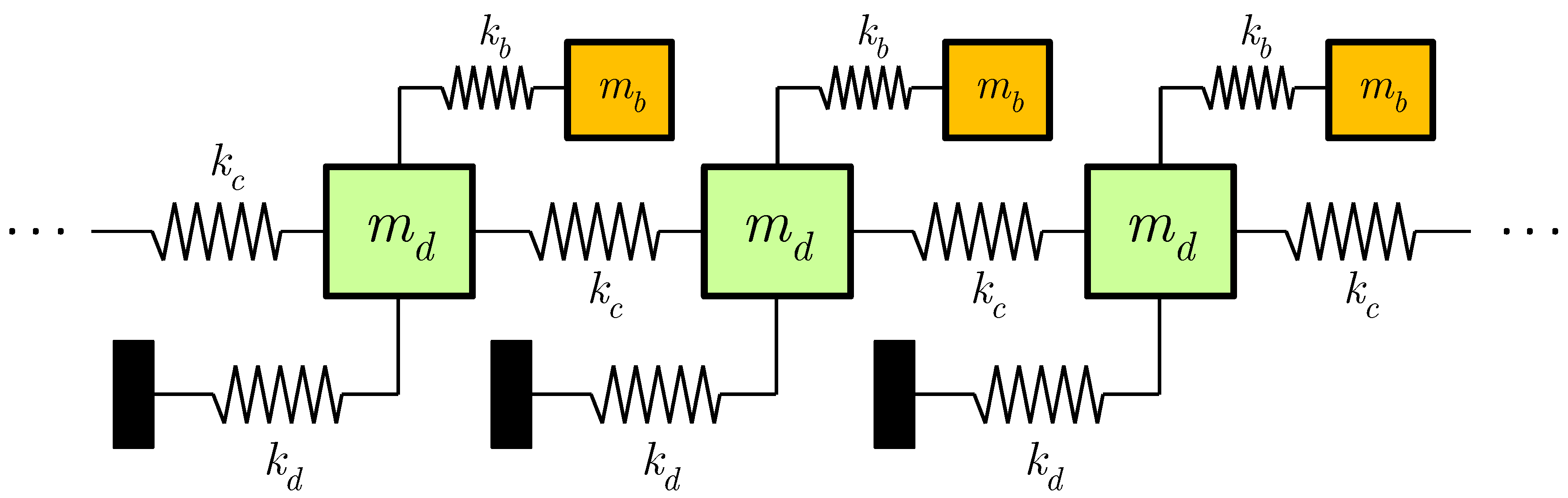
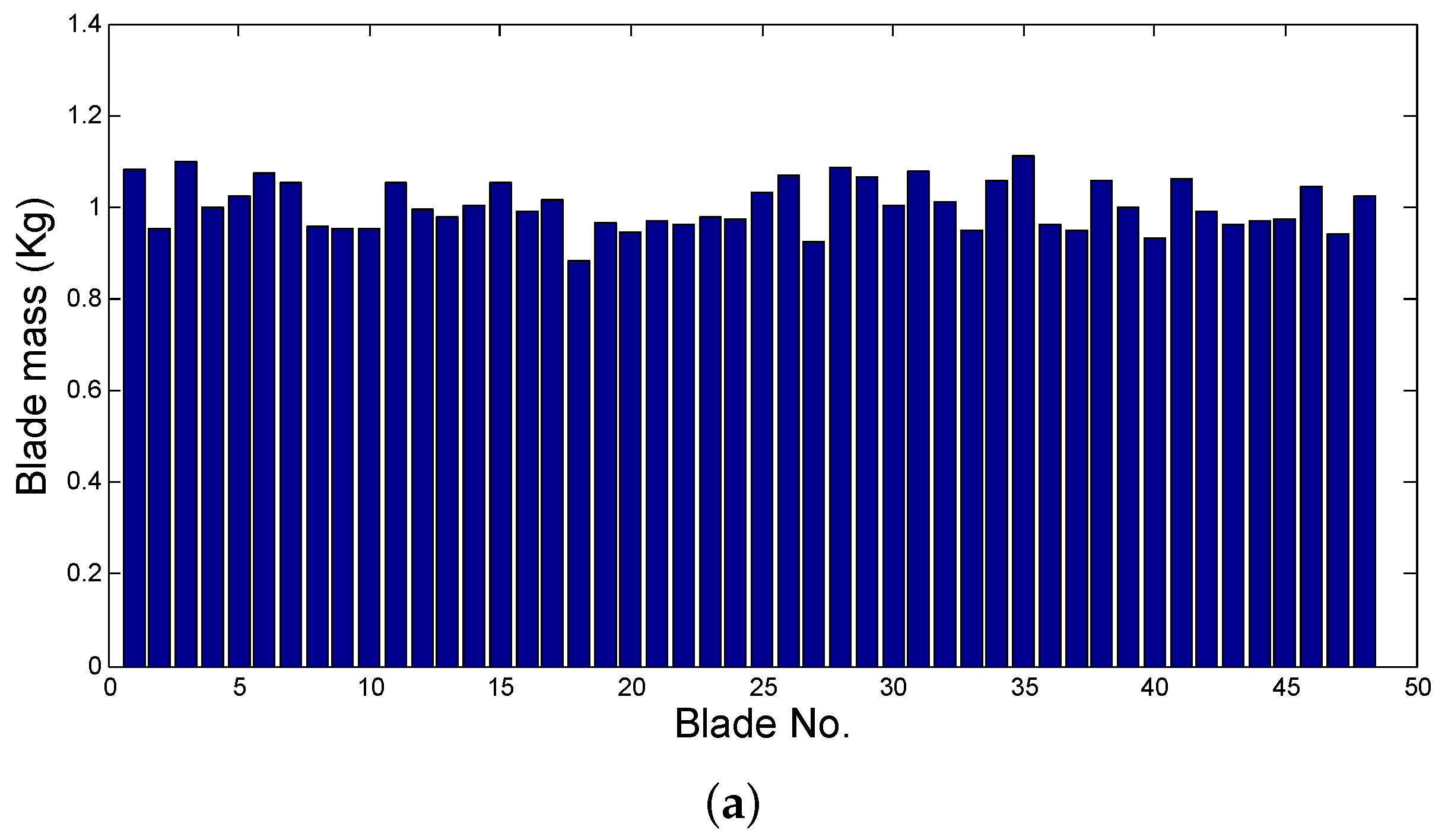
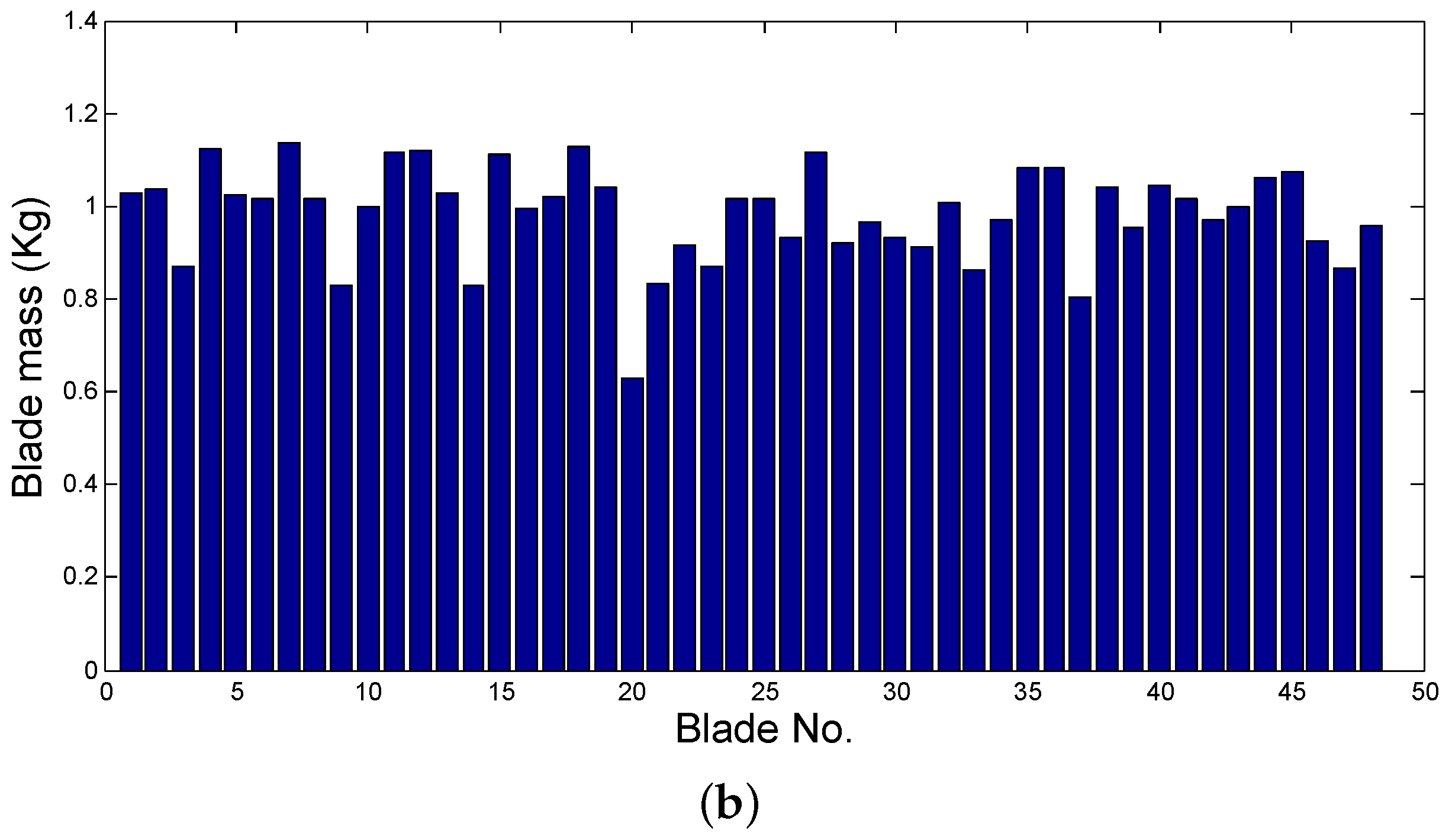
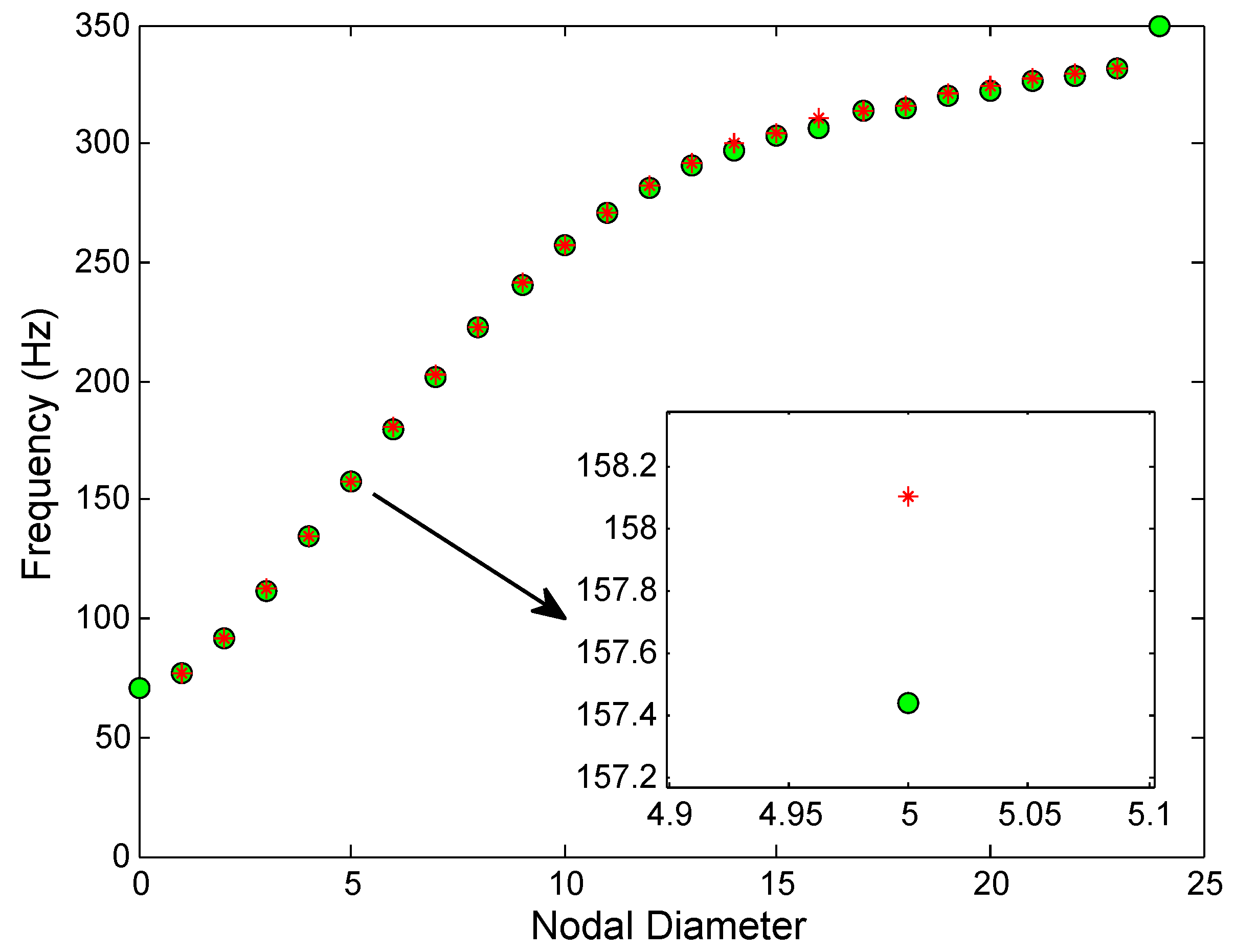
2.4. Reference Test Case

A lumped parameter model of a rotating bladed disk assembly is assumed as a test case for the verification of the method. This type of model was extensively used for investigating the effects of mistuning on the forced response of bladed disks [24,25,26,27]. Similar models [15,28] and models based on finite element method [10] were also employed by the researchers as numerical simulators for generating the tip timing data in order to test their analysis methods. Figure 3 shows a schematic representation of a lumped parameter model. In the model two degrees of freedom are considered for each bladed disk sector (one for the blade and one for the disk sector). Each sector is attached to its neighboring sectors by the coupling springs, $k_c$. To avoid rigid body motion, an extra spring, $k_d$, connects each sector to the ground. The masses of the blade and the disk in each sector are respectively denoted by $m_b$ and $m_d$, and $k_b$ represents the blade stiffness.

The equations of motion for the bladed disk system can be written as:

$$\mathbf{M}\ddot{\mathbf{q}}\left(t\right)+\mathbf{C}\ddot{\mathbf{q}}\left(t\right)+\mathbf{Kq}\left(t\right)=\mathbf{F}\left(t\right)$$

(8)

where $\mathbf{M}$, $\mathbf{C}$ and $\mathbf{K}$ represent the mass, damping and stiffness matrices, while $\mathbf{q}$ and $\mathbf{F}$ denote the displacement and external force vectors, respectively. Very similar models with the same matrices of Equation (8) can be found in [24,29]. Damping matrix is constructed according to the proportional damping model ($\mathbf{C}=\alpha \mathbf{M}+\beta \mathbf{K}$) in which $\alpha$ and $\beta$ are known constants.

The excitation force is assumed as a traveling wave excitation force acting on each blade. The force can be written as:

$$\begin{array}{c}{f}_i\left(t\right)=f_{0}cos\left(\omega t-\frac{2\pi EO}{N}\left(i-1\right)\right);i=1,2,3,\dots ,N\end{array}$$

(9)

where N is the total number of blades and $f_0$ is the amplitude of excitation. The excitation frequency is given by $\omega =EO.\mathsf{\Omega }$, where $\mathsf{\Omega }$ denotes the rotating speed.

A typical case of dual mode resonance, is the splitting frequency phenomenon [25,30] which takes place in a mistuned bladed disk assembly. Mistuning is caused by small unavoidable imperfections in manufacturing process or by deviation of the components from their ideal design shape due to machine operation which eventually breaks the cyclic symmetric features of the system. One major consequence of the mistuning is the splitting of the frequencies of two orthogonal modes. In the tuned system the two orthogonal modes have the same natural frequency. When the symmetry of the system is lost due to mistuning, two frequencies are separated from each other and the corresponding modes appear as two distinct modes with the same nodal diameter. In Figure 4, it is displayed how this phenomenon appears in a Campbell diagram where there are two close lines instead of one for a given mode shape (same nodal diameter). This will cause the excitation of two close resonances by the same EO at two different rotational speeds.

Here a bladed disk assembly is assumed as a test case consisting of 48 blades equally spaced around the disk. The parameters for the bladed disk model are given in

Table 1. Parameters of the bladed disk model.

Parameter	Symbol	Value	Unit
Single blade mass	$m_b$	1	kg
Disk sector mass	$m_d$	4	kg
Blade stiffness	$k_b$	5 × 10${}^6$	N/m
Disk stiffness	$k_d$	1 × 10${}^6$	N/m
Coupling stiffness	$k_c$	1 × 10${}^7$	N/m

. The BTT sample signals are acquired by two virtual sensors located at the angles of 0 and $\pi /4$. A pattern of imperfections with respect to the tuned system is applied in order to induce the mistuning. Indeed, the mistuning is applied to the assembly based on a random distribution of the blade mass with the standard deviation (SD) of $0.05$ in one case and $0.10$ in the other case. The mistuning patterns for the two cases are shown in Figure 5. The natural frequencies of the bladed disk for the mistuned configuration with $SD=0.10$ is plotted in the diagram frequency vs. nodal diameters in Figure 6. The effect of mistuning can be observed here as a frequency splitting of a few tenths of Hertz in the frequency for all the nodal diameters, except 0 and 24. The close up in Figure 6 shows the frequency splitting for nodal diameter 5.

2.5. Generation of Sampled Data

Now, by considering the traveling wave excitation of Equation (9), the steady state response of the bladed disk system can be obtained by Equation (8). The gray curve in Figure 2 typically shows such steady state response. From the point of view of the sensors, in the stationary frame, the BTT samples are acquired once per revolution. The time of arrivals for each sensor in each revolution can be calculated by Equation (5). Then, the response of the system corresponding to the calculated time of arrivals is simply selected from the blade response reflected in the gray curve. In this way, the signals detected by the sensors can be simulated, in Figure 2 the blue and red curves represents such sensors simulated data.

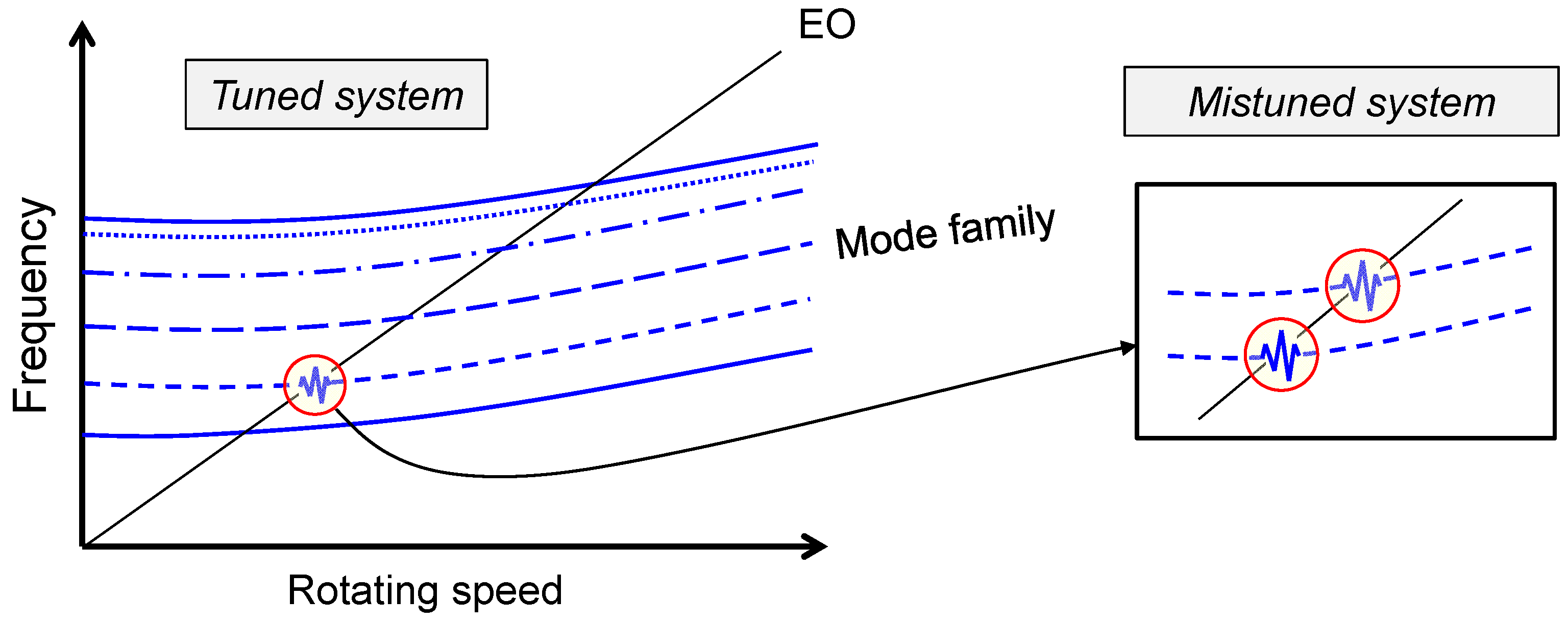
3. Discussion of Results

In order to validate the curve fitting algorithm based on the 2DOF model, BTT sampled data in different resonance conditions are generated by the numerical simulator introduced in the previous section. For all the test cases investigated hereafter, the proportional damping constant $\alpha$ is always set to zero, while only the parameter $\beta$ is changed. For providing a better understanding, the corresponding damping ratios $\zeta$ have been reported instead of $\beta$ [31].

The results obtained with the proposed 2DOF algorithm are here compared with those obtained by the classical “Sine fitting method” used in many commercial softwares. The two methods are here used to reconstruct the frequency response for a certain mode starting from the sensors data. The reconstructed response will then be compared with the response curve obtained by the mathematical model.

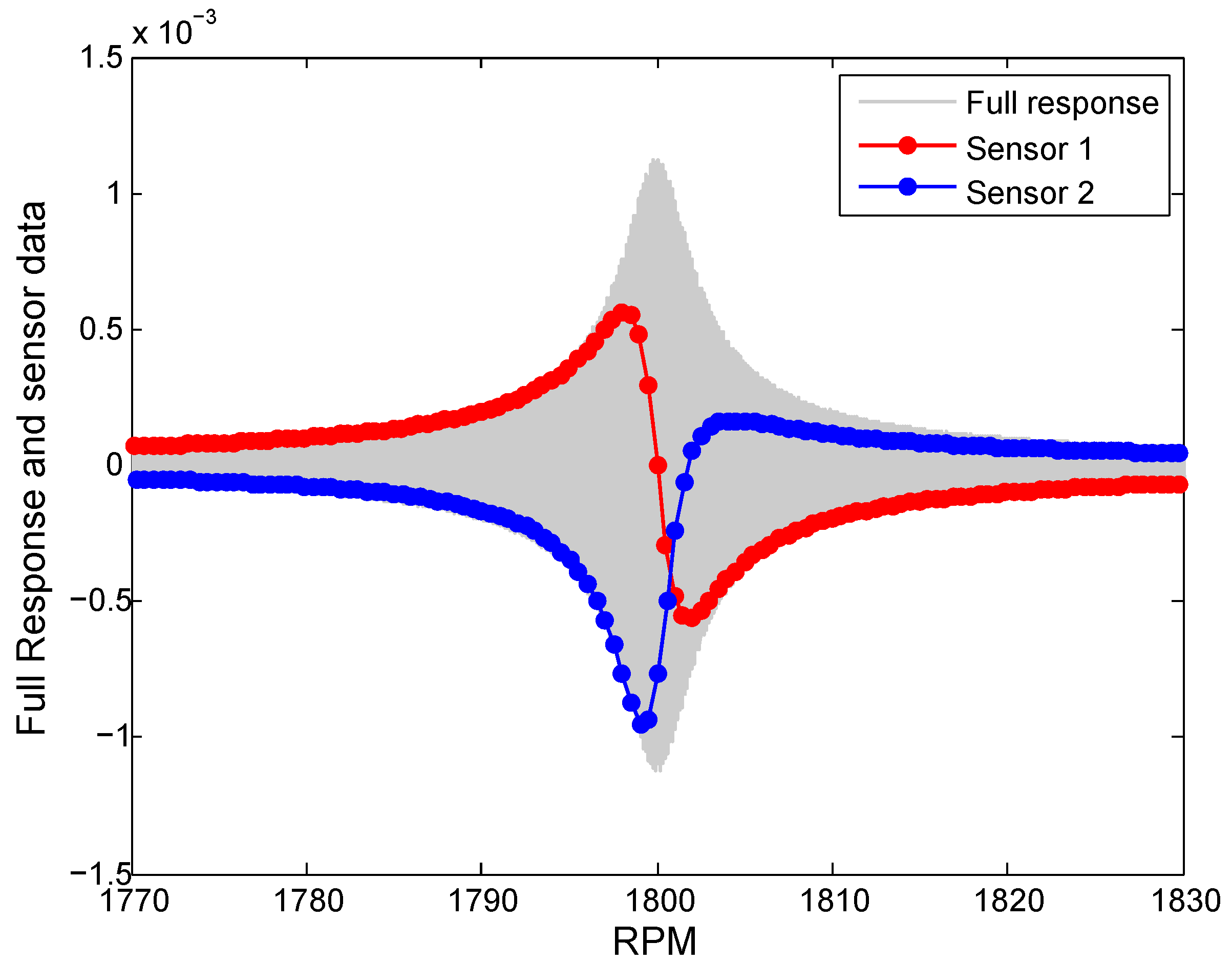
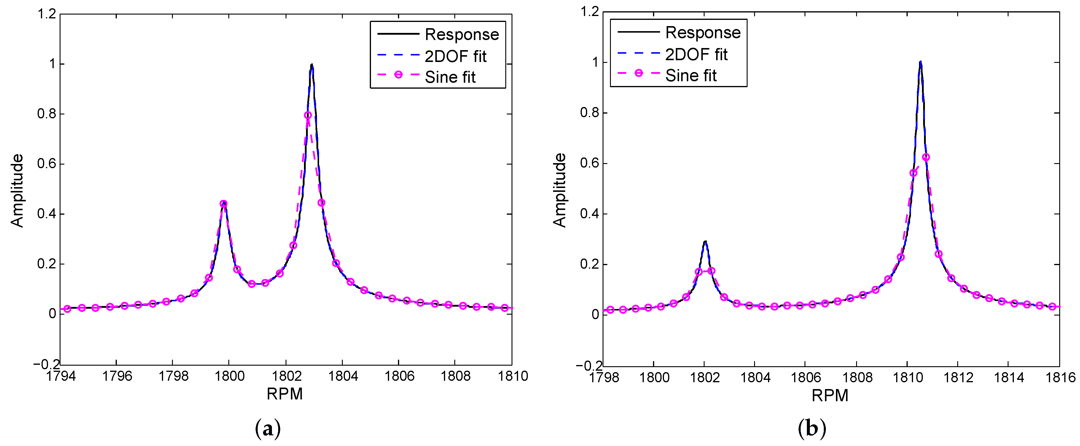
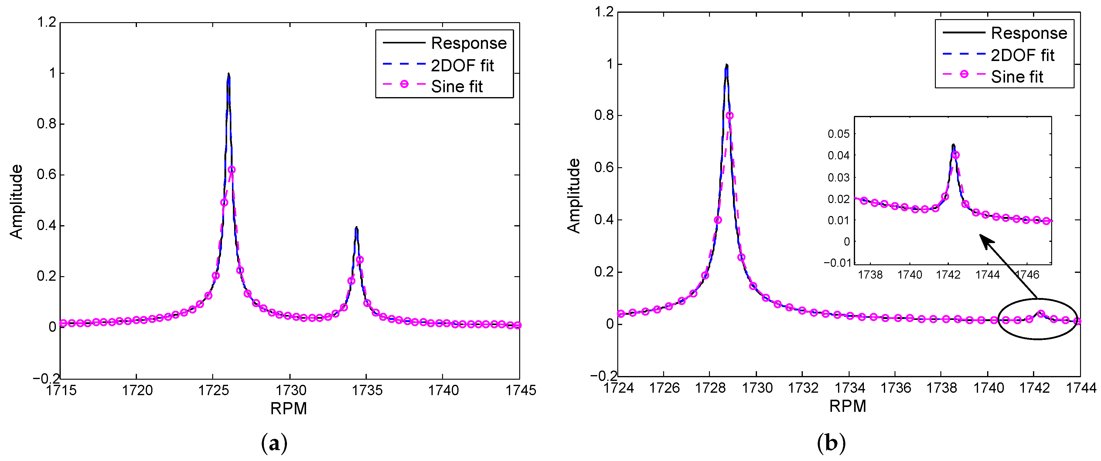
3.1. Low Damping Case

The first case considered is that with low damping (${\zeta }_{1,2}=0.0001$) and well-separated modes. The vibrating mode is the one corresponding to the first family at ND = 5. Due to mistuning the EO = 5 excitation produces two frequency response peaks at two different rotational speeds. Figure 7 shows the response computed mathematically (continuous line) overlapped on the reconstructed response curves (dotted lines) using both fitting methods (2DOF fit and Sine fitting). The two figures correspond to the two different random mass distribution patterns. It can be seen that there is an excellent match between the curve obtained by the 2DOF fitting and the original response. In comparison to the Sine fit method, the 2DOF method better capture the amplitude of the two resonance peaks. The parameters directly obtained by the fitting procedure with the 2DOF model are the resonance frequencies and the damping ratios. The obtained values can be compared to the real ones set in the mathematical model. The frequency and damping values identified by the 2DOF fitting method are listed in

Table 2. Comparison of vibration parameters identified by the 2 degrees of freedom (2DOF) fit model with the exact values for Engine Order (EO) = 5.

Parameters	SD = 0.05			SD = 0.10
	Exact Value	Calculated	Difference (%)	Exact Value	Calculated	Difference (%)
Frequency 1	157.1322	157.1322	0.00	157.4456	157.4456	0.00
Frequency 2	157.6046	157.6046	0.00	158.1039	158.1039	0.00
Damping 1	0.00009985	0.00009987	0.02	0.00009979	0.00009981	0.02
Damping 2	0.00010015	0.00010000	0.15	0.00010021	0.00010017	0.04
Residual	5.3537 × 10${}^{-6}$			1.6128 × 10${}^{-6}$

and compared to the exact values of the mathematical model. The comparison of the values confirms the good estimation obtained by the 2DOF model, the value of residual close to zero confirms the good quality of fitting.

In a second step of computation, modes corresponding to higher nodal diameters are considered in particular modes corresponding to ND = 6, 7, 10 excited by the corresponding EO. As in the previous case, for each nodal diameter there is a splitting of the two resonance frequencies excited at two different rotational speeds. The response curves (the mathematical one and the two curves obtained by fitting) are shown in Figure 8, Figure 9 and Figure 10. For all the cases it is confirmed that the 2DOF method predicts the amplitude of the response at resonance better than the Sine fitting method. This difference can be attributed to the fact that the Sine fitting method is influenced by the sampling frequency of the signal. Since the BTT signals are sampled once per revolution, for the Sine fit method more samples are needed to successfully cover the whole range of the resonance. Particularly for sharp peaks (small damping) close to the resonance a higher sampling rate would be required. This can be achieved by reducing the acceleration/deceleration rate which is considered here with a realistic value of 0.25 Hz/s. On the contrary the 2DOF method is not so sensitive to the BTT sampling frequency since it uses the data of the entire resonance region to be fitted by using the mathematical formula of Equation (6). In the particular cases, as the proposed examples, of sharp amplitude peaks with low damping values, applying only the Sine fitting method might be inadequate with the risk of underestimating the amplitude of the peaks. In these cases the 2DOF method proved to be a good numerical tool to verify and to correct the results of the Sine fitting method.

For evaluating in more detail the performance of the 2DOF fitting model, further cases have been investigated with different damping properties. Increasing damping reduces the vibration amplitudes and, as a consequence, one large peak could be present instead of two peaks, even if for a single mode the peaks should be split due to mistuning. In this condition, the curve fitting and the parameters identification become complicated. Figure 11 shows the fitted curves for damping ratios of $0.002$ and $0.003$ for two different EOs. Since in this case only one peak seems to be present, the fitting was also done with the SDOF method. It can be observed that both 2DOF and Sine fit models exhibit perfect approximations. On the contrary, the 1DOF model is not able to completely capture the response since the model 1DOF is not correct, being here two peaks partially overlapped. The values of the identified parameters (resonance frequency and damping) using both 2DOF and 1DOF model are also listed in

Table 3. Comparison of vibration parameters identified by 2DOF and 1DOF models with the exact values for EO = 5, 8 and SD = 0.10.

		2DOF		1DOF
		EO = 5
Parameters	Exact Value	Calculated	Difference (%)	Calculated	Difference (%)
Frequency 1	157.4456	157.4470	0.00	157.6627	0.14
Frequency 2	158.1039	158.1063	0.00	—	—
Damping 1	0.001995	0.001987	0.40	0.002243	12.39
Damping 2	0.002004	0.002006	0.13	—	—
		EO = 8
Frequency 1	222.3561	222.3663	0.00	222.2287	0.35
Frequency 2	223.0106	222.9823	0.01	—	—
Damping 1	0.002995	0.002988	0.24	0.004071	35.91
Damping 2	0.003004	0.003018	0.46	—	—

. It can be observed that the 2DOF evaluation method is able to accurately identify the vibration parameters for each mode, whereas the 1DOF model provides a good prediction for frequency but overestimate damping. It should be noticed that in the case of the Sine fitting method the same parameters are not obtained directly by the fitting procedure, in fact in this case the resonance frequency and the associated damping are estimated not during the fitting but after, by post processing the obtained reconstructed response curve. The damping can be obtained by means of techniques like half-power method, but in a case like this, where two close peaks are partially overlapped, using half-power method can lead to not accurate results. More accurate results can be reached by doing a further FRF curve fit analysis [32,33,34] which takes extra effort. However, in particular for the identification of the damping value associated to a certain resonance, the 2DOF method gives more accurate results than Sine fitting (based on half-power method), because the damping parameters are variables of the model obtained directly by the fitting procedure. This holds if the experimenter uses the appropriate model, that is 2DOF instead of 1DOF model when the shape of the peak suggests that there might be two partially overlapping peaks due to the presence of mistuning.

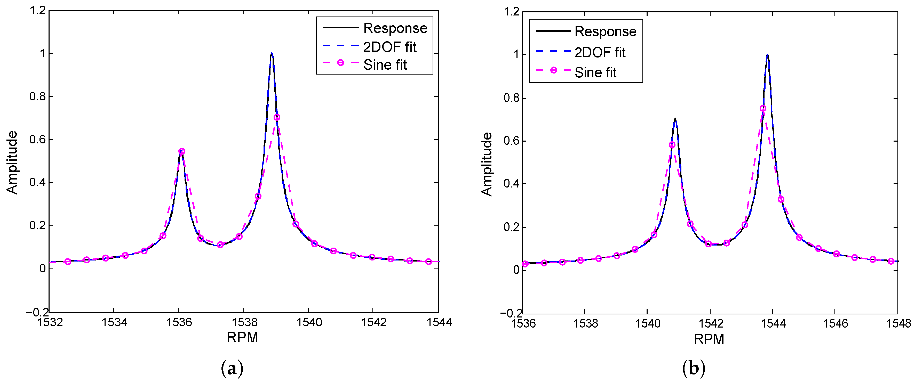
3.2. High Damping Case

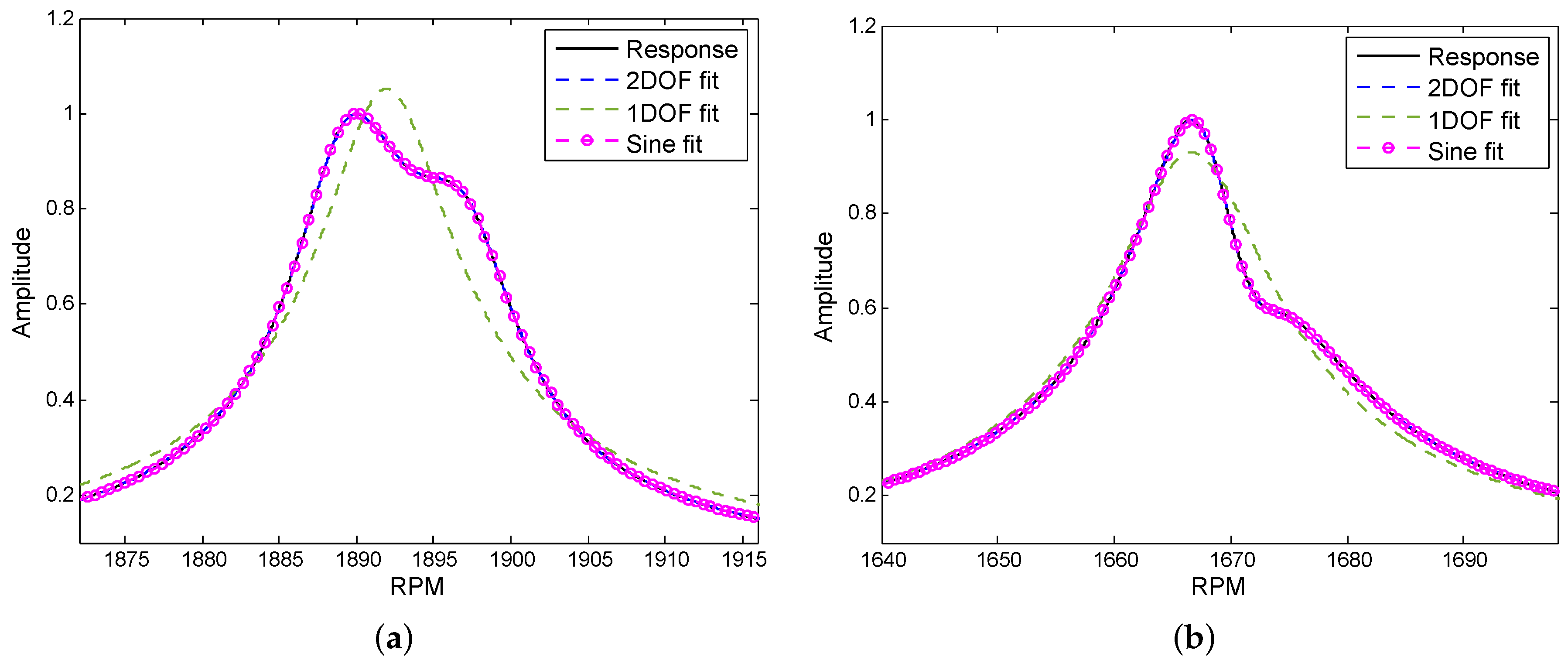
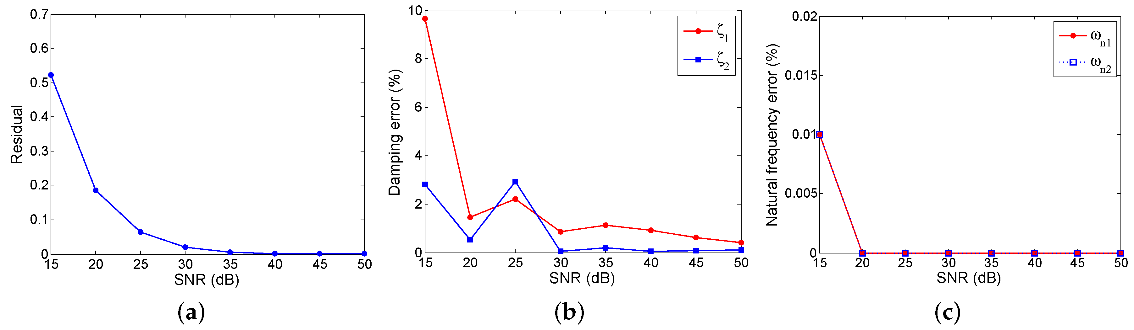
In real operating conditions it could happen that the damping is even higher than the previous cases. In this condition the two close peaks due to mistuning appear as completely merged in one single peak. Figure 12 shows the results of the fitting process for such condition. It can be seen that the original response is successfully reconstructed both by the 2DOF and by the Sine fit method. However, it should be highlighted that in a case like this where the two peaks are completely merged together, the 2DOF method is comparable to the Sine fitting for the estimation of the response curve but it is not better in the estimation of the vibration parameters, in particular the damping. In this case in fact, the 2DOF least square curve fitting optimizer might not always return the vibrations parameters with the high accuracy as in Table 3.

3.3. Noisy Signals

As a last step, noise was added to the simulated sensors data in order to evaluate the noise effects on the fitting accuracy of the 2DOF method. Figure 13 shows the sensors data contaminated by noise. This noise was assumed as an additive white Gaussian noise from the analysis of the typical noise patterns of the BTT sensors signals in literature [16,35,36,37]. The typical noise pattern adds dynamic disturbances to the signal, without changing the overall behavior of the signal. The influence of noise on the residual is plotted in Figure 14a. As expected, by increasing the noise level, that is by decreasing the Signal-to-Noise Ratio (SNR), the residual from the curve fitting increases, that is the quality of fitting becomes worst. The errors in the estimated damping values are depicted versus the SNR in Figure 14b. It can be seen that beyond an SNR level of 20 dB (see Figure 13a), the error on the damping value estimation is below 5%, which is an acceptable value from an engineering point of view. The errors in the estimated natural frequencies are depicted in Figure 14c against the SNR. In this case the error is always much lower than 1% which is almost negligible.

4. Conclusions

The paper is focused on the post processing procedure of the BTT sensors data in the case where two very close resonance frequencies are present in the dynamic response of the rotating system. Having two close resonance peaks is the typical case of the dynamic response of a bladed disk in presence of mistuning, due for example to an asymmetry of the distribution of the mass in the disk. In this case, having an instrument that can fit the experimental data to obtain the main vibration parameters (resonance frequencies and damping) for both the modes associated to the close resonances is very useful to the experimenter or to the designer. A method based on the nonlinear least square fitting of the sensors data by a 2DOF dynamic model was here presented. A lumped parameter model representing a rotating mistuned bladed disk assembly was used as a test case. The sensors measurement data were simulated numerically. The results obtained by the 2DOF fitting method are compared with those obtained by the most classical Sine fitting method employed in the majority of the BTT commercial systems. The following main conclusions can be drawn.

-

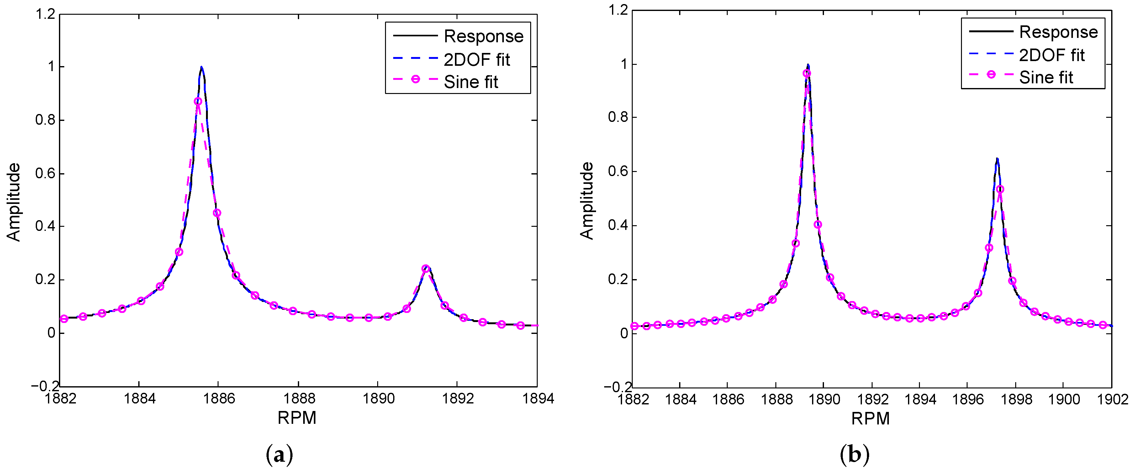
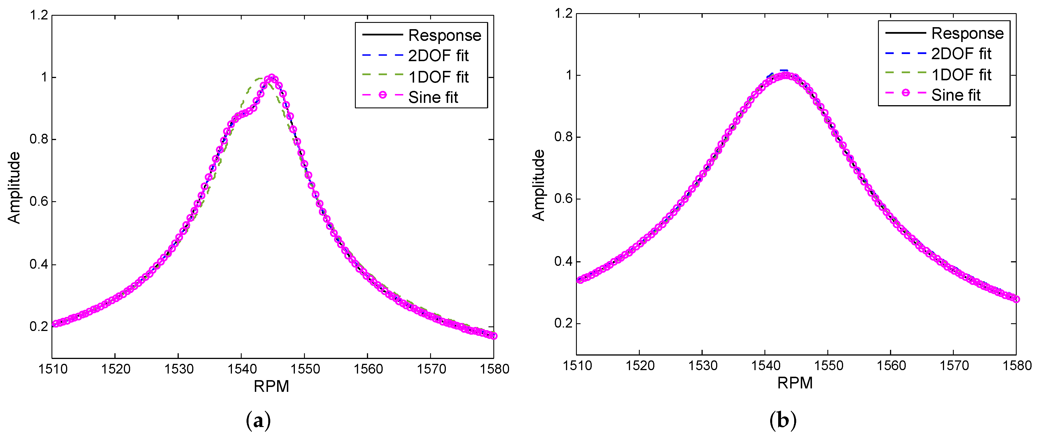
The 2DOF fitting method is more accurate than the Sine fit method in the determination of the maximum response amplitude when the two peaks are very sharp and well separated since the damping is very low ($\zeta =0.0001$). In this case, the 2DOF model can directly estimate the fitting parameters, damping value and resonance frequency, associated to each peak with an accuracy lower than 1%. The Sine fit method is less accurate since it is sensitive to the number of samples of the BTT data which is considerably affected by the rate of acceleration or deceleration, while the 2DOF method is not so sensitive to the sampling rate since it is based on a mathematical model of the response curve.

-

As the damping increases ($\zeta$ = 0.002–0.003), the two peaks have more overlap and appear as a wider peak. In this case the 2DOF method has the same accuracy as the Sine fitting method in estimating the amplitude of the response. In addition, the 2DOF method is able to estimate the damping value directly from the fitting with errors still less than 1%. In the presence of noise (with SNR higher than 20 dB) the error remains below 5%. On the contrary the Sine fit method does not get the damping value directly from the fitting but requires to estimate the damping from the width of the peak itself and this estimate can be altered by the fact that there are two overlapped peaks.

-

For even higher damping values ($\zeta =0.006$) when only one single peak is visible because the two peaks are merged, the two methods (2DOF and Sine fit) are equivalent. The 2DOF method can no longer obtain the damping values associated with the two modes with the same accuracy as in the previous cases.

The 2DOF method therefore seems to be a valid method to be used in the case of close resonance peaks if the experimenter wants to determine not only the shape and the amplitude of the response peak but also the system parameters (resonance frequencies and damping). Employing this method as a separate module or as a complementary plugin along with the traditional BTT methods such as Sine fit method can be an added value to the measurement system.

References

1. Gonzalez-Barrio, H.; Calleja-Ochoa, A.; Lamikiz, A.; Lopez de Lacalle, L. Manufacturing Processes of Integral Blade Rotors for Turbomachinery, Processes and New Approaches. Appl. Sci. 2020, 10, 3063. [Google Scholar] [CrossRef]
2. Russhard, P. The rise and fall of the rotor blade strain gauge. In Vibration Engineering and Technology of Machinery; Springer: Berlin/Heidelberg, Germany, 2015; pp. 27–37. [Google Scholar]
3. Knappett, D.; Garcia, J. Blade tip timing and strain gauge correlation on compressor blades. Proc. Inst. Mech. Eng. Part G J. Aerosp. Eng. 2008, 222, 497–506. [Google Scholar] [CrossRef]
4. Tomassini, R.; Rossi, G.; Brouckaert, J.F. On the development of a magnetoresistive sensor for blade tip timing and blade tip clearance measurement systems. Rev. Sci. Instrum. 2016, 87, 102505. [Google Scholar] [CrossRef] [PubMed]
5. Jamia, N.; Friswell, M.I.; El-Borgi, S.; Rajendran, P. Modelling and experimental validation of active and passive eddy current sensors for blade tip timing. Sens. Actuators A Phys. 2019, 285, 98–110. [Google Scholar] [CrossRef] [Green Version]
6. Chen, Z.; Yang, Y.; Xie, Y.; Guo, B.; Hu, Z. Non-contact crack detection of high-speed blades based on principal component analysis and Euclidian angles using optical-fiber sensors. Sens. Actuators A Phys. 2013, 201, 66–72. [Google Scholar] [CrossRef]
7. Abdul-Aziz, A.; Woike, M.R.; Clem, M.; Baaklini, G. Engine rotor health monitoring: An experimental approach to fault detection and durability assessment. In Proceedings of the Smart Sensor Phenomena, Technology, Networks, and Systems Integration 2015, San Diego, CA, USA, 8–12 March 2015; Volume 9436, p. 94360A. [Google Scholar]
8. Rzadkowski, R.; Rokicki, E.; Piechowski, L.; Szczepanik, R. Analysis of middle bearing failure in rotor jet engine using tip-timing and tip-clearance techniques. Mech. Syst. Signal Process. 2016, 76, 213–227. [Google Scholar] [CrossRef]
9. Zablotskiy, I.Y.; Korostelev, Y.A. Measurement of Resonance Vibrations of Turbine Blades with the ELURA Device; Technical Report; Foreign Technology Div Wright-Patterson AFB: Dayton, OH, USA, 1978. [Google Scholar]
10. Heath, S.; Imregun, M. An improved single-parameter tip-timing method for turbomachinery blade vibration measurements using optical laser probes. Int. J. Mech. Sci. 1996, 38, 1047–1058. [Google Scholar] [CrossRef]
11. Heath, S. A new technique for identifying synchronous resonances using tip-timing. J. Eng. Gas Turbines Power 2000, 122, 219–225. [Google Scholar] [CrossRef]
12. Schlagwein, G.; Schaber, U. Non-contact blade vibration measurement analysis using a multi-degree-of-freedom model. Proc. Inst. Mech. Eng. Part A J. Power Energy 2006, 220, 611–618. [Google Scholar] [CrossRef]
13. Rigosi, G.; Battiato, G.; Berruti, T.M. Synchronous vibration parameters identification by tip timing measurements. Mech. Res. Commun. 2017, 79, 7–14. [Google Scholar] [CrossRef] [Green Version]
14. Heath, S. A Study of Tip-Timing Measurement Techniques for the Determination of Bladed-Disk Vibration Characteristics. Ph.D. Thesis, University of London, London, UK, 1997. [Google Scholar]
15. Carrington, I.B.; Wright, J.R.; Cooper, J.; Dimitriadis, G. A comparison of blade tip timing data analysis methods. Proc. Inst. Mech. Eng. Part G J. Aerosp. Eng. 2001, 215, 301–312. [Google Scholar] [CrossRef]
16. Russhard, P. Development of a Blade Tip Timing Based Engine Health Monitoring System; The University of Manchester: Manchester, UK, 2010. [Google Scholar]
17. Guo, H.; Duan, F.; Zhang, J. Blade resonance parameter identification based on tip-timing method without the once-per revolution sensor. Mech. Syst. Signal Process. 2016, 66–67, 625–639. [Google Scholar] [CrossRef]
18. Heller, D.; Sever, I.; Schwingshackl, C. A method for multi-harmonic vibration analysis of turbomachinery blades using Blade Tip-Timing and clearance sensor waveforms and optimization techniques. Mech. Syst. Signal Process. 2020, 142, 106741. [Google Scholar] [CrossRef]
19. Mohamed, M.; Bonello, P.; Russhard, P. A novel method for the determination of the change in blade tip timing probe sensing position due to steady movements. Mech. Syst. Signal Process. 2019, 126, 686–710. [Google Scholar] [CrossRef] [Green Version]
20. Battiato, G.; Firrone, C.; Berruti, T. Forced response of rotating bladed disks: Blade Tip-Timing measurements. Mech. Syst. Signal Process. 2017, 85, 912–926. [Google Scholar] [CrossRef]
21. Bornassi, S.; Ghalandari, M.; Maghrebi, S.F. Blade synchronous vibration measurements of a new upgraded heavy duty gas turbine MGT-70 (3) by using tip-timing method. Mech. Res. Commun. 2020, 104, 103484. [Google Scholar] [CrossRef]
22. Rao, S.S. Vibration of Continuous Systems; Wiley Online Library: Hoboken, NJ, USA, 2007; Volume 464. [Google Scholar]
23. Urbikain, G.; Campa, F.J.; Zulaika, J.J.; De Lacalle, L.N.L.; Alonso, M.A.; Collado, V. Preventing chatter vibrations in heavy-duty turning operations in large horizontal lathes. J. Sound Vib. 2015, 340, 317–330. [Google Scholar] [CrossRef]
24. Lee, S.Y.; Castanier, M.; Pierre, C. Assessment of probabilistic methods for mistuned bladed disk vibration. In Proceedings of the 46th AIAA/ASME/ASCE/AHS/ASC Structures, Structural Dynamics and Materials Conference, Austin, TX, USA, 18–21 April 2005; p. 1990. [Google Scholar]
25. Martel, C.; Corral, R. Asymptotic description of maximum mistuning amplification of bladed disk forced response. J. Eng. Gas Turbines Power 2009, 131, 022506. [Google Scholar] [CrossRef]
26. Kenyon, J.A.; Griffin, J. Experimental demonstration of maximum mistuned bladed disk forced response. In Proceedings of the Turbo Expo: Power for Land, Sea, and Air, Atlanta, GA, USA, 16–19 June 2003; Volume 36878, pp. 195–205. [Google Scholar]
27. Rivas-Guerra, A.J.; Mignolet, M. Local/global effects of mistuning on the forced response of bladed disks. J. Eng. Gas Turbines Power 2004, 126, 131–141. [Google Scholar] [CrossRef]
28. Dimitriadis, G.; Carrington, I.B.; Wright, J.R.; Cooper, J.E. Blade-tip timing measurement of synchronous vibrations of rotating bladed assemblies. Mech. Syst. Signal Process. 2002, 16, 599–622. [Google Scholar] [CrossRef]
29. Zhao, T.; Yuan, H.; Yang, W.; Sun, H. Genetic particle swarm parallel algorithm analysis of optimization arrangement on mistuned blades. Eng. Optim. 2017, 49, 2095–2116. [Google Scholar] [CrossRef]
30. Ewins, D.J. The effects of detuning upon the forced vibrations of bladed disks. J. Sound Vib. 1969, 9, 65–79. [Google Scholar] [CrossRef]
31. Fu, Z.F.; He, J. Modal Analysis; Elsevier: Amsterdam, The Netherlands, 2001. [Google Scholar]
32. Jeffers, T.; Kielb, J.; Abhari, R. A novel technique for the measurement of blade damping using piezoelectric actuators. In Turbo Expo 2000: Power for Land, Sea, and Air; American Society of Mechanical Engineers: New York, NY, USA, 2000. [Google Scholar]
33. Kielb, J.; Abhari, R.S. Experimental study of aerodynamic and structural damping in a full-scale rotating turbine. J. Eng. Gas Turbines Power 2003, 125, 102–112. [Google Scholar] [CrossRef]
34. Kammerer, A.; Abhari, R.S. Experimental study on impeller blade vibration during resonance—Part II: Blade damping. J. Eng. Gas Turbines Power 2009, 131, 022509. [Google Scholar] [CrossRef]
35. Wu, S.; Chen, X.; Russhard, P.; Yan, R.; Tian, S.; Wang, S.; Zhao, Z. Blade tip timing: From raw data to parameters identification. In Proceedings of the 2019 IEEE International Instrumentation and Measurement Technology Conference (I2MTC), Auckland, New Zealand, 20–23 May 2019; pp. 1–5. [Google Scholar]
36. Russhard, P. Blade tip timing (BTT) uncertainties. AIP Conf. Proc. 2016, 1740, 020003. [Google Scholar]
37. Jousselin, O. Development of Blade Tip Timing Techniques in Turbo Machinery; The University of Manchester: Manchester, UK, 2013. [Google Scholar]
Figure 1. Principle of the Blade Tip-Timing (BTT) method (solid line: non-vibrating blade, dashed line: vibrating blade).
Applsci 10 05930 g001
Figure 2. A typical blade response and BTT data during a resonance passage.
Applsci 10 05930 g002
Figure 3. Lumped parameter model of a bladed disk assembly used for simulation.
Applsci 10 05930 g003
Figure 4. Splitting frequency in a mistuned system.
Applsci 10 05930 g004
Figure 5. Mistuned distributions of the blade mass, (a) SD = 0.05, (b) SD = 0.10.
Applsci 10 05930 g005aApplsci 10 05930 g005b
Figure 6. Natural frequencies vs. nodal diameters for the simulated mistuned bladed disk (SD = 0.10).
Applsci 10 05930 g006
Figure 7. Comparison of non-dimensional amplitudes obtained by different fitting methods for EO = 5 and ζ 1 , 2 = 0.0001 , (a) SD = 0.05, (b) SD = 0.10.
Applsci 10 05930 g007
Figure 8. Comparison of non-dimensional amplitudes obtained by different fitting methods for EO = 6 and ζ 1 , 2 = 0.0001 , (a) SD = 0.05, (b) SD = 0.10.
Applsci 10 05930 g008
Figure 9. Comparison of non-dimensional amplitudes obtained by different fitting methods for EO = 7 and ζ 1 , 2 = 0.0001 , (a) SD = 0.05, (b) SD = 0.10.
Applsci 10 05930 g009
Figure 10. Comparison of non-dimensional amplitudes obtained by different fitting methods for EO = 10 and ζ 1 , 2 = 0.0001 , (a) SD = 0.05, (b) SD = 0.10.
Applsci 10 05930 g010
Figure 11. Comparison of non-dimensional amplitudes obtained by different fitting methods for SD = 0.10, (a) EO = 5, ζ 1 , 2 = 0.002 , (b) EO = 8, ζ 1 , 2 = 0.003 .
Applsci 10 05930 g011
Figure 12. Comparison of non-dimensional amplitudes obtained by different fitting methods for SD = 0.10, (a) EO = 10, ζ 1 , 2 = 0.003 , (b) EO = 10, ζ 1 , 2 = 0.006 .
Applsci 10 05930 g012
Figure 13. Typical sensor data contaminated by noise for EO = 5 and SD = 0.10, (a) Signal-to-Noise Ratio (SNR) = 20 dB, (b) SNR = 25 dB.
Applsci 10 05930 g013
Figure 14. Effect of noise on the fitting residual, damping ratio and natural frequency for EO = 5, ζ 1 , 2 = 0.002 and SD = 0.10, (a) fitting residual, (b) error in damping ratio, (c) error in natural frequency.
Applsci 10 05930 g014