Solving Partial Differential Equations Using Deep Learning and Physical Constraints

Abstract

The various studies of partial differential equations (PDEs) are hot topics of mathematical research. Among them, solving PDEs is a very important and difficult task. Since many partial differential equations do not have analytical solutions, numerical methods are widely used to solve PDEs. Although numerical methods have been widely used with good performance, researchers are still searching for new methods for solving partial differential equations. In recent years, deep learning has achieved great success in many fields, such as image classification and natural language processing. Studies have shown that deep neural networks have powerful function-fitting capabilities and have great potential in the study of partial differential equations. In this paper, we introduce an improved Physics Informed Neural Network (PINN) for solving partial differential equations. PINN takes the physical information that is contained in partial differential equations as a regularization term, which improves the performance of neural networks. In this study, we use the method to study the wave equation, the KdV–Burgers equation, and the KdV equation. The experimental results show that PINN is effective in solving partial differential equations and deserves further research.

1. Introduction

Partial differential equations (PDEs) are important tools for the study of all kinds of natural phenomena and they are widely used to explain various physical laws [1,2,3]. In addition, many engineering and technical problems can be modeled and analyzed using partial differential equations, such as wake turbulence, optical fiber communications, atmospheric pollutant dispersion, and so on [4,5,6]. Therefore, advances in partial differential equations are often of great importance to many fields, such as aerospace, numerical weather prediction, etc. [7,8]. Currently, partial differential equations and many other disciplines are increasingly connected and mutually reinforcing each other. Therefore, the study of partial differential equations is of great significance. However, a major difficulty in the study of partial differential equations is that it is often impossible to obtain analytical solutions. Therefore, various numerical methods for solving partial differential equations have been proposed by related researchers, such as the finite difference method, finite element method, finite volume method, etc. [9,10]. Numerical methods have greatly facilitated the study of partial differential equations. Nowadays, these methods have been widely used and they are being continuously improved. At the same time, researchers are also trying to develop new methods and tools to solve partial differential equations.

With the advent of big data and the enhancement of computing resources, data-driven methods have been increasingly applied [11,12]. In recent years, as a representative of data-driven methods, deep learning methods that are based on deep neural networks have made breakthrough progress [13,14,15]. Deep neural networks are excellent at mining various kinds of implicit information and they have achieved great success in handling various tasks in science and engineering, such as in image classification [16], natural language processing [17], and fault detection [18]. According to the universal approximation theorem, a multilayer feedforward network containing a sufficient number of hidden layer neurons can approximate any continuous function with arbitrary accuracy [19,20]. Therefore, neural networks have also tremendous advantages in function fitting. In recent years, neural network-based approaches have appeared in the study of partial differential equations. For example, Lagaris et al. [21] use artificial neural networks to solve initial and boundary value problems. They first construct a trial solution consisting of two parts, the first part satisfying the initial/boundary condition and the second part being a feedforward neural network, and then train the network to satisfy the differential equation. The experimental results show that the method has good performance. However, for high dimensional problems, the training time increases due to the larger training set, which needs to be solved by methods, such as parallel implementations. Based on the work of Lagaris et al. [21], Göküzüm et al. [22] further propose a method that is based on an artificial neural network (ANN) discretization for solving periodic boundary value problems in homogenization. In contrast to Lagaris et al. et al. [21], Göküzüm et al. [22] use a global energy potential to construct the objective to be optimized. Numerical experiments show that the method can achieve reasonable physical results using a smaller number of neurons, thus reducing the memory requirements. However, this method still faces problems, such as slow training speed and overfitting, which may be solved by dropout or regularization. Nguyen-Thanh et al. [23] propose a method to study finite deformation hyperelasticity using energy functional and deep neural networks, which is named Deep Energy Method (DEM). The method uses potential energy as a loss function and trains the deep neural network by minimizing the energy function. DEM has promising prospects for high-dimensional problems, ill-posed problems, etc. However, it also faces problems of how to add boundary conditions, integration techniques, and so on. In addition, how to better build deep neural networks is also a problem for DEM to study in depth. Although there are still many problems, deep learning methods have gradually become a new way of solving partial differential equations.

Nowadays, there has been a growing number of researchers using deep learning methods to study partial differential equations [24,25,26,27]. For example, Huang [28] combines deep neural networks and the Wiener-Hopf method to study some wave problems. This combinational research strategy has achieved excellent experimental results in solving two particular problems. It cannot be overlooked that preparing the training dataset is an important and expensive task in their study. Among the many studies, an important work that cannot be ignored is the physics-informed neural networks proposed by Raissi et al. [29,30,31]. This neural network model takes into account the physical laws contained in PDEs and encodes them into the neural network as regularization terms, which improves performance of the neural network model. Nowadays, physics-informed neural networks are gaining more and more attention from researchers and they are gradually being applied to various fields of research [32,33,34,35,36]. Jagtap et al. [37] introduce adaptive activation functions into deep and physics-informed neural networks (PINNs) to better approximate complex functions and the solutions of partial differential equations. When compared with the traditional activation functions, the adaptive activation functions have better learning ability, which improves the performance of deep and physics-informed neural networks. Based on previous studies on PINN, this study further optimizes the method and constructs physics-informed neural networks for the wave equation, KdV–Burgers equation, and the KdV equation, respectively.

The paper is structured, as follows: Section 2 introduces the proposed algorithm for solving partial differential equations based on neural networks and physical knowledge constraints. Subsequently, Section 3 provides experimental validation of the proposed method, gives the partial differential equations used and the experimental scheme, and analyzes the experimental results. In Section 4 we discuss the experimental results. Finally, Section 5 summarizes the work in this paper and lists the future work to be done.

2. Methodology

In this section, we begin with a brief introduction to neural networks. Subsequently, we present an overview of physics-informed neural networks that incorporate physical laws. The relevant algorithms and implementation framework of the PINNs are introduced.

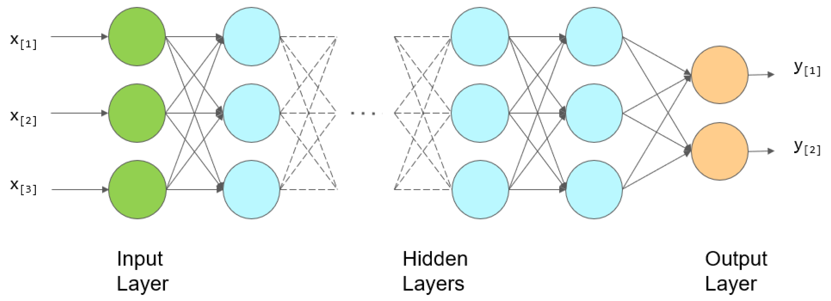
2.1. Artificial Neural Networks

Artificial Neural Network (ANN) is a research hotspot in the field of artificial intelligence since the 1980s [38,39]. It abstracts the human brain neurons from the perspective of information processing and models various networks according to different connections. Specifically, the artificial neural network is used to simulate the process of transmitting information from neuron cells in the brain. It consists of multiple connected artificial neurons and can be used to mine and fit complex relationships hidden within the data. Besides, the connections between different neurons are given different weights, each representing the amount of influence of one neuron on another neuron. Figure 1 illustrates the structure of a feedforward neural network (FNN). Feedforward neural network [40] is a simple artificial neural network in the field of artificial intelligence. As can be seen in Figure 1, a feedforward neural network consists of an input layer, one or more hidden layers, and an output layer. Within it, parameters are propagated from the input layer through the hidden layer to the output layer. When designing a neural network, the number of hidden layers, the number of neurons per layer, and the selection of activation functions are all important factors to consider.

As the number of hidden layers increases, an artificial neuron network can be viewed as an adaptive nonlinear dynamic system that consists of a large number of neurons through various connections, which can be used to approximate a variety of complex functions. Although the structure of artificial neural networks is relatively simple, it is not easy to make artificial neural networks capable of learning. It was not until around 1980 that the backpropagation algorithm effectively solved the learning problem of multilayer neural networks, and became the most popular neural network learning algorithm [39,41]. Because an artificial neural network can be used as a function approximator, it can be considered as a learnable function and applied to solve partial differential equations. Theoretically, with enough training data and neurons, artificial neural networks can learn solutions to partial differential equations.

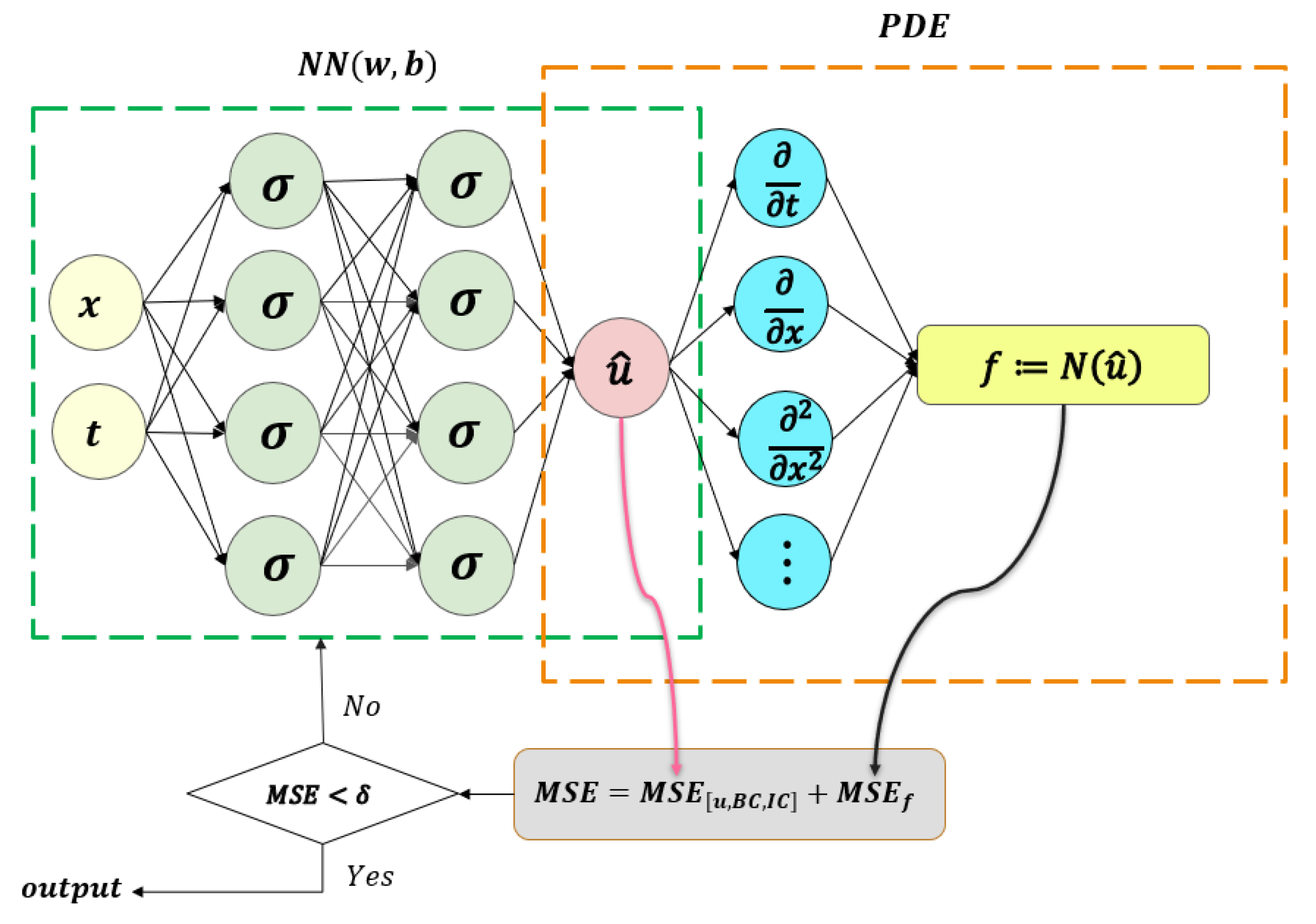
2.2. Physics-Informed Neural Networks

In this section, we introduce the physics-informed neural networks (PINNs) and related settings in this study. Traditional neural networks are based entirely on a data-driven approach that does not take into account the physical laws that are contained in the data. Therefore, a large amount of data is often required to train the neural networks to obtain a reasonable model. In contrast, physics-informed neural networks introduce physical information into the network by forcing the network output to satisfy the corresponding partial differential equations. Specifically, by adding regularization about partial differential equations to the loss function, the model is made to consider physical laws during the training process. This processing makes the training process require less data and speeds up the training process. Physics-informed neural networks can be used to solve not only the forward problem, i.e., obtaining approximate solutions to partial differential equations, but also the inverse problem, i.e., obtaining the parameters of partial differential equations from training data [29,36,42,43]. In the following, the physical-informed neural network modified and used in this study is introduced for the forward problem of partial differential equations.

In this study, consider the partial differential equation defined on the domain $\Omega$ with the boundary $\partial \Omega$.

$$\begin{array}{cc}\mathcal{D}\left(\mathit{u}\right(\mathit{x}\left)\right)=\mathit{0}& \mathit{x}\in \Omega \end{array}$$

(1)

$$\begin{array}{cc}\mathcal{B}\left(\mathit{u}\right(\mathit{x}\left)\right)=\mathit{0}& \mathit{x}\in \partial \Omega \end{array}$$

(2)

where $\mathit{u}$ is the unknown solution and $\mathcal{D}$ denotes a linear or nonlinear differential operator $(e.g.,\partial /\partial \mathit{x},\mathit{u}\circ \partial /\partial \mathit{x},\mathit{u}\circ {\partial }^2/\partial {\mathit{x}}^{\mathbf{2}},etc.)$, and the operator $\mathcal{B}$ denotes the boundary condition of a partial differential Equation (e.g., Dirichlet boundary condition, Neumann boundary condition, Robin boundary condition, etc.). A point to note is that, for partial differential equations that contain temporal variables, we treat t as a special component of $\mathit{x}$, i.e., the temporal domain is included in $\Omega$. At this point, the initial condition can be treated as a special type of Dirichlet boundary condition on the spatio-temporal domain.

First, we construct a neural network for approximating the solution $u\left(\mathit{x}\right)$ of a partial differential equation. This neural network is denoted by $\widehat{u}(\mathit{x};\theta )$, which takes the $\mathit{x}$ as input and outputs a vector of the same dimension as $u\left(\mathit{x}\right)$. Suppose this neural network contains an input layer, $L-1$ hidden layers and an output layer. Specifically, each hidden layer in the neural network receives the output from the previous layer and, in the $k^{th}$ hidden layer, there are $N_k$ number of neurons. $\theta$ is used to represent the neural network parameters, containing the collection of weight matrix $W^{\left[k\right]}\in {\mathit{R}}^{n_k\times n_{k-1}}$ and bias vector $b^{\left[k\right]}\in {\mathit{R}}^{n_k}$ for each layer k with $n_k$ neurons. These parameters will be continuously optimized during the training phase. The neural network $\widehat{u}$ should satisfy two requirements: on the one hand, given a dataset of $u\left(\mathit{x}\right)$ observations, the network should be able to reproduce the observations when $\mathit{x}$ is used as input and, on the other hand, $\widehat{u}$ should conform to the physics underlying the partial differential equation. Thus, we next fulfill the requirements of the second part by defining a residual network.

$$f(\mathit{x};\theta ):=\mathcal{N}\left[\widehat{u}(\mathit{x};\theta )\right]$$

(3)

To build this neural network, we need to use automatic differentiation (AD). Currently, automatic differentiation techniques have been widely integrated into many deep learning frameworks, such as Tensorflow [44] and PyTorch [45]. Therefore, many researchers have commonly used automatic differentiation in their studies of PINNs [29]. In this study, for the surrogate network $\widehat{u}$, we derive the neural network by the automatic differentiation according to the chain rule. Moreover, since the network f has the same parameters as the network $\widehat{u}$, both networks are trained by minimizing a loss function. Specifically, Figure 2 shows a schematic diagram of a physics-informed neural network. The next main task is to find the best neural network parameters that minimize the defined loss function. In a physics-informed neural network, the loss function is defined, as follows

$$J\left(\theta \right)=MS{E}_u+MS{E}_f$$

(4)

The calculation of the mean square error (MSE) is given by the following formula:

$$MS{E}_u=\frac{1}{N_u}\sum _{i=1}^{N_u}{\left|{\widehat{u}}^i-u\left(x_u^i,t_u^i\right)\right|}^2$$

(5)

$$MS{E}_f=\frac{1}{N_f}\sum _{i=1}^{N_f}{\left|f\left(x_f^i,t_f^i\right)\right|}^2$$

(6)

Here, $u\left(x_u^i,t_u^i\right)$ denotes training data from initial and boundary conditions and $u\left(x_f^i,t_f^i\right)$ denotes the training data in the space-time domain. Equation (5) requires the neural network to satisfy the initial and boundary conditions, while Equation (6) requires the neural network to satisfy the constraints of the partial differential equation, which corresponds to the physical information part of the neural network. Next, the optimization problem for Equation (4) is addressed by optimizing the parameters in order to find the minimum value of the loss function, i.e., we seek the following parameters.

$$w^{*}=\underset{w\in \theta }{argmin}\left(J\left(w\right)\right)$$

(7)

$$b^{*}=\underset{b\in \theta }{argmin}\left(J\left(b\right)\right)$$

(8)

In the last step, we use gradient-based optimizers to minimize the loss function, such as SGD, RMSprop, Adam, and L-BFGS [46,47,48]. It is found that, for smooth PDE solutions, L-BFGS can find a good solution faster than Adam, using fewer iterations. This is because Adam optimizer relies only on the first order derivative, whereas L-BFGS uses the second order derivative of the loss function [49]. However, one problem with L-BFGS is that it is more likely to get stuck on a bad local minimum. Considering their respective advantages, in this study we end up using a combination of L-BFGS and Adam optimizer to minimize the loss function. Besides, we also use a residual-based adaptive refinement (RAR) [50] method to improve the training effect by increasing the number of residual points in regions with large residuals of partial differential equations until the residuals are less than the threshold. By the above method, we will obtain trained neural networks that can be used to approximate the solutions of partial differential equations. In the next part, we will use the above method to study three important partial differential equations: the one-dimensional wave equation, the KdV–Burgers equation and the KdV equation.

3. Experiments and Results

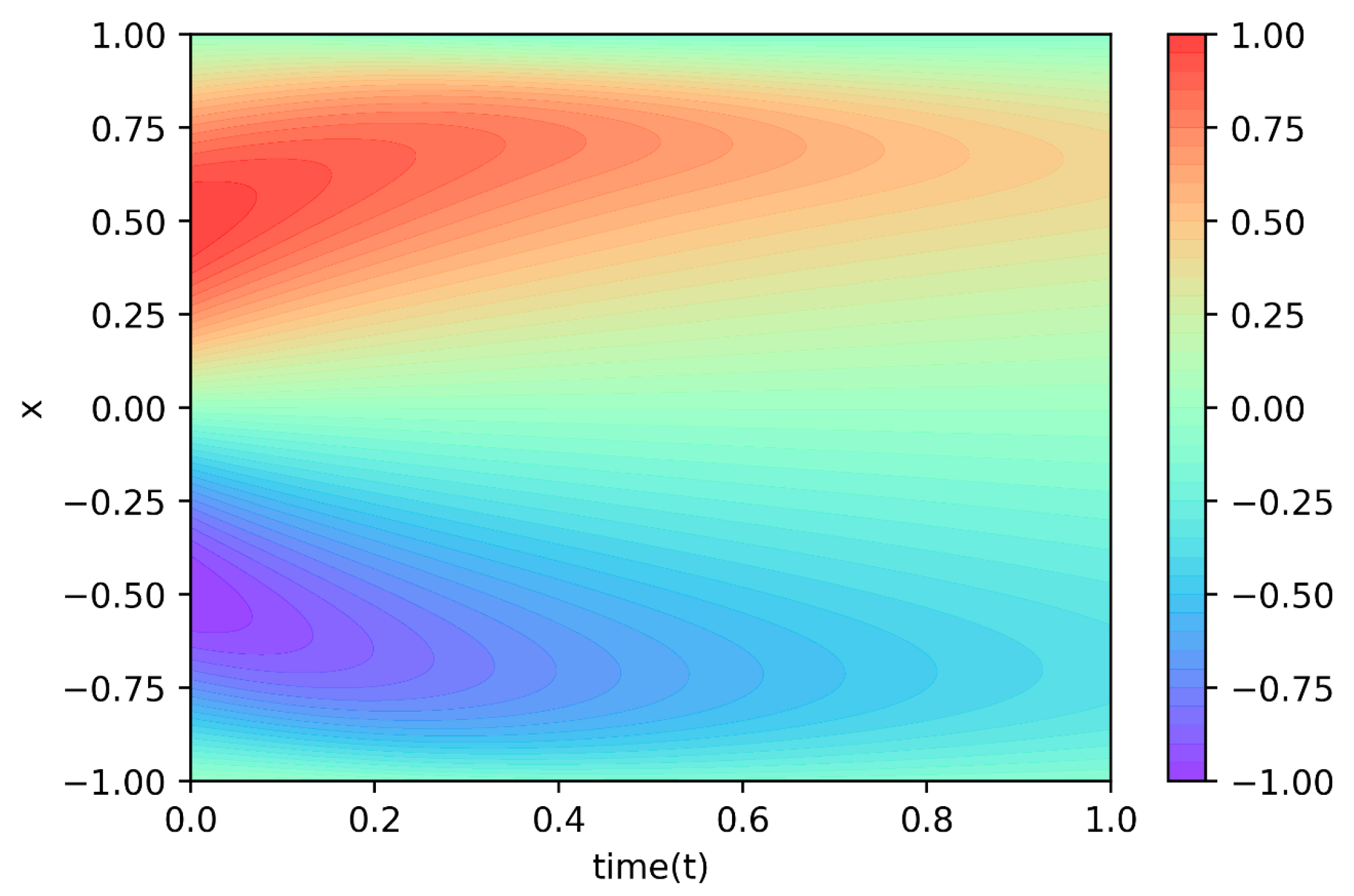
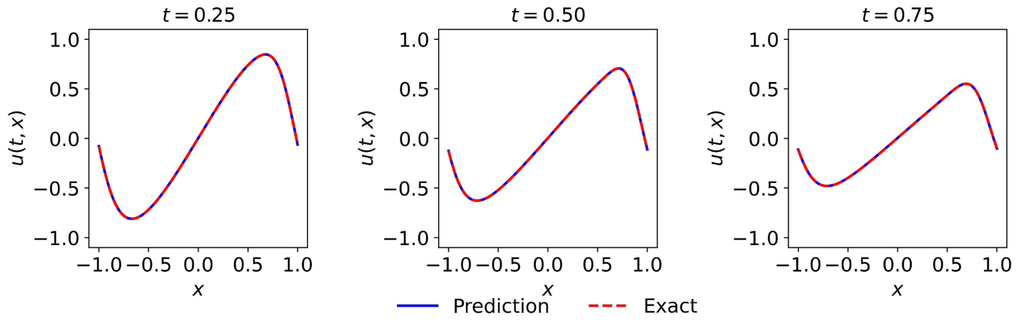
In this section, we study the one-dimensional wave equation, the KdV-Burgers equation and the KdV equation using physics-informed neural networks. The neural network models are constructed for these three equations, respectively, based on the given initial and boundary conditions. The approximation results of the neural networks are compared with the true solutions to test the physics-informed neural networks in this paper. All of the experiments were done on Ubuntu 16.04 and we used the open-source TensorFlow to build and train the neural network models. Besides, we used PyCharm 2019.3 which is developed by JetBrains as the development environment for the experiments and NVIDIA GeForce GTX 1080 Ti. In the following, we will present the experimental design and results of these three equations, respectively.

3.1. Wave Equation

This section presents an experimental study of the wave equation using the physics-informed neural network. The wave equation is a typical hyperbolic partial differential equation and it contains second-order partial derivatives about the independent variable. In physics, the wave equation describes the path of a wave propagating through a medium and is used to study the various types of wave propagation phenomena. It appears in many fields of science, such as acoustic wave propagations, radio communications, and seismic wave propagation [51,52,53]. The study of wave equations is of great importance, as they are widely used in many fields. In this study, we choose a one-dimensional wave equation [54] for our experiments. In mathematical form, this wave equation is defined, as follows:

$$\begin{array}{c}{u}_{tt}-c{u}_{xx}=0,x\in [0,1],t\in [0,1]\hfill \end{array}$$

(9)

where u is a function of the spatial variables x and time t. In the equation, the value of c represents the wave propagation velocity, which is given as 1 in this study. Besides, for this wave equation, its initial conditions and the homogeneous Dirichlet boundary conditions are given, as follows:

$$\begin{array}{c}u(0,x)=\frac{1}{2}sin\left(\pi x\right)\hfill \\ u_t(0,x)=\pi sin\left(3\pi x\right)\hfill \\ u(t,0)=u(t,1)=0\hfill \end{array}$$

(10)

The true solution of the above equation is $u(t,x)=\frac{1}{2}sin\left(\pi x\right)cos\left(\pi t\right)+\frac{1}{3}sin\left(3\pi x\right)sin\left(3\pi t\right)$, which we use to generate the data. The initial conditions, boundary conditions, and some random data in the space-time domain are used as training data to train the neural network model. In order to test the performance of the training model, we use the neural network model to make multiple predictions and compare it with the true solution of the partial differential equation. The specific experimental setup and procedure are as follows.

First, a neural network is designed for approximating the solutions of partial differential equations, denoted as $\widehat{u}(t,x)$. For the architecture of the neural network, it contains six hidden layers, each with 100 neurons, and a hyperbolic tangent tanh is chosen as the activation function. Besides, a physics-informed neural network $f(t,x)$ is constructed for introducing control information of the equation. In our experiments, we use TensorFlow to construct the neural network. As a widely used deep learning framework, it has sophisticated automatic differentiation, so it is easy to introduce information about the equations. Specifically, the definition of a physical information neural network $f(t,x)$ is given by

$$f(t,x):=u_{tt}-u_{xx}$$

(11)

The next main task is to train the parameters of the neural network $\widehat{u}(t,x)$ and $f(t,x)$. We continuously optimize the parameters by minimizing the mean square error loss to obtain the optimal parameters.

$$J\left(\theta \right)=MS{E}_u+MS{E}_f$$

(12)

where

$$MS{E}_u=\frac{1}{N_u}\sum _{i=1}^{N_u}{\left|u\left(t_u^i,x_u^i\right)-u^i\right|}^2$$

(13)

$$MS{E}_f=\frac{1}{N_f}\sum _{i=1}^{N_f}{\left|f\left(t_f^i,x_f^i\right)\right|}^2$$

(14)

where $MS{E}_u$ is a loss function constructed using observations of initial and boundary conditions. $MS{E}_f$ is a loss function that is based on partial differential equations for introducing physical information. Specifically, ${\left\{t_u^i,x_u^i,u^i\right\}}_{i=1}^{N_u}$ corresponds to the initial and boundary training data of $u(t,x)$, and $N_u$ is the number of data provided. In addition, $u(t_f,x_f)$ and ${\left\{t_f^i,x_f^i\right\}}_{i=1}^{N_f}$ corresponds to the training data of the spatio-temporal domain, and $N_f$ is the corresponding number of training data. In this work, to fully consider the physical information embedded in the equations, we select the data in the spatio-temporal domain to train the neural network. The training data of the spatio-temporal domain is selected randomly, and the amount of training data $N_f$ is 40,000. Besides, the total number of training data of the initial and boundary conditions is relatively small, and the expected effect can be achieved when $N_u$ is 300. Similarly, the selection of training data for the initial and boundary conditions is also random. During the optimization procedure, we set the learning rate to 0.001, and in order to balance convergence speed and global convergence, we ran L-BFGS 30,000 epochs and then continued the optimization using Adam until convergence. In addition, we used the Glorot normal initializer [55] for initialization. In this experiment, the time to train the model was approximately fifteen minutes. We tested the effect of the model after completing the training of the neural network model. Figure 3 is the prediction of the neural network model obtained from the training, and it can be seen that the prediction obtained is quite complex. We choose different moments to compare the prediction with the exact solution to test the accuracy of this prediction. Figure 4 shows the comparison between the exact solution and the prediction at different times $t=0.2,0.5,0.8$. From Figure 4, it can be seen that the predictions of the neural network model and exact solutions are very consistent, indicating that the constructed neural network model has a good ability to solve partial differential equations. In addition, the relative L2 error of this example was calculated to be $5.16·{10}^{-4}$, which further validates the effectiveness of this method. Although the solution of the selected partial differential equations is complex, the neural network model can still approximate a result very close to the true solution from the training data, indicating that the neural network with physical information has great potential and value, and is worthy of further research.

3.2. KdV-Burgers Equation

We have studied the KdV–Burgers equation to further analyze the ability of physics-informed neural networks to solve complex partial differential equations. The KdV–Burgers equation is a nonlinear partial differential equation containing higher-order derivatives that has been of interest to many researchers [56,57]. Today, the KdV–Burgers equation is widely studied and applied in many fields, such as the study of the flow of liquids containing bubbles, the flow of liquids in elastic tubes, and other problems [58,59]. In mathematical form, the KdV–Burgers equation is defined, as follows:

$$u_t+\alpha u{u}_x+\beta u_{xx}+\gamma u_{xxx}=0$$

(15)

where $\alpha$, $\beta$ and $\gamma$ are all non-zero real constants, i.e., $\alpha \beta \gamma \ne 0$. Equation (15) can be reduced to Burgers equation [60] or Korteweg-de Vries (KdV) equation [61] in special cases. Specifically, when $\gamma =0$, the Equation (15) is simplified to Burgers equation.

$$u_t+\alpha u{u}_x+\beta u_{xx}=0$$

(16)

The Burgers equation is a second-order nonlinear partial differential equation, which is used to simulate the propagation and reflection of shock waves. This equation is used in various fields of research, such as fluid dynamics and nonlinear acoustics (NLA) [60,62]. Besides, Equation (15) becomes the Korteweg-de Vries (KdV) equation when $\beta$ is zero.

$$u_t+\alpha u{u}_x+\gamma u_{xxx}=0$$

(17)

The Korteweg-de Vries (KdV) equation was first introduced in 1985 by Korteweg and de Vries. It is a very important equation, both mathematically and practically, for the description of small amplitude shallow-water waves, ion-phonon waves, and fluctuation phenomena in biological and physical systems [63,64]. This equation, which differs from the Burgers equation in that it does not introduce dissipation and it can explain the existence of solitary waves, is of great interest to physicists and mathematicians. Therefore, the study of this equation is of great scientific significance and research value.

The KdV–Burgers equation can be viewed as a combination of the Korteweg-de Vries equation and the Burgers equation, containing the nonlinearity $u{u}_x$, the dispersion $u_{xxx}$, and the dissipation $u_{xx}$, with high complexity. The equation has been applied in many fields and it has received a great deal of attention from many researchers. In this section, we use physics-informed neural networks to develop new methods for solving the KdV–Burgers equation.

In this experiment, an important task is to construct a high-quality training data set based on partial differential equations. For Equation (15), the values of $\alpha ,\beta ,\gamma$ are given as 1,−0.075,$\pi /1000$, respectively, and deterministic initial conditions are given. In mathematical form, the nonlinear KdV–Burgers equation with periodic boundary conditions studied in this section is defined, as follows

$$\begin{array}{c}{u}_t+u{u}_x-0.075u_{xx}+\pi /1000u_{xxx}=0,x\in [-1,1],t\in [0,1]\hfill \\ u(0,x)=e^{(0.005*cos(\pi *x\left)\right)}sin(\pi *x)\hfill \\ u(t,-1)=u(t,1)\hfill \\ u_x(t,-1)=u_x(t,1)\hfill \end{array}$$

(18)

For Equation (18), we simulate it using conventional spectral methods and use the Chebfun package [65] in the programming implementation. Specifically, we integrate Equation (18) from the initial moment $t=0$ to the final time $t=1.0$ using a time step $t={10}^{-6}$, depending on the initial and periodic boundary conditions. Besides, we use a fourth-order explicit Runge–Kutta temporal integrator and a spectral Fourier discretization with 512 modes to ensure the accuracy of the integration.

After obtaining the high-resolution dataset, we next constructed a neural network to approximate the solution of Equation (18), which is denoted as $\widehat{u}(t,x)$. The neural network contains seven hidden layers, each containing 120 neurons, and the hyperbolic tangent tanh is chosen as the activation function. Besides, the physical information neural network $f(t,x)$ is constructed using the automatic differentiation of the TensorFlow to introduce control information of the equations. Specifically, the physics-informed neural network $f(t,x)$ is defined, as follows

$$f(t,x):=u_t+u{u}_x-0.075u_{xx}+\pi /1000u_{xxx}$$

(19)

The next main task is to train the parameters of the neural network $\widehat{u}(t,x)$ and $f(t,x)$. We continuously optimize the parameters by minimizing the mean square error loss to obtain the optimal parameters.

$$J\left(\theta \right)=MS{E}_u+MS{E}_f$$

(20)

where

$$MS{E}_u=\frac{1}{N_u}\sum _{i=1}^{N_u}{\left|u\left(t_u^i,x_u^i\right)-u^i\right|}^2$$

(21)

$$MS{E}_f=\frac{1}{N_f}\sum _{i=1}^{N_f}{\left|f\left(t_f^i,x_f^i\right)\right|}^2$$

(22)

Similar to the previous experiment, $MS{E}_u$ is a loss function constructed while using observations of the initial and boundary conditions. $MS{E}_f$ is a loss function that introduces physical information of partial differential equations. Specifically, ${\left\{t_u^i,x_u^i,u^i\right\}}_{i=1}^{N_u}$ corresponds to the initial and boundary condition data, $u(t_f,x_f)$ and ${\left\{t_f^i,x_f^i\right\}}_{i=1}^{N_f}$ corresponds to the data in the space-time domain. In this experiment, the training data are also randomly selected from the generated dataset, with the number of training data $N_f$ in the space-time domain being 30,000 and the number of training data $N_u$ in the initial and boundary conditions being 400. We use the Glorot normal initializer for initialization. During optimization, we set the learning rate to 0.001 and, to ensure global convergence and speed up the convergence process, we ran L-BFGS for 30,000 epochs and then used Adam to continue optimizing until convergence. In this experiment, the time to train the model was approximately twelve minutes. After completing the training of the neural network model, we also tested the effects of the model. Figure 5 shows the predictions of the neural network model, and we can see that the resulting predictions are quite complex. We choose different moments of the prediction results to compare with the exact solution in order to test the accuracy of this prediction. Figure 6 shows the comparison between the exact solution and prediction at different moments $t=0.25,0.5,0.75$. From Figure 6, it can be seen that the predictions of the neural network model and exact solutions are highly consistent, indicating that the constructed neural network model can solve the KdV–Burgers equation well. In addition, the relative L2 error of this example was calculated to be $4.79·{10}^{-4}$, which further validates the effectiveness of this method. Despite the high complexity of the KdV–Burgers equation, the neural network model can still obtain results very close to the true solution from the training data, which again shows that the method has great potential and value and it is worthy of further research.

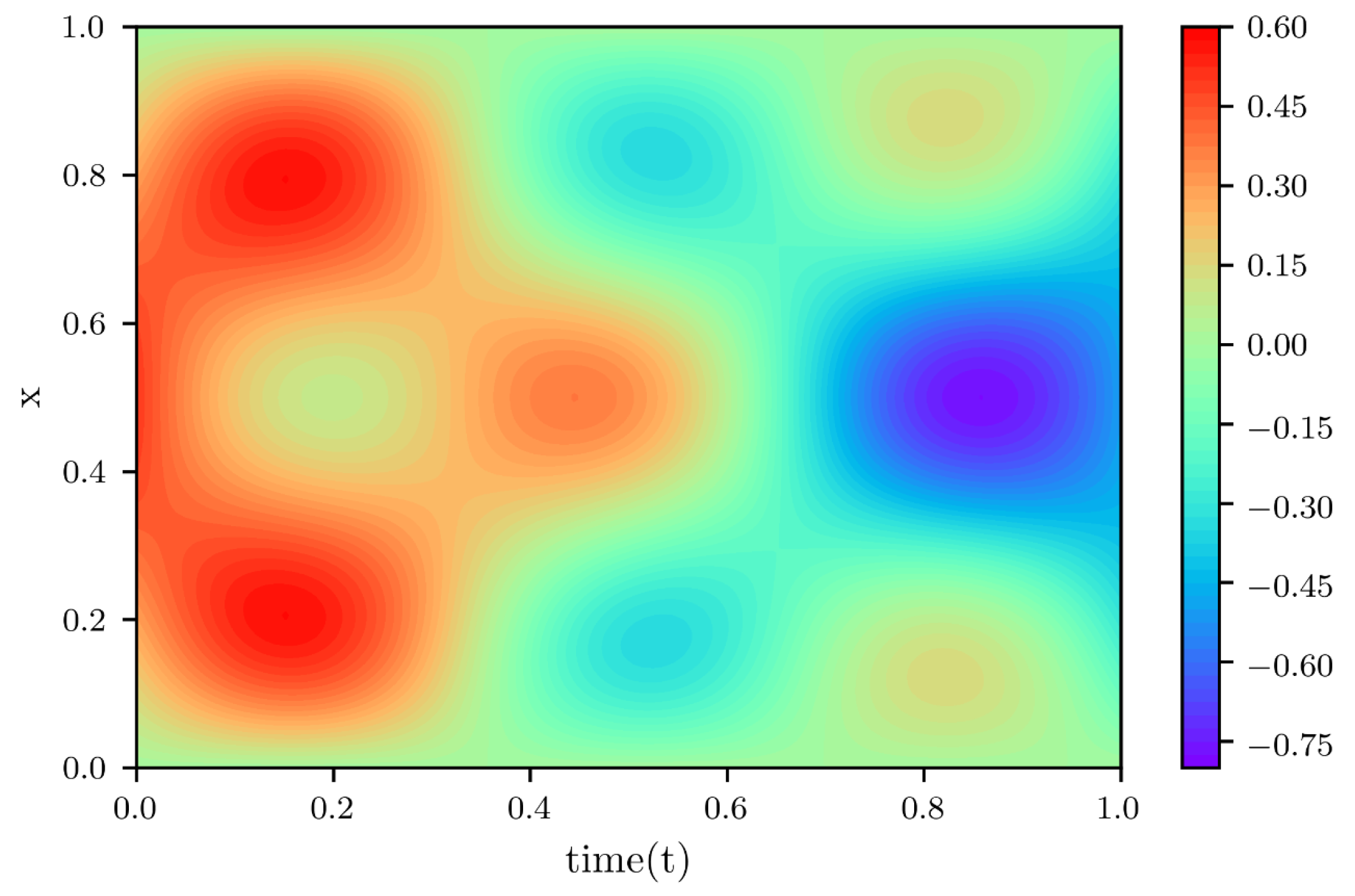
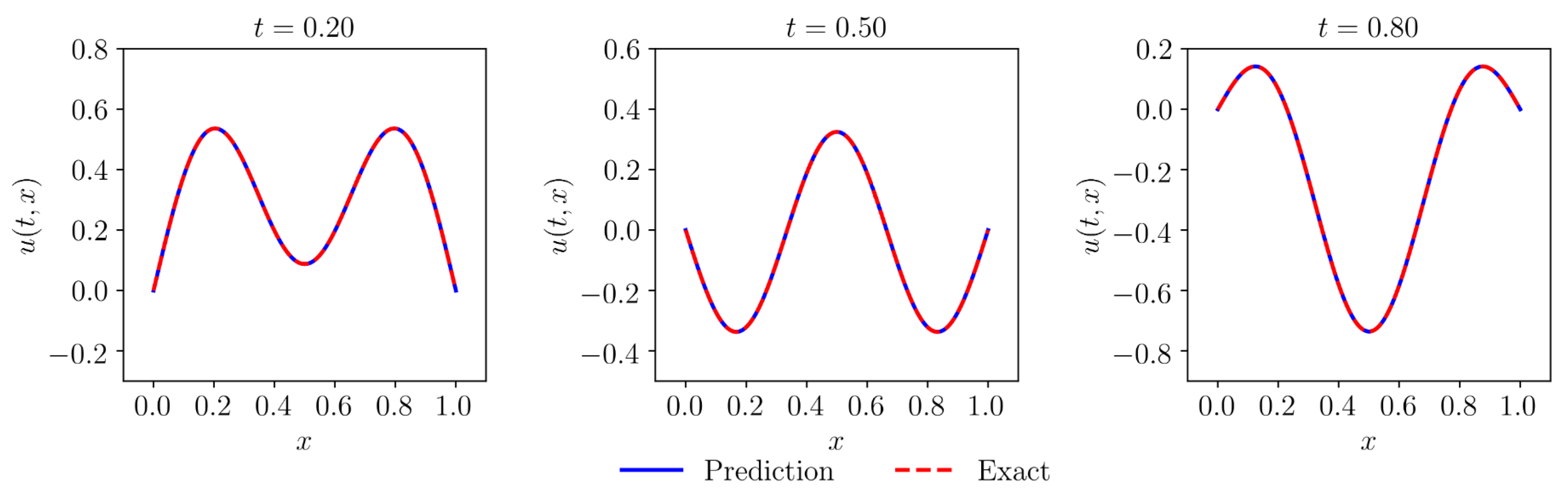
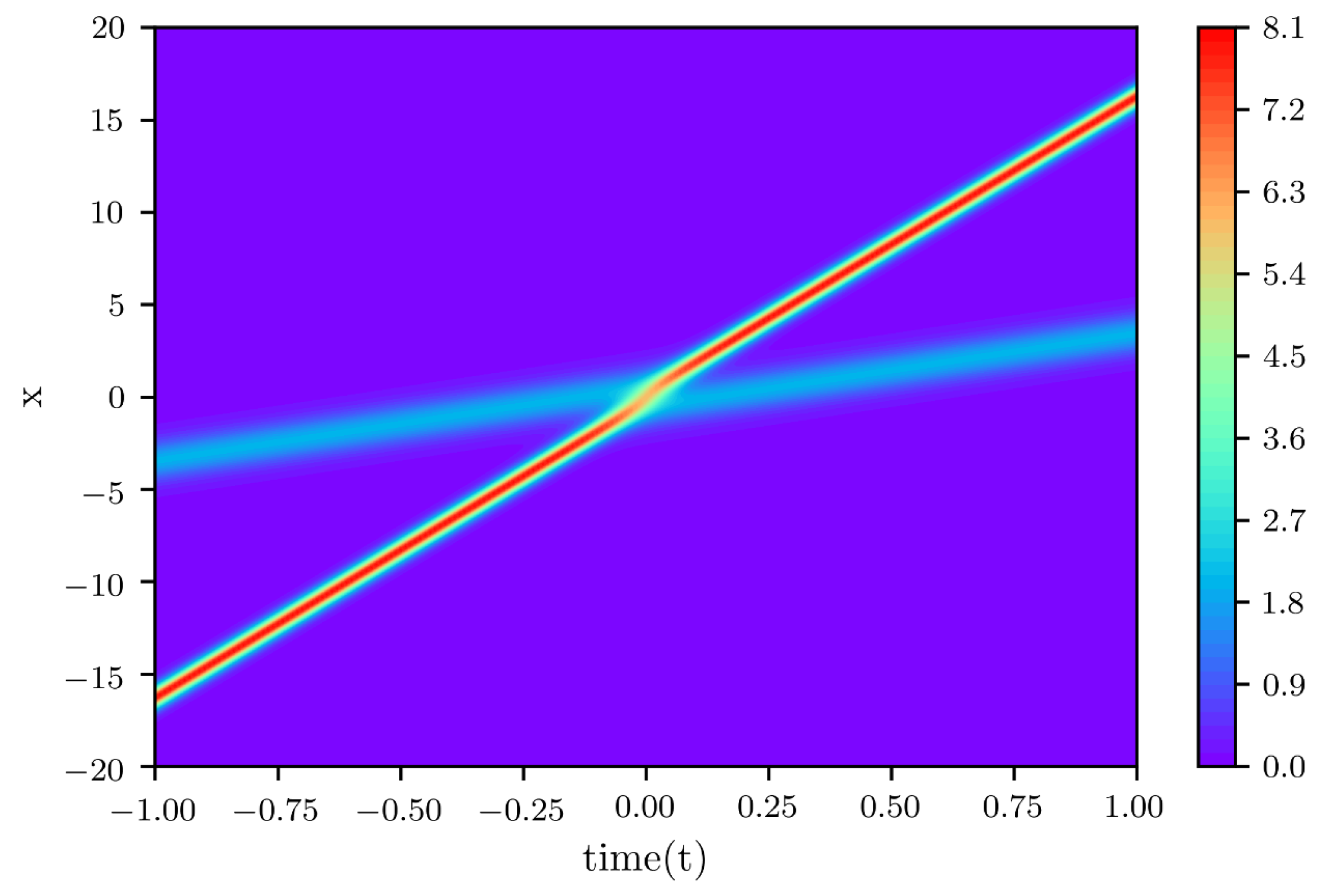
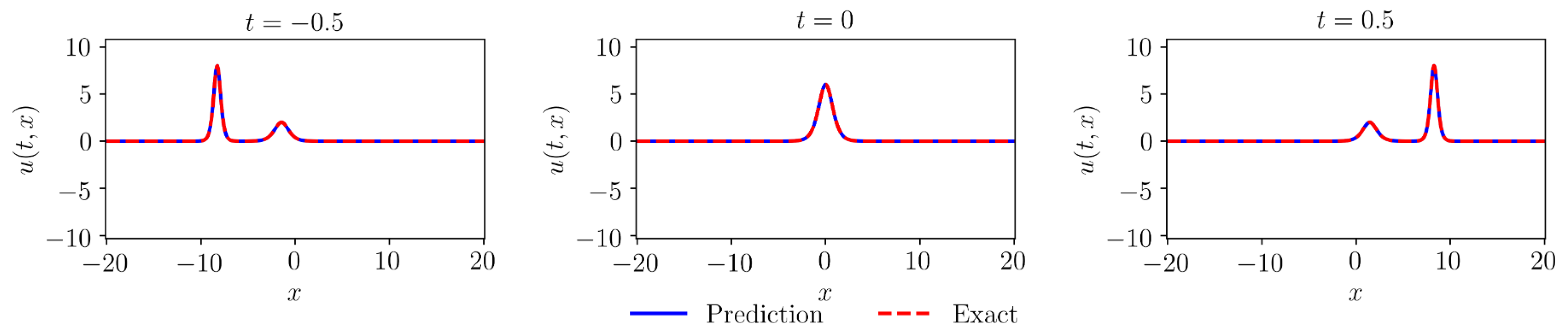
3.3. Two-Soliton Solution of the Korteweg-De Vries Equation

KdV equations are an important class of equations that have soliton solutions, as introduced in Section 3.2. The study of the KdV equation is important for understanding the nature of solitons and the interaction of two or more solitons. Many scholars have studied the multi-soliton solutions of KdV equations [66] and, in this section, we employ the proposed physics-informed neural networks to study the following KdV equations:

$$\begin{array}{c}{u}_t+6u{u}_x+u_{xxx}=0,-\infty <x<\infty \hfill \end{array}$$

(23)

when given the initial condition $u(0,x)=6sec{h}^{2}x$, Equation (23) has the following two-soliton solution $u(x,t)$

$$\begin{array}{c}u(x,t)=12\frac{3+4cosh(2x-8t)+cosh(4x-64t)}{{(3cosh(x-28t)+cosh(3x-36t))}^2}\hfill \end{array}$$

(24)

First, because this solution is valid for either positive or negative t, we obtained data based on the true solution for $x\in [-20,20]$ and $t\in [-1,1]$. Some initial data and some random data in the space-time domain are selected as training data. Next, we constructed a neural network to approximate the solution of Equation (23), which is denoted as $\widehat{u}(t,x)$. The neural network contains seven hidden layers, each containing 100 neurons, and the hyperbolic tangent tanh is chosen as the activation function. Besides, the physical information neural network $f(t,x)$ is constructed using the automatic differentiation of the TensorFlow in order to introduce control information of the equation. Specifically, the physics-informed neural network $f(t,x)$ is defined, as follows:

$$f(t,x):=u_t+6u{u}_x+u_{xxx}$$

(25)

Next, we obtain the optimal parameters of the neural network $\widehat{u}(t,x)$ and $f(t,x)$ by minimizing the following mean square error loss.

$$J\left(\theta \right)=MS{E}_u+MS{E}_f$$

(26)

where

$$MS{E}_u=\frac{1}{N_u}\sum _{i=1}^{N_u}{\left|u\left(t_u^i,x_u^i\right)-u^i\right|}^2$$

(27)

$$MS{E}_f=\frac{1}{N_f}\sum _{i=1}^{N_f}{\left|f\left(t_f^i,x_f^i\right)\right|}^2$$

(28)

Similar to the previous experiment, on the one hand, the loss function $MS{E}_u$ is constructed based on the observation data of the initial condition and boundary condition; on the other hand, the loss function $MS{E}_f$ is constructed based on the physical information of the partial differential equation. Specifically, ${\left\{t_u^i,x_u^i,u^i\right\}}_{i=1}^{N_u}$ corresponds to the initial and boundary condition data, $u(t_f,x_f)$ and ${\left\{t_f^i,x_f^i\right\}}_{i=1}^{N_f}$ corresponds to the data in the space-time domain. In this experiment, we randomly select training data in the data set. The number of training data in the spatio-temporal domain is 60,000, and the number of training data that meets the initial and boundary conditions is 400. We used the Glorot normal initializer for initialization and set the learning rate for the optimization process to 0.001. We ran L-BFGS for 30,000 epochs and then used Adam to continue the optimization until convergence to ensure global convergence and speed up the convergence process. In this experiment, the time to train the model was about eighteen minutes. After training the neural network model, we used the model to make predictions and compared the results with the true solution. Figure 7 shows the predictions of the KdV equation given by physics-informed neural networks. Figure 8 gives the comparison between the prediction and the exact solution at different moments $t=-0.5,0,0.5$ to test the performance of the model. It can be seen from Figure 8 that the prediction is very close to the exact solution. Also, it can be seen that tall wave propagates faster than short waves, which is consistent with the nature of the solitary wave solutions of the KdV equation. Thus, it can be concluded that the neural network model can simulate the KdV equation well. Besides, the relative L2 error was calculated to be $4.62·{10}^{-3}$ in this case, further validating the effectiveness of the method. Because physics-informed neural networks can simulate the solitary wave solution of the KdV equation well, we will apply this method to the study of multi-soliton solutions of other equations, such as the Boussinesq equation [66,67], in future studies.

4. Discussions

In this study, three partial differential equations are investigated using physics-informed neural networks. Based on the characteristics of the wave equation, the KdV-Burgers equation, and the KdV equation, the corresponding neural network models were constructed and each model was experimentally analyzed. We compare the predictions of the physics-informed neural network with the true solutions of the equations and derive the following discussion.

(1)

The most important task of physics-informed neural networks is to introduce a reasonable regularization of physical information. The use of physical information allows neural networks to better learn the solutions of partial differential equations from fewer observations. In this study, the physical information regularization is implemented through the automatic differentiation of the TensorFlow framework, which may not be applicable in many practical problems. Therefore, we need to develop more general differential methods and expand more methods for introducing physical information so that physics-informed neural networks can be better applied to real-world problems.

(2)

Regularization has an important role in physics-informed neural networks. Similar to the previous related studies, the regularization in this study takes the form of the L2 norm. However, when considering the advantages of different norms, such as the ability of L1 norm to resist anomalous data interference, in the next study, we will adopt different forms of regularization of physical information such as L1 norm, to further improve the theory and methods related to physics-informed neural networks.

(3)

In this study, the training data used to train the physics-informed neural network are randomly selected in the space-time domain, thus the physics-informed neural network does not need to consider the discretization of partial differential equations and can learn the solutions of partial differential equations from a small amount of data. It is well known that popular computational fluid dynamics methods require consideration of the discretization of equations, such as finite difference methods. In practice, many engineering applications also need to consider the discretization of partial differential equations, for example, various numerical weather prediction models have made discretization schemes as an important part of their research. Physics-informed neural networks are well suited to solve this problem and, thus, this approach may have important implications for the development of computational fluid dynamics and even scientific computing.

(4)

Although the method used in this paper has many advantages, such as not having to consider the discretization of PDEs. However, the method also faces many problems, such as the neural network for solving PDEs relies heavily on training data, which often requires more training time when the quality of the training data is poor. Therefore, it is also important to investigate how to construct high-quality training datasets to reduce the training time.

(5)

In this study, we focus on solving PDEs by training physics-informed neural networks, which is a supervised learning task. Currently, several researchers have used unlabeled data to train physics-constrained deep learning models for high-dimensional problems and have quantified the uncertainty of the predictions [68]. This inspires us to further improve our neural network, so that it can be trained using unlabeled data and give a probabilistic interpretation of the prediction results [69]. Besides, this paper studies low-dimensional problems, whereas, for high-dimensional problems, model reduction [70] is also an important issue to consider when constructing a neural network model.

(6)

In this paper, we study one-dimensional partial differential equations, but the method can be applied to multi-dimensional problems. Currently, we are attempting to apply the method to the simulation of three-dimensional atmospheric equations for improving existing numerical weather prediction models. Besides, in the field of engineering, complex PDE systems of field coupled nature, as in Fluid-Structure Interaction, are of great research value and they are widely used in the aerospace industry, nuclear engineering, etc. [71], so we will also study such complex PDEs in the future.

(7)

So far, there have been many promising applications of neural networks in computational engineering. For example, one very interesting work is that neural networks have been used to construct constitutive laws as a surrogate model replacing the two-scale computational approaches [72,73]. These valuable works will guide us in further exploring the applications of neural networks in scientific computing.

5. Conclusions

This paper introduces a method for solving partial differential equations by neural networks that fuse physical information. The method is an improvement on previous physics-informed neural networks. In this study, the physical laws that are contained in the partial differential equations are introduced into the neural networks as a regularization. This improvement motivates the neural network to better learn the solutions of the partial differential equations from a limited number of observations. Using the method presented in this paper, we have performed the experimental analysis of three important partial differential equations. The method proposed in this paper achieves good experimental results due to the powerful function approximation ability of neural networks and the physical information contained in the partial differential equations. It is believed that, in the future, physics-informed neural networks will profoundly influence the study of solving partial differential equations and even promote the development of the whole field of scientific computing. However, there are still many problems with physics-informed neural networks, such as how to better introduce physical information into neural networks and the possible non-convergence problem in loss function optimization, which is also the next focus of our research. Besides, in the future, we will focus on analyzing the performance differences between PINN-based methods and FEM methods, comparing their accuracy, consumption time, and so on.

References

1. Folland, G.B. Introduction to Partial Differential Equations; Princeton University Press: Princeton, NJ, USA, 1995; Volume 102. [Google Scholar]
2. Petrovsky, I.G. Lectures on Partial Differential Equations; Courier Corporation: North Chelmsford, MA, USA, 2012. [Google Scholar]
3. Courant, R.; Hilbert, D. Methods of Mathematical Physics: Partial Differential Equations; John Wiley & Sons: Hoboken, NJ, USA, 2008. [Google Scholar]
4. Farlow, S.J. Partial Differential Equations for Scientists and Engineers; Courier Corporation: North Chelmsford, MA, USA, 1993. [Google Scholar]
5. Zauderer, E. Partial Differential Equations of Applied Mathematics; John Wiley & Sons: Hoboken, NJ, USA, 2011; Volume 71. [Google Scholar]
6. Churchfield, M.J.; Lee, S.; Michalakes, J.; Moriarty, P.J. A numerical study of the effects of atmospheric and wake turbulence on wind turbine dynamics. J. Turbul. 2012, 13, N14. [Google Scholar] [CrossRef]
7. Müller, E.H.; Scheichl, R. Massively parallel solvers for elliptic partial differential equations in numerical weather and climate prediction. Q. J. R. Meteorol. Soc. 2014, 140, 2608–2624. [Google Scholar] [CrossRef] [Green Version]
8. Tröltzsch, F. Optimal Control of Partial Differential Equations: Theory, Methods, and Applications; American Mathematical Society: Providence, RI, USA, 2010; Volume 112. [Google Scholar]
9. Ames, W.F. Numerical Methods for Partial Differential Equations; Academic Press: Cambridge, MA, USA, 2014. [Google Scholar]
10. Quarteroni, A.; Valli, A. Numerical Approximation of Partial Differential Equations; Springer: Berlin/Heidelberg, Germany, 2008; Volume 23. [Google Scholar]
11. Yin, S.; Ding, S.X.; Xie, X.; Luo, H. A review on basic data-driven approaches for industrial process monitoring. IEEE Trans. Ind. Electron. 2014, 61, 6418–6428. [Google Scholar] [CrossRef]
12. Bai, Z.; Brunton, S.L.; Brunton, B.W.; Kutz, J.N.; Kaiser, E.; Spohn, A.; Noack, B.R. Data-driven methods in fluid dynamics: Sparse classification from experimental data. In Whither Turbulence and Big Data in the 21st Century? Springer: Berlin/Heidelberg, Germany, 2017; pp. 323–342. [Google Scholar]
13. Goodfellow, I.; Bengio, Y.; Courville, A. Deep Learning; MIT Press: Cambridge, MA, USA, 2016. [Google Scholar]
14. LeCun, Y.; Bengio, Y.; Hinton, G. Deep learning. Nature 2015, 521, 436–444. [Google Scholar] [CrossRef] [PubMed]
15. Deng, L.; Yu, D. Deep learning: Methods and applications. Found. Trends Signal Process. 2014, 7, 197–387. [Google Scholar] [CrossRef] [Green Version]
16. Li, S.; Song, W.; Fang, L.; Chen, Y.; Ghamisi, P.; Benediktsson, J.A. Deep learning for hyperspectral image classification: An overview. IEEE Trans. Geosci. Remote. Sens. 2019, 57, 6690–6709. [Google Scholar] [CrossRef] [Green Version]
17. Goldberg, Y. A primer on neural network models for natural language processing. J. Artif. Intell. Res. 2016, 57, 345–420. [Google Scholar] [CrossRef] [Green Version]
18. Helbing, G.; Ritter, M. Deep Learning for fault detection in wind turbines. Renew. Sustain. Energy Rev. 2018, 98, 189–198. [Google Scholar] [CrossRef]
19. Lu, Y.; Lu, J. A Universal Approximation Theorem of Deep Neural Networks for Expressing Distributions. arXiv 2020, arXiv:2004.08867. [Google Scholar]
20. Hornik, K.; Stinchcombe, M.; White, H. Universal approximation of an unknown mapping and its derivatives using multilayer feedforward networks. Neural Networks 1990, 3, 551–560. [Google Scholar] [CrossRef]
21. Lagaris, I.E.; Likas, A.; Fotiadis, D.I. Artificial neural networks for solving ordinary and partial differential equations. IEEE Trans. Neural Networks 1998, 9, 987–1000. [Google Scholar] [CrossRef] [PubMed] [Green Version]
22. Göküzüm, F.S.; Nguyen, L.T.K.; Keip, M.A. An Artificial Neural Network Based Solution Scheme for Periodic Computational Homogenization of Electrostatic Problems. Math. Comput. Appl. 2019, 24, 40. [Google Scholar] [CrossRef] [Green Version]
23. Nguyen-Thanh, V.M.; Zhuang, X.; Rabczuk, T. A deep energy method for finite deformation hyperelasticity. Eur. J. -Mech.-A/Solids 2020, 80, 103874. [Google Scholar] [CrossRef]
24. Bar, L.; Sochen, N. Unsupervised deep learning algorithm for PDE-based forward and inverse problems. arXiv 2019, arXiv:1904.05417. [Google Scholar]
25. Freund, J.B.; MacArt, J.F.; Sirignano, J. DPM: A deep learning PDE augmentation method (with application to large-eddy simulation). arXiv 2019, arXiv:1911.09145. [Google Scholar]
26. Wu, K.; Xiu, D. Data-driven deep learning of partial differential equations in modal space. J. Comput. Phys. 2020, 408, 109307. [Google Scholar] [CrossRef] [Green Version]
27. Khoo, Y.; Lu, J.; Ying, L. Solving parametric PDE problems with artificial neural networks. arXiv 2017, arXiv:1707.03351. [Google Scholar]
28. Huang, X. Deep neural networks for waves assisted by the Wiener–Hopf method. Proc. R. Soc. 2020, 476, 20190846. [Google Scholar] [CrossRef] [Green Version]
29. Raissi, M.; Perdikaris, P.; Karniadakis, G.E. Physics-informed neural networks: A deep learning framework for solving forward and inverse problems involving nonlinear partial differential equations. J. Comput. Phys. 2019, 378, 686–707. [Google Scholar] [CrossRef]
30. Raissi, M.; Perdikaris, P.; Karniadakis, G.E. Physics Informed Deep Learning (Part I): Data-driven Solutions of Nonlinear Partial Differential Equations. arXiv 2017, arXiv:1711.10561. [Google Scholar]
31. Raissi, M.; Perdikaris, P.; Karniadakis, G.E. Physics Informed Deep Learning (Part II): Data-driven Discovery of Nonlinear Partial Differential Equations. arXiv 2017, arXiv:1711.10566. [Google Scholar]
32. Chen, X.; Duan, J.; Karniadakis, G.E. Learning and meta-learning of stochastic advection-diffusion-reaction systems from sparse measurements. arXiv 2019, arXiv:1910.09098. [Google Scholar]
33. He, Q.; Barajas-Solano, D.; Tartakovsky, G.; Tartakovsky, A.M. Physics-informed neural networks for multiphysics data assimilation with application to subsurface transport. Adv. Water Resour. 2020, 141, 103610. [Google Scholar] [CrossRef]
34. Tartakovsky, A.; Marrero, C.O.; Perdikaris, P.; Tartakovsky, G.; Barajas-Solano, D. Physics-Informed Deep Neural Networks for Learning Parameters and Constitutive Relationships in Subsurface Flow Problems. Water Resour. Res. 2020, 56, e2019WR026731. [Google Scholar] [CrossRef]
35. Kadeethum, T.; Jørgensen, T.M.; Nick, H.M. Physics-informed neural networks for solving nonlinear diffusivity and Biot’s equations. PLoS ONE 2020, 15, e0232683. [Google Scholar] [CrossRef] [PubMed]
36. Kissas, G.; Yang, Y.; Hwuang, E.; Witschey, W.R.; Detre, J.A.; Perdikaris, P. Machine learning in cardiovascular flows modeling: Predicting arterial blood pressure from non-invasive 4D flow MRI data using physics-informed neural networks. Comput. Methods Appl. Mech. Eng. 2020, 358, 112623. [Google Scholar] [CrossRef]
37. Jagtap, A.D.; Kawaguchi, K.; Karniadakis, G.E. Adaptive activation functions accelerate convergence in deep and physics-informed neural networks. J. Comput. Phys. 2020, 404, 109136. [Google Scholar] [CrossRef] [Green Version]
38. Shanmuganathan, S. Artificial neural network modelling: An introduction. In Artificial Neural Network Modelling; Springer: Berlin/Heidelberg, Germany, 2016; pp. 1–14. [Google Scholar]
39. Nielsen, M.A. Neural Networks and Deep Learning; Determination Press: San Francisco, CA, USA, 2015; Volume 2018. [Google Scholar]
40. Svozil, D.; Kvasnicka, V.; Pospichal, J. Introduction to multi-layer feed-forward neural networks. Chemom. Intell. Lab. Syst. 1997, 39, 43–62. [Google Scholar] [CrossRef]
41. Li, J.; Cheng, J.H.; Shi, J.Y.; Huang, F. Brief introduction of back propagation (BP) neural network algorithm and its improvement. In Advances in Computer Science and Information Engineering; Springer: Berlin/Heidelberg, Germany, 2012; pp. 553–558. [Google Scholar]
42. Zhang, D.; Guo, L.; Karniadakis, G.E. Learning in modal space: Solving time-dependent stochastic PDEs using physics-informed neural networks. SIAM J. Sci. Comput. 2020, 42, A639–A665. [Google Scholar] [CrossRef]
43. Tipireddy, R.; Perdikaris, P.; Stinis, P.; Tartakovsky, A. A comparative study of physics-informed neural network models for learning unknown dynamics and constitutive relations. arXiv 2019, arXiv:1904.04058. [Google Scholar]
44. Abadi, M.; Barham, P.; Chen, J.; Chen, Z.; Davis, A.; Dean, J.; Devin, M.; Ghemawat, S.; Irving, G.; Isard, M.; et al. Tensorflow: A system for large-scale machine learning. In Proceedings of the 12th {USENIX} symposium on operating systems design and implementation ({OSDI} 16), Savannah, GA, USA, 2–4 November 2016; pp. 265–283. [Google Scholar]
45. Paszke, A.; Gross, S.; Chintala, S.; Chanan, G.; Yang, E.; DeVito, Z.; Lin, Z.; Desmaison, A.; Antiga, L.; Lerer, A. Automatic differentiation in pytorch. In Proceedings of the NIPS 2017 Autodiff Workshop, Long Beach, CA, USA, 9 December 2017. [Google Scholar]
46. Bengio, Y. Gradient-based optimization of hyperparameters. Neural Comput. 2000, 12, 1889–1900. [Google Scholar] [CrossRef] [PubMed]
47. Kylasa, S.; Roosta, F.; Mahoney, M.W.; Grama, A. GPU accelerated sub-sampled newton’s method for convex classification problems. In Proceedings of the 2019 SIAM International Conference on Data Mining, Calgary, AB, Canada, 2–4 May 2019; pp. 702–710. [Google Scholar]
48. Richardson, A. Seismic full-waveform inversion using deep learning tools and techniques. arXiv 2018, arXiv:1801.07232. [Google Scholar]
49. Le, Q.V.; Ngiam, J.; Coates, A.; Lahiri, A.; Prochnow, B.; Ng, A.Y. On optimization methods for deep learning. In Proceedings of the 28th International Conference on Machine Learning, ICML, Bellevue, WA, USA, 28 June–2 July 2011. [Google Scholar]
50. Lu, L.; Meng, X.; Mao, Z.; Karniadakis, G.E. DeepXDE: A deep learning library for solving differential equations. arXiv 2019, arXiv:1907.04502. [Google Scholar]
51. Li, J.; Feng, Z.; Schuster, G. Wave-equation dispersion inversion. Geophys. J. Int. 2017, 208, 1567–1578. [Google Scholar] [CrossRef]
52. Gu, J.; Zhang, Y.; Dong, H. Dynamic behaviors of interaction solutions of (3+ 1)-dimensional Shallow Water wave equation. Comput. Math. Appl. 2018, 76, 1408–1419. [Google Scholar] [CrossRef]
53. Kim, D. A Modified PML Acoustic Wave Equation. Symmetry 2019, 11, 177. [Google Scholar] [CrossRef] [Green Version]
54. Raissi, M.; Perdikaris, P.; Karniadakis, G.E. Numerical Gaussian processes for time-dependent and non-linear partial differential equations. arXiv 2017, arXiv:1703.10230. [Google Scholar]
55. Hanin, B.; Rolnick, D. How to start training: The effect of initialization and architecture. In Advances in Neural Information Processing Systems; Curran Associates Inc.: Red Hook, NY, USA, 2018; pp. 571–581. [Google Scholar]
56. Samokhin, A. Nonlinear waves in layered media: Solutions of the KdV–Burgers equation. J. Geom. Phys. 2018, 130, 33–39. [Google Scholar] [CrossRef]
57. Zhang, W.G.; Li, W.X.; Deng, S.E.; Li, X. Asymptotic Stability of Monotone Decreasing Kink Profile Solitary Wave Solutions for Generalized KdV-Burgers Equation. Acta Math. Appl. Sin. Engl. Ser. 2019, 35, 475–490. [Google Scholar] [CrossRef]
58. Samokhin, A. On nonlinear superposition of the KdV–Burgers shock waves and the behavior of solitons in a layered medium. Differ. Geom. Appl. 2017, 54, 91–99. [Google Scholar] [CrossRef]
59. Ahmad, H.; Seadawy, A.R.; Khan, T.A. Numerical solution of Korteweg–de Vries-Burgers equation by the modified variational iteration algorithm-II arising in shallow water waves. Phys. Scr. 2020, 95, 045210. [Google Scholar] [CrossRef]
60. Seydaoğlu, M.; Erdoğan, U.; Öziş, T. Numerical solution of Burgers’ equation with high order splitting methods. J. Comput. Appl. Math. 2016, 291, 410–421. [Google Scholar] [CrossRef]
61. Khalique, C.M.; Mhlanga, I.E. Travelling waves and conservation laws of a (2+ 1)-dimensional coupling system with Korteweg-de Vries equation. Appl. Math. Nonlinear Sci. 2018, 3, 241–254. [Google Scholar] [CrossRef] [Green Version]
62. Wang, Y.; Navon, I.M.; Wang, X.; Cheng, Y. 2D Burgers equation with large Reynolds number using POD/DEIM and calibration. Int. J. Numer. Methods Fluids 2016, 82, 909–931. [Google Scholar] [CrossRef]
63. Wu, J.; Geng, X. Inverse scattering transform and soliton classification of the coupled modified Korteweg-de Vries equation. Commun. Nonlinear Sci. Numer. Simul. 2017, 53, 83–93. [Google Scholar] [CrossRef]
64. Khusnutdinova, K.R.; Stepanyants, Y.; Tranter, M.R. Soliton solutions to the fifth-order Korteweg–de Vries equation and their applications to surface and internal water waves. Phys. Fluids 2018, 30, 022104. [Google Scholar] [CrossRef] [Green Version]
65. Driscoll, T.A.; Hale, N.; Trefethen, L.N. Chebfun Guide; Pafnuty Publications: Oxford, UK, 2014. [Google Scholar]
66. Nguyen, L.T.K. Modified homogeneous balance method: Applications and new solutions. Chaos Solitons Fractals 2015, 73, 148–155. [Google Scholar] [CrossRef]
67. Nguyen, L.T.K. Soliton solution of good Boussinesq equation. Vietnam. J. Math. 2016, 44, 375–385. [Google Scholar] [CrossRef]
68. Zhu, Y.; Zabaras, N.; Koutsourelakis, P.S.; Perdikaris, P. Physics-Constrained Deep Learning for High-dimensional Surrogate Modeling and Uncertainty Quantification without Labeled Data. J. Comput. Phys. 2019, 394, 56–81. [Google Scholar] [CrossRef] [Green Version]
69. Murphy, K.P. Machine Learning: A Probabilistic Perspective; MIT Press: Cambridge, MA, USA, 2012. [Google Scholar]
70. Chinesta, F.; Ladeveze, P.; Cueto, E. A Short Review on Model Order Reduction Based on Proper Generalized Decomposition. Arch. Comput. Methods Eng. 2011, 18, 395–404. [Google Scholar] [CrossRef] [Green Version]
71. Ohayon, R.; Schotté, J.S. Fluid–Structure Interaction Problems. In Encyclopedia of Computational Mechanics, 2nd ed.; American Cancer Society: Atlanta, GA, USA, 2017; pp. 1–12. [Google Scholar]
72. Nguyen-Thanh, V.M.; Nguyen, L.T.K.; Rabczuk, T.; Zhuang, X. A surrogate model for computational homogenization of elastostatics at finite strain using HDMR-based neural network. Int. J. Numer. Methods Eng. 2020. [Google Scholar] [CrossRef]
73. Le, B.; Yvonnet, J.; He, Q.C. Computational homogenization of nonlinear elastic materials using neural networks. Int. J. Numer. Methods Eng. 2015, 104, 1061–1084. [Google Scholar] [CrossRef]
Figure 1. A structural diagram of a feedforward neural network (FNN), which consists of an input layer, one or more hidden layers, and an output layer, each containing one or more artificial neurons.
Applsci 10 05917 g001
Figure 2. The schematic of physics-informed neural network (PINN) for solving partial differential equations.
Applsci 10 05917 g002
Figure 3. Solution of the wave equation given by physics-informed neural networks.
Applsci 10 05917 g003
Figure 4. Comparison of the prediction given by physics-informed neural networks with the exact solution.
Applsci 10 05917 g004
Figure 5. Solution of the Korteweg-de Vries (KdV)–Burgers equation given by physics-informed neural networks.
Applsci 10 05917 g005
Figure 6. Comparison of the prediction given by physics-informed neural networks with the exact solution.
Applsci 10 05917 g006
Figure 7. Two-soliton solution of the KdV equation given by physics-informed neural networks.
Applsci 10 05917 g007
Figure 8. Comparison of the prediction given by physics-informed neural networks with the exact solution.
Applsci 10 05917 g008