Towards the Discovery of Influencers to Follow in Micro-Blogs (Twitter) by Detecting Topics in Posted Messages (Tweets)

Abstract

Micro-blogs, such as Twitter, have become important tools to share opinions and information among users. Messages concerning any topic are daily posted. A message posted by a given user reaches all the users that decided to follow her/him. Some users post many messages, because they aim at being recognized as influencers, typically on specific topics. How a user can discover influencers concerned with her/his interest? Micro-blog apps and web sites lack a functionality to recommend users with influencers, on the basis of the content of posted messages. In this paper, we envision such a scenario and we identify the problem that constitutes the basic brick for developing a recommender of (possibly influencer) users: training a classification model by exploiting messages labeled with topical classes, so as this model can be used to classify unlabeled messages, to let the hidden topic they talk about emerge. Specifically, the paper reports the investigation activity we performed to demonstrate the suitability of our idea. To perform the investigation, we developed an investigation framework that exploits various patterns for extracting features from within messages (labeled with topical classes) in conjunction with the mostly-used classifiers for text classification problems. By means of the investigation framework, we were able to perform a large pool of experiments, that allowed us to evaluate all the combinations of feature patterns with classifiers. By means of a cost-benefit function called “Suitability”, that combines accuracy with execution time, we were able to demonstrate that a technique for discovering topics from within messages suitable for the application context is available.

1. Introduction

Micro-blogs have become widely-used online platforms for sharing ideas, political views, emotions and so on. One very famous micro-blog is Twitter: it is an online social network that allows users to publish short sentences; every day, millions of messages (also called tweets) concerning a very large variety of topics are published (or posted) by users. According to [1], Twitter is a famous micro-blogging site where more than 313 million users from all over the world are active monthly.

Due to the importance it has gained, Twitter inspired novel researches concerned with many areas of computer science, in particular data mining [2], sentiment analysis [3], text mining [4], discovering mobility of people [5,6,7] and so on. For example, tweets are analyzed to find out political friends [8], so this implies that texts are analyzed to detect their political polarity. Another interesting application is detecting communities from networks of users [9], in which sentiment analysis plays an important role; sentiment analysis and opinion mining can be also adopted to study the general sentiment of a given country [10], in order to detect the degree of support to terrorists. We can summarize that most of works concerned with the analysis of tweets are focused on sentiment analysis and opinion extraction; thus, the common perspective is that tweets posted by users are collected and queried to provide useful information about users. We can say that users are analyzed from outside the micro-blog; the results of the analysis are not used to provide a service or a functionality to users of the micro-blog itself.

Nevertheless, many users post a lot of messages, because they wish to influence other users. In fact, when a followed user posts a new tweet, all her/his followers receive it. Typically, users post many messages because they would like to be recognized as influencers in a specific topic. This goal requires a user to have many followers, that are interested in the same topic. Consequently, it is critical, for an influencer, to be interesting for other users and easily found by them. On the contrary, non influencer users would like to easily find interesting influencers to follow.

How to find users to follow? The reasons to decide to follow other users can be various; typically, one reason is affinity of interests: a user would like to follow other users with similar interests. However, currently it is quite hard to find out users that show the same interests, because micro-blog platforms in general (and Twitter in particular) do not provide any end-user functionality or service that recommends users with similar interests; consequently, we are envisioning a new scenario for micro-blog platforms.

This new scenario can become reality only if it is technically possible to realize it. This is the goal of this paper, i.e., addressing the basic problem at the basis of the envisioned functionality: we show that it is effective and efficient to classify messages with topics they talk about. In practice, we demonstrate that it is possible to define a technique that allows for characterizing user interests (in terms of topics) by analyzing their posted messages, that will open the way to build a sort of recommender system that recommends one user with other users having similar interests. At the best of our knowledge, very limited work has appeared in literature concerning this topic.

In this paper, we investigate the definition of an approach based on supervised learning, to discover topics that messages posted by micro-blog users talk about. To this end, we devised an investigation framework whose goal is to apply various combinations of feature patterns (extracted from within posted messages) and classification techniques: this framework has enabled us to identify the best combination to address the problem. In this work, basic and combined n-grams, weighted with a “Term Frequency-Inverse Document Frequency” (TF-IDF)-like metric, are used to extract features from messages to train four of the mostly-used classifiers for text classification, i.e., Naive Bayes (NB), Support Vector Machine (SVM), K- Nearest Neighbors (kNN) and Random Forest (RF). By means of the investigation framework, we performed a comparative analysis of accuracy and execution times; to identify the most suitable solution, we defined a cost-benefit function called Suitability, able to balance the benefit of a technique in terms of accuracy with the computational cost of using that technique. We will show that the comparative analysis yielded the solution that we think suitable for discovering topics messages talk about: this is the preliminary step to extend micro-blog user interfaces with functionalities able to suggest influencers to follow. This comparative analysis, that considers both accuracy and execution time, is the distinctive contribution of this paper: in fact, at the best of our knowledge, a similar approach has not been proposed yet.

The rest of the paper is organized as follows. Section 2 gives a brief review of the existing approaches used for text mining applications on micro-blog data sets. Section 3 depicts the envisioned application scenario and defines the specific problem addressed by the paper. Section 4 presents the investigation framework, by discussing the dimensions of the investigation. Section 5 reports about the experimental analysis conducted by means of the investigation framework; by means of results, we perform a comparative analysis of techniques, by considering both their effectiveness (in terms of accuracy) and their computational cost. By means of the cost-benefit function called Suitability, we rank the techniques and we identify the most suitable solution for the application scenario depicted in Section 3. Finally, Section 6 draws the conclusions.

2. Literature Review

To the best of our knowledge, the problem of discovering topics from messages in micro-blogs has not been significantly addressed yet, specifically if the goal is to introduce new functionalities in the micro-blogs interface. Nevertheless, micro-blogs have become precious for many application fields, and many techniques have been developed. In this sense, the related literature is so vast that it is impossible to be exhaustive. In the rest of this section, we propose a brief overview of techniques developed for application areas that are somehow related to our paper.

2.1. Sentiment Analysis and Opinion Mining

Topic discovery is somewhat close to sentiment analysis and opinion mining. Various approaches to perform sentiment analysis and opinion mining on micro-blogs (and Twitter in particular) have been proposed. Their application context is very different with respect to the context and the goal considered in this paper. Nevertheless, it is useful to give an overview of these techniques.

Kanavos et al. [11] proposed an algorithm to exploit the emotions of Twitter users by considering a very large data-set of tweets for sentiment analysis. They proposed a distributed framework to perform sentiment classification. They used Apache Hadoop and Apache Spark to take the benefits of big data technology. They partitioned tweets into three classes, i.e., positive, negative and neutral tweets. The proposed framework is composed of four stages: (i) feature extraction (ii) feature vector construction (iii) distance computation, and (iv) sentiment classification. They utilized hashtags and emoticons as sentiment labels, while they performed classification by adopting the AkNN method (specifically designed for Map-Reduce frameworks).

The study [12] by Hassan et al. evaluated the impact of research articles on individuals, based on the sentiments expressed on them within tweets citing scientific papers. The authors defined three categories of tweets, i.e., positive, negative, and neutral. They observed that articles which were cited in positive or neutral tweets have more impact if compared to articles cited in negative tweets or not cited at all. To perform sentiment analysis, a data-set of 6,482,260 tweets linking to 1,083,535 publications was used.

Twitter data are also very important for companies, so as to exploit them to improve their understanding about the perception by customers of the quality of their products. In [13] authors proposed an approach to process the comments of the customers about a popular food brand, by using tweets from customers. A Binary Tree Classifier was used for discovering the polarity lexicon of English tweets, i.e., positive or negative. To group similar words in tweets, a K-means clustering algorithm was employed.

2.2. Sociological Analysis

The area of sociological analysis is the target of many classification techniques on micro-blog messages.

The paper [14] presents a technique to understand the emotional reactions of supporters of two Super Bowl 50 teams, i.e., Panthers and Broncos. The author applied a lexicon-based text mining approach. About 328,000 tweets were posted during the match by supporters, in which they expressed their emotions regarding different events during the match. For instance, supporters expressed positive emotions when their team scored; on the other hand, they expressed negative emotions when their team conceded a goal. It was concluded that results supported sociological theories of affective disposition and opponent process.

The work [15] shows how the authors used tweets to monitor the opinion of citizens regarding vaccination in Italy, i.e., in favor, not in favor and neutral. For improving the proposed system, different combinations of text representations and classification approaches were used, and the best accuracy was achieved by the combination scheme of bag-of-words, with stemmed n-grams as tokens, and  Support Vector Machines (SVM) for classification. The proposed approach fetched and pre-processed tweets related to vaccine and applied SVM to perform classification of tweets and achieved an accuracy of 64.84%, that is acceptable but not very good. The investigation approach is similar to the one adopted in our research, i.e., various combinations of techniques are tested to find the most effective combination.

Geetha et al. [16] aimed to analyze the state of mind expressed on Twitter through emoticons and text in tweets. They developed FPAEC—Future Prediction Architecture Based on Efficient Classification; it incorporates different classification algorithms, including Fisher’s linear discriminant classifier, artificial neural networks, Support Vector Machines (SVM), Naive Bayes and balanced iterative reducing; it also incorporates a hierarchical clustering algorithm. In fact, they propose a two-step approach, where clustering follows a preliminary classification step, to aggregate classified data.

2.3. Politics

Politics is an interesting application field of sentiment analysis and opinion mining on micro-blogs. Here, we report a few works.

In [17], the authors proposed a framework to predict the popularity of political parties in Pakistan in 2013 public election, by finding the sentiments of Twitter users. The proposed framework is based on the following steps: (1) collection of tweets; (2) pre-processing of tweets; (3) manual annotation of the corpus. Then, to perform sentiment classification, supervised machine learning techniques such as Naive Bayes (NB), k Nearest Neighbors (kNN), Support Vector Machines (SVM) and Naive Bayes Multinomial (NBMN) were used to categorize the tweets into the predefined labels.

In [18], authors utilized tweets to reveal the views of the leaders of two democratic parties in India. The tweet data-set was collected by using the public twitter accounts, and Opinion Lexicon [19] was used to compute the number of positive, negative and neutral tweets. They proposed a “Twitter Sentiment Analysis” framework, which, after pre-processing of the crawled data-set from Twitter, accumulated opinion lexicon along with classification of tweets into three classes, i.e., positive, negative and neutral, for the evaluation of sentiments of users.

To discover the sentiments of Twitter users, with the aim of exploring their opinions regarding political activities during election days, the authors of [20] proposed a methodology and compared the performance of three sentiment lexicons, i.e., W-WSD, SentiWordNet, TextBlob and two well known machine learning classifiers, i.e., Support Vector Machines (SVM) and Naive Bayes. They achieved better classification results with the W-WSD sentiment lexicon.

In [10], authors utilized tweets to predict the sentiment about Islamic State of Iraq and Syria (ISIS); opinions are organized based on their geographical location. To perform the experimental evaluation, they collected tweets for a period of three days and used Jeffrey Breen’s algorithm with data mining algorithms such as Support Vector Machine, Random Forest, Bagging, Decision Trees and Maximum Entropy to classify tweets related to ISIS.

The paper [8] presents a study where the authors exploit tweets to find out political friends. They named their approach a “Politic Ally” which identifies the friends having the same political interest.

2.4. Phishing and Spamming

Aspects related to phishing and spamming can be addressed by analyzing micro-blogs as well, and are close to the problem of topic discovery.

The work [21] proposed an effective security alert mechanism to contrast phishing attacks which targeted users on social networks such as Twitter, Facebook and so on. The proposed methodology is based on a supervised machine learning technique. Eleven critical features in messages were identified: URL length, SSL connection, Hexadecimal, Alexa rank, Age of domain-Year, Equal Digit in host, Host length, Path length, Registrar and Number of dots in host name. Based on these features, messages were classified, to build a classification model able to identify phishing.

Similarly, to deal with spam content being shared on twitter by spammers, Washha et al. [22] introduced a framework called Spam Drift, which combined various classification algorithms, such as Random Forest, Support Vector Machines (SVM) and J48 [23]. In short, they developed an unsupervised framework that dynamically retrains classifiers, used during the on-line classification of new tweets to detect spam.

2.5. Frameworks for Topic Discovery (Interest Mining)

As far as topic discovery (or user interest mining) is concerned, the work [24] proposed a framework for “Tweets Classification, Hashtags Suggestion and Tweet Linking”. The framework performs seven activities: (i) data-set selection; (ii) pre-processing of data-set; (iii) separation of hashtags; (iv) finding relevant domain of tweets; (v) suggestion of possible interesting hashtags; (vi) indexing of tweets; (vii) linking of tweets. Thus, topics are represented by hashtags, that are suggested to users. With respect to our approach, discovered topics are very fine grained (at the level of hashtags), because the idea is to suggest hashtags to follow, not users.

In a similar study [25], to detect user interests by automatically categorizing data on the basis of data collected from Twitter and Reddit, authors proposed a methodology comprised of two steps. (i) multi-label text classification model by using Word2vec [26], a predictive model and (ii) topic detection by using Latent Dirichlet Allocation (LDA) [27], a statistical topic detection model based on counting word frequency from a set of documents. A pool of 42,100 documents collected from Redit and manually labeled was used to train the model; then, a pool of 1,573,000 tweets (posted by 1573 users) was used as training set. This work is interesting because it uses Reddit to build the classification model to classify unlabeled tweets from Twitter. However, the scenario is quite different with respect to our paper: in fact, we propose that users wishing to be influencers voluntarily label their posts, with the goal to be recognized as influencers.

The work [28] presents a web-based application to classify tweets into predefined categories of interest. These classes are related to health, music, sport, and technology. The system performs various activities. First of all, they fetch tweets from Twitter and pre-process them; second of all, feature selection from texts is performed; finally, the machine learning algorithm is applied. Although, from a general point of view, it is an interesting system, it is designed to perform analysis of messages from outside the micro-blog. In contrast, our goal is to find out the best technique suitable to discover topics within the micro-blog application.

So, we can say that our envisioned application scenario is quite novel; furthermore, the specific goal of the investigation framework presented in this paper is not to be the end-user solution, but a tool to discover the technique that is most suitable to be executed within the micro-blog application to discover topics.

2.6. Recommendation Techniques

Recommendation techniques have been proposed in the social network world by a multitude of papers. They are so many that it is impossible to report them all. Hereafter, we report those that we consider representative of most recent developments.

The Reference [29] proposed a Recommendation System for Podcast (RSPOD). The system recommends podcasts, i.e., audios, to listen to. The system utilizes the intimacy between social network users, i.e., how well they virtually communicate with each other. RSPOD works (i) by crawling podcast information, (ii) by extracting data from social network services and (iii) by applying a recommendation module for podcasts.

To predict user’s rating for several items, [30] considers social trust and user influence. In fact, it is argued that social trust and influence of users can play a vital role to overcome the negative impact on the quality of recommendation caused by sparsity of data. The phenomenon of social trust is based on the sociology theory called “Six Degrees of Separation” [31]: the authors proposed a framework that jointly adopts user similarity, trust and influence, by balancing preferences of users, trust between them and ratings from influential users for recommending shops, hotels and other services. The proposed framework was applied on a data set collected from dianping.com, a Chinese platform that allows users to rate the aforementioned services.

According to Chen et al. [32], previous recommendation systems mainly focus on recommendations based on users’ preference and overlook the significance of users’ attention. Influence of trust relation dwells more on users’ attention rather than users’ preference. Therefore, an item of a user’s interest can be skipped if it does not get his attention. To counter this, they proposed a probabilistic model called Hierarchical Trust-Based Poisson Factorization, which utilizes both users’ attention and preferences for social recommendation of movies, music, software, television shows and so on.

Similarly, [33] aimed at accurately predicting users’ preferences and relevant products recommendation on social networks by integrating interaction, trust relationships and popularity of products. The key focus of the proposed model is on performing analysis of users’ interaction behavior to infer users’ latent interaction relationships, based on product ratings and comments. Moreover, the popularity of product is considered as well, to help support decision making for purchasing products.

By emphasizing on the importance of social interaction on recommendation systems [34], presented an approach based on mapping the weighted social interaction for representing interactions among users of a social network, by including historical information about users’ behavior. This information is further mined by using an algorithm called Complete Path Mining, which helps find similar social neighbors possessing similar tastes as of the target user. To predict the final ratings of unrated items (such as software, music, movie and so on), the proposed model uses social similar tendencies of the users on complete paths.

To summarize, the reader can see that recommendation techniques are thought to recommend single items (such as posts, podcasts or products) to users, based on the existing relationships among users. Li et al. [35] address the same general problem that we envision in our application scenario, i.e., recommending users to follow: they propose a framework to recommend the 50 users that are more similar to a specific user; they jointly exploit user features (such as ID, gender, region, job, education and so on) and user relationships. In contrast, in our envisioned scenario, we propose a different approach, i.e., recommending other users to establish a relationship with (e.g., to follow) on the basis topics their posts talk about. At the best of our knowledge, this problem has not been addressed yet in literature.

3. Scenario and Problem Statement

In this section, we illustrate the application scenario we are considering, in order to define the problem we address in the rest of the paper.

Suppose a user of a micro-blog platform wants to look for other users to follow, in order to receive their posts. How to find them? Currently, both micro-blog apps and the web sites provide a search functionality to search for users on the basis of a keyword-based search. So, the activity a user has to perform to find out interesting users to follow, that is depicted in the right-hand side of Figure 1 (the block titled Current Scenario), can be summarized as follows.

• User $\overline{u}$ performs a keyword-based search, hoping that the specified keywords find out actually interesting users. The search provides the list of users denoted as $R=\langle u_1,\cdots ,u_n\rangle$.
• For each user $u_i\in R$ (or for many of them), user $\overline{u}$ opens $u_i$’s profile and looks at it and at messages posted by $u_i$; if $\overline{u}$ finds that $u_i$ is interesting, $\overline{u}$ asks to follow $u_i$.

Such a process is quite tedious and boring, so probably user $\overline{u}$ could miss interesting users to follow.

In contrast, we envision a novel functionality for micro-blog apps and web sites: suggesting users based on similar interests. Let us clarify our vision:

• User $\overline{u}$ starts posting some messages, possibly re-posting messages received from followed users.
• At a given time, the application suggests $\overline{u}$ with a list $S=\langle s_1,\cdots ,s_m\rangle$ of users potentially having the same interests.
• User $\overline{u}$ looks at the profile of some user $s_j\in S$ and, if $\overline{u}$ finds that $s_j$ is interesting, decides to start following $s_j$.

Clearly, it is necessary to devise a technique able to learn about user interests. This must necessarily be a multi-label classification technique, that based on the analysis of features extracted from posted messages, builds a model of user interests on the basis of these features.

So, the application scenario we envision, that is illustrated in the left-hand side of Figure 1 (the block titled Proposed Scenario), can be described as follows.

• Mobile app and web site of a micro-blog should be extended, in order to provide two new functionalities: Associating Topics to Posted Messages and Suggesting Users with Similar Interests.
• The functionality named Associating Topics to Posted Messages should allow users to associate topics to each single post, at the moment they are posting it. A topic will play the role of classification label for the post. This functionality should be not mandatory, and could be appreciated by influencers, i.e., users that are able to (or would like to) influence other users.
• A classification model for topics should be built by analyzing posts that are labeled with topics, on the basis of features extracted from within posted messages.
• The functionality named Suggesting Users with Similar Interests applies the classification model to unlabeled messages posted by a user, in order to automatically associate topics to unlabeled messages. Once the most frequent topics in unlabeled messages posted by user $\overline{u}$ are collected, the application suggests the list $S=\langle s_1,\cdots ,s_m\rangle$ of users possibly posting messages concerning the same topics of interest for $\overline{u}$.
• User $\overline{u}$ can inspect the profiles of users in S and choose the ones to follow, if any.

In order to avoid misunderstandings, we clearly state that we do not consider two different types of users, i.e., influencers and regular users: any user is equal to other users. However, if a users wishes to be recognized as an influencer, she/he can better succeed if the micro-blog platform provides a tool that helps achieve this aim. In fact, the basic condition for a user to be considered as an influencer is that the number of followers is significantly high; thus, a tool that recommends potential interesting users is the solution. Such a tool could integrate classical text-based search: in fact, we can envision that the micro-blog platform is pro-active in suggesting users; furthermore, text search could be too fine grained to be successful. In other words, we explore the possibility to improve the service provided by micro-blog platforms to users, both those who wish to become influencers and those who wish to find out possibly interesting and emerging influencers.

Clearly, the basic brick to be able to develop the envisioned functionalities is to be able to assign the proper topic to unlabeled messages. The main goal of this paper is to investigate if there exists a classification technique that is suitable for this task, both in terms of effectiveness and in terms of efficiency. The specific problem that must be addressed by the wished technique is defined as follows.

Problem 1.

Consider a set$LP=\{l{p}_1,\cdots ,l{p}_n\}$of labeled posts; each$l{p}_i=\langle m{t}_i,a{t}_i\rangle$denotes a labeled post, where$m{t}_i$is the message text and$a{t}_i$is the assigned topic.

Consider a second set$UM=\{um{t}_1,\cdots ,um{t}_m\}$of unlabeled messages$um{t}_j$. Based on the set of labeled posts$LP$, a classification model$C\left(umt\right)$must be built, such that given a message text$um{t}_j\in UM$,$C\left(um{t}_j\right)=t{p}_j$, i.e., the classification model C provides the topic$t{p}_j$of the$um{t}_j$message.

In the rest of the paper, we will address Problem 1, looking for the technique based on text classification that provides the best compromise between accuracy (as far as topic detection is concerned) and efficiency. In fact, if we are able to demonstrate that there exists a technique suitable to solve Problem 1, the way to further investigate how to rank influencers to suggest to users can be taken.

4. The Investigation Framework

In this section, we introduce the framework we built to investigate how to discover topics messages talk about, as reported in Problem 1. First of all, we discuss the dimensions of investigation we considered (Section 4.1); then, we present technical aspects of the framework in details.

4.1. Dimensions of the Investigation

Problem 1 is a multi-label text classification problem. Thus, through the investigation framework, two dimensions must be investigated.

• Feature extraction. Message texts must be represented by means of a pool of features, that denote texts at a level of granularity that makes the classifier effective. However, many patterns of features can be adopted to represent texts: so effectiveness and efficiency of classifiers are significantly affected by the specific feature pattern adopted to represent texts.
• Classification technique. Different classification techniques behave differently, so it is necessary to evaluate the behavior of a pool of classification techniques.

Figure 2 graphically reports the dimensions of the investigation: the reader can see that the two dimensions are orthogonal. Thus, the goal of the investigation framework is to experiment all combinations, in order to find the best one to solve Problem 1. Hereafter, we separately discuss each dimension.

4.1.1. Feature Extraction

In order to apply the classification technique, we need to extract features to classify from texts, in order to obtain a different representation of texts. We decided to adopt the n-gram model, that is widely adopted in text classification.

Hereafter, we shortly introduce the four basic n-gram patterns we adopted in our investigation.

• Uni-gram patterns. In our model, a uni-gram is a single word (or token) that is present in the text. Uni-gram patterns are singleton patterns, i.e., a single word is a pattern itself (i.e., n-grams with $n=1$).
  Uni-gram patterns do not consider the relative position of words in the text.
• Bi-gram patterns. A bi-gram is a sequence of two consecutive uni-grams (n-grams with $n=2$), i.e., two consecutive words in the text.
• Tri-gram patterns. A tri-gram is a sequence of three consecutive uni-grams (n-grams with $n=3$), i.e., three consecutive words in the text.
• Quad-gram patterns. A quad-gram is a sequence of four consecutive uni-grams (n-grams with $n=4$), i.e., four consecutive words in the text.

With these premises, we can represent a document d (a message text, in our context) as a vector of terms, i.e., $d\left[j\right]$ is the j-th term in the document. When we consider n-grams, the document is represented as a vector of n-grams, i.e., $d\left[j\right]$ is the n-gram whose first word is in position j in the original document (of course, if $n=1$, the vector of uni-grams and the vector of words coincide.).

Table 1. An example of n-gram patterns for the string "this is a sentence".

N-Grams	Feature Vectors
Uni-grams: $n=1$	$d\left[1\right]=$"this", $d\left[2\right]=$"is", $d\left[3\right]=$"a", $d\left[4\right]=$"sentence"
Bi-grams: $n=2$	$d\left[1\right]=$"this is", $d\left[2\right]=$"is a", $d\left[3\right]=$"a sentence"
Tri-grams: $n=3$	$d\left[1\right]=$"This is a", $d\left[2\right]=$is a sentence"
Quad-grams: $n=4$	$d\left[1\right]=$"This is a sentence"

reports four different ways of representing a sample document, based on uni-grams, bi-grams, tri-grams and quad-grams, by reporting the different vectors that represent the same document. For example, if we consider the case $n=3$ in Table 1, d contains only two items, i.e., $d\left[1\right]$ and $d\left[2\right]$.

Moving from the methodology proposed in [36], we consider also combined features, i.e., features obtained by combining basic features (i.e., uni-grams, bi-grams, tri-grams and quad-grams).

Given z sets of basic features $B{F}_i$, with $1\le i\le z$, a set $CF$ of complex features is obtained by means of the Cartesian product of sets $B{F}_i$, i.e., $CF=B{F}_1\times B{F}_2\times \cdots \times B{F}_z$. Thus, a feature in $CF$ is a tuple of z basic features (n-grams).

As an example, consider Table 1. A feature obtained by combining a uni-gram and a bi-gram is the tuple $\langle "\mathtt{this}","\mathtt{a}\mathtt{sentence}"\rangle$.

In our framework, we considered the four basic feature patterns and five complex feature patterns. In

Table 2. Basic and complex feature patterns computed by the investigation framework.

Abbreviation	Pattern
U	Uni-grams
B	Bi-grams
T	Tri-grams
Q	Quad-grams
U,B	Product of uni-grams and bi-grams
B,T	Product of bi-grams and tri-grams
T,Q	Product of tri-grams and quad-grams
U,B,T	Product of uni-grams, bi-grams and tri-grams
U,B,T,Q	Product of uni-grams, bi-grams, tri-grams and quad-grams

, we report them and the corresponding abbreviation we will use throughout the paper.

Feature weight. In order to help the construction of the classification model, features are weighted. Typically, in text classification the most-frequently adopted metric is Term Frequency-Inverse Document Frequency (TF-IDF) [37]. It is a numerical score which denotes the importance of a term in a collection of documents. TF-IDF is the combination of two scores which are called Term Frequency and Inverse Document Frequency. The comparative analysis in [38] demonstrated that TF-IDF significantly improves the effectiveness of classifiers.

The score balances the importance of a term for a given document with respect to its capability of characterizing a small number of documents. The rationale is that if a term is highly frequent in the collection, it does not characterize a subset of documents; thus, terms that appear in many documents cannot be considered relevant features for any document.

Consider a set $D=\{d_1,\cdots .d_n\}$ of documents, where each document $d_i\in D$ is a vector of terms (in the broadest sense, i.e., terms can be either n-grams or tuples of n-grams). The Term Frequency $Tf(t,d$) of a term t in a document d is the number of times t appears within d on the total number of terms in d (see [39]). It is defined as:

$$Tf(t,d)=\frac{\left|\right\{j\left|d\right[j]=t\}|}{\left|d\right|}.$$

The Inverse Document Frequency $Idf(t,D$) of a term t in the collection (of documents) D measures the capability of t of denoting a small set of documents in D: the lower the number of documents in which t appears, the greater its $Idf$ score [39]. It is defined as:    

$$Idf(t,D)=lo{g}_e\frac{\left|D\right|}{\left|\right\{d\in D\left|\right(\exists j\left|d\right[j]=t)\left\}\right|}.$$

By combining $Tf$ and $Idf$, we obtain the overall $TfIdf(t,d,D)$ score of a term t within a document d belonging to a collection of documents D, as follows:

$$TfIdf(t,d,D)=Tf(t,d)\times Idf(t,D).$$

In our model, terms are either basic n-grams (basic feature patterns denoted as U, B, T and Q), or combined n-grams, such as U,B and so on (see Table 2): thus, we apply the $TfIdf$ metric to rank these features. However, we do not compute TF-IDF on a document basis, but on a class basis: the frequency of a term is the number of documents in the class that contain the term; the inverse document frequency should be properly called Inverse Class Frequency, because we count the number of classes that contain the term on the total number of classes. Formula 1 formally defines the weight.   

$$Weight(t,c,C)=\frac{\left|\right\{d\left|\right(d.class=c\wedge \exists j\left|\right(d\left[j\right]=t\left)\right)\left\}\right|}{\left|\right\{d|d.class=c\}|}\times lo{g}_e\frac{\left|C\right|}{\left|\right\{c_i\in C\left|(\exists j|d\left[j\right]=t\wedge d.class=c_i)\right\}|}$$

(1)

in other words, the weight of a term t in a class $c\in C$ is the frequency of t within the documents that belong to that class, multiplied by the inverse frequency of t among all classes in C. Notice that with $d.class$ we denote the class which document d belongs to.

In Section 5.2, we perform experiments with the full set of features and with the strongest 80%, 65% and 50% features, on the basis of function $Weight(t,c,C)$ defined in Formula 1.

4.1.2. Classification Techniques

The second dimension of investigation is to find out the classification technique that demonstrates to be more suitable for the application scenario. Recall from Problem 1 that the classifier has to discover the topic $t{p}_j$ that an unlabeled message $um{t}_j$ talks about. Hereafter, we briefly introduce the four classification techniques we considered in our investigation framework.

• Naive Bayes (NB). The Naive Bayes classifier [40] is a simple, fast, efficient, easy to implement and popular classification technique for texts: in fact, this technique is quite efficient as far as computation time is concerned; however, it performs well when features behave as statistically independent variables.
  In short, it is a probabilistic classification technique, which completely depends on the probabilistic value of features. For each single feature, the probability that it falls into a given class is calculated.
  It is widely used to address many different problems, such as for predicting social events, for denoting personality traits, for analyzing social crime, and so on.
• Support Vector Machine (SVM). Support Vector Machine classifiers are widely used for classification of short texts. This classification technique is based on the principle of structured risk minimization [41]: given the hyper-space of features, in which each point represents a document, it creates a hyper-plane h that divides the data into two sets (i.e., the hyper-space is divided into two semi-spaces by the hyper-place); the algorithm tries to identify the hyper-plane that maximizes the distance from each point (the distance is called margin) because the greater the margin, the lower the risk that a point falls into the wrong semi-space. In the test phase, a data point is categorized depending on the semi-space it falls into. The technique has been extended and adapted to support multi-label classification [42].
• K-Nearest Neighbors (kNN). K-Nearest Neighbors (kNN) classifiers are widely used for classification of short texts. During the test phase, given a new document $\overline{d}$, the distance between document $\overline{d}$ and all the documents in the training corpus is measured, by employing a similarity or a dissimilarity measure. Then, the set $N\left(\overline{d}\right)$ that contains the K nearest neighbors among the entire training corpus is obtained; the class label having the largest number of documents in $N\left(\overline{d}\right)$ becomes the class of $\overline{d}$ [43]. For example, if $N\left(\overline{d}\right)$ contains 15 nearest neighbors to document $\overline{d}$, where seven documents are labeled with the "politics" class, four documents are labeled with the "sports" class, three documents are labeled with the "weather" class and one document is labeled with the "health" class, then $\overline{d}$ is labeled with the "politics" class.
• Random Forest (RF). It is a known supervised learning method for classification devised by Ho [44]. It is an evolution of classical tree-based classifiers. The name of the technique is motivated by the fact that, during the training phase, many classification trees are generated: we can say that the classification model is a forest of classification trees. During the test phase, all the classification tress are independently used to classify the unclassified case: the class assigned by the majority of trees is chosen as class label assigned to the unclassified case.
  This technique is very general and widely used in many application contexts, not only for text classification [45].

4.2. Framework Overview

The investigation framework is composed of many modules. First of all, we give a high-level overview of them, describing the task performed by each single module.

• Module M1-Pre-processor. The module named Pre-processor performs many pre-processing activities on the data set, i.e., the set of labeled messages that constitutes the input data set for the investigation framework. Specifically, it performs tokenization, stop-word removal, special symbol elimination, and stemming (that are typical pre-processing techniques adopted in information retrieval). Specifically, stemming is important to reduce dimensionality of features: in fact, natural languages provide many different forms for the same word (for instance, singular and plural); stemming reduces words to the root form.
  The result of the Pre-processor module is the corpus of messages, where each document is represented as an array of stems.
• Module M2-Feature Extractor. After the Pre-processor is executed, the module named Feature Extractor extracts features that represent messages. In this module, messages are translated into vectors of basic and combined feature patterns, as reported in Table 2. The $Weight(t,c,C)$ score defined in Formula 1 is computed for each term (i.e., feature) belonging to the training set.
• Module M3-Multi-Classifier. The final module is called Multi-Classifier, because it has to apply all the four different classification techniques we discussed in Section 4.1.2. In fact, the goal of the investigation framework is to understand which is the best combination of feature pattern and classification technique (recall Figure 2). Thus, for each feature pattern, the module builds four classification models and tests them to evaluate the accuracy of classification.

Figure 3 reports the organization of the framework, by illustrating data flows between and inside modules. They are discussed in details hereafter.

The framework is implemented in the Python programming languages, by exploiting the libraries nltk for pre-processing, sklearn for feature extraction, generation of n-gram combinations, training and testing of classifiers.

4.2.1. External Module EM1-Message Collector

This module is responsible to gather messages from the source micro-blog (in our case, Twitter) and support researchers to label messages with class labels denoting topics.

Since our investigation framework is designed to be independent of the specific source micro-blog, we decided to consider it as an external module that can be replaced with a different one, suitable to gather data from a different micro-blog.

4.2.2. Module M1-Pre-Processor in Details

When users write messages, they write punctuation, single characters and stop-words that are not useful for topic classification (and even decrease the accuracy of classification). So, before features are extracted, messages must be pre-processed in order to be cleaned from noise. Specifically, module Pre-processor performs text tokenization, special symbol removal, stop-words filtering and stemming. Hereafter, we describe these activities in more details.

Let us denote the input data set as $T=\{l{p}_1,l{p}_2,\cdots ,\}$, where each $l{p}_i$ is a labeled message, such that $l{p}_i=\langle m{t}_i,a{t}_i\rangle$, i.e., $m{t}_i$ is the message text and $a{t}_i$ is the label class or topic associated to the message.

For each message $lp\in T$, on its message text $lp.mt$ the module performs the following processing steps, in order to generate the set $T_p$ of pre-processed messages.

• The $lp.mt$ message is tokenized, in order to represent it as a vector $d_1$ of terms, where a term is a token found within the message text.
• From vector $d_1$, we obtain vector $d_2$ by removing special symbols, punctuation marks, numbers and special characters.
• Stop-word removal is performed, by comparing each term in $d_2$ with $NLTK$ [46], a static list of stop-words. We formalize this process by defining the recursive function $RemoveSW$ hereafter.

  $$\begin{array}{c}RemoveSW(d,pos)=\hfill \\ =\left\{\begin{array}{cc}RemoveSW\left(remove\right(d,pos),pos)\hfill & \mathrm{if}(1\le pos\le |d\left|\right)\wedge \left(\right|d\left[pos\right]|\le 2\vee d\left[pos\right]\in S_L\left)\right)\hfill \\ RemoveSW(d,pos+1)\hfill & \mathrm{if}(1\le pos\le |d\left|\right)\wedge \neg \left(\right|d\left[pos\right]|\le 2\vee d\left[pos\right]\in S_L\left)\right)\hfill \\ d\hfill & \mathrm{if}\neg (1\le pos\le |d\left|\right)\hfill \end{array}\right.\hfill \end{array}$$

  where d is the message represented as a vector of terms, $\left|d\right|$ is the size of the vector, $pos$ denotes a position index, $d\left[pos\right]$ denotes the term (string within vector d in position $pos$), $\left|d\right[pos\left]\right|$ denotes the length of the term (string) in position $pos$ in vector d. Furthermore, $S_L$ is the list of stop-words, while function $remove(d,pos)$ removes the item in position $pos$ from vector d. The function is defined by the following formula.

  $$remove(d,pos)=\left\{\begin{array}{cc}d[1,(pos-1\left)\right]•d\left[\right(pos+1),|d\left|\right]\hfill & \mathrm{if}1<pos<\left|d\right|\hfill \\ d[2,|d\left|\right]\hfill & \mathrm{if}pos=1\hfill \\ d[1,(pos-1\left)\right]\hfill & \mathrm{if}pos=\left|d\right|\hfill \end{array}\right.$$

  where with $d[i,j]$ we denote the sub-vector with items from position i to position j and the • denotes an operator that concatenates two vectors.
  The $d_3$ vector representing the message without stop-words is obtained by calling the $RemoveSW$ function as $d_3=RemoveSW(d_2,1)$.
• After stop-word removal, stemming is performed on vector $d_3$ by applying the Porter stemming algorithm [47]; we obtain the final $d_4$ vector, i.e., the vector of terms that represent the $lp.mt$ message text after pre-processing. The $d_4$ vector is paired with the class label $lp.at$, obtaining the pair $l{m}_p=\langle d_4,lp.at\rangle$ that is inserted into $T_p$, the set of pre-processed messages.
  $T_p$ is the final output of this module: the source data set T has been transformed into $T_p$, where instead of strings, message texts are represented by vectors of terms.

4.2.3. External Module EM2-Data Splitter

The pre-processed data set $T_p$ is now split into training set $TR$ and test set $TE$. The training set becomes the input of module M2-Feature Extractor, while the test set $TE$ will be used by module M3-Multi-classifier, for computing the accuracy. Notice that $TE$ contains labeled messages: this is necessary for validating classification and compute the accuracy, by computing true positives, false positives, true negatives and false negatives simply by comparing the topic assigned by the classifier to the message and the label originally associated with the message.

This is an external module of the investigation framework, if compared to modules M1, M2 and M3, that are the core modules of the framework. This choice is motivated by the need for flexibility. In fact, different techniques for splitting could be used; this way, the investigation framework is parametric with respect to data splitting.

4.2.4. Module M2-Feature Extractor in Details

Module M2-Feature Extractor receives the training set $TR$ extracted from the overall set of pre-processed messages $T_p$. Its goal is to give different representations of each labeled message $l{m}_p\in TR$, based on the basic and combined feature patterns reported in Table 2.

The module generates nine different versions of the training set $TR$, one for each feature pattern, denoted as $T{R}^U$, $T{R}^B$, $T{R}^T$, $T{R}^Q$, $T{R}^{U,B}$, $T{R}^{B,T}$, $T{R}^{T,Q}$, $T{R}^{U,B,T}$ and $T{R}^{U,B,T,Q}$. These are intermediate results, necessary to generate the actual output of the module, i.e., a pool of feature vectors $F{V}^{fp}$ (where $fp$ denotes the feature pattern, as in Table 2): each $F{V}^{fp}$ contains a feature vector for each topical class. Let us start by describing the generation of $T{R}^{fp}.$

• First, $T{R}^U=TR$, because uni-grams coincide with single terms in vectors $l{m}_p.d_4$ representing message texts (i.e., $l{m}^U.d=l{m}_p.d_4$).
• Each $l{m}^B\in T{R}^B$ derives from the corresponding basic version $l{m}_p\in TR$, where $l{m}^B.d$ is a vector of bi-grams.
  Similarly, training sets $T{R}^T$ and $T{R}^Q$ contains descriptions $l{m}^T$ and $l{m}^Q$ of messages whose vectors $l{m}^T.d$ and $l{m}^Q.d$ are vectors of tri-grams and quad-grams, respectively.
• Training sets based on combined feature patterns are derived from training sets based on basic patterns.
  Given a message $l{m}_p$, its representations based on combined feature patterns are obtained as follows:

  –

  for $l{m}^{U,B}\in T{R}^{U,B}$, $l{m}^{U,B}.d=l{m}^U.d\times l{m}^B.d$;

  –

  for $l{m}^{B,T}\in T{R}^{B,T}$, $l{m}^{B,T}.d=l{m}^B.d\times l{m}^T.d$;

  –

  for $l{m}^{T,Q}\in T{R}^{T,Q}$, $l{m}^{T,Q}.d=l{m}^T.d\times l{m}^Q.d$;

  –

  for $l{m}^{U,B,T}\in T{R}^{U,B,T}$, $l{m}^{U,B,T}.d=l{m}^U.d\times l{m}^B.d\times l{m}^T.d$;

  –

  for $l{m}^{U,B,T,Q}\in T{R}^{U,B,T,Q}$, $l{m}^{U,B,T,Q}.d=l{m}^U.d\times l{m}^B.d\times l{m}^T.d\times l{m}^Q.d$.

Once the training sets are prepared, for each of them (that generically we will denote as $T{R}^{fp}$) the module performs the following activities.

• For each message $l{m}_i^{fp}\in T{R}^{fp}$, a set of terms $s_i^{fp}$ is derived from the vector of terms $l{m}_i^{fp}.d$:

  $$s_i^{fp}=\left\{t\right|\exists pos(1\le pos\le |l{m}_i^{fp}.d|\wedge l{m}_i^{fp}.d\left[pos\right]=t\left)\right\}$$

  so that duplicate occurrences of a term in $l{m}_i^{fp}.d$ becomes a unique occurrence in $s_i^{fp}$.
• The frequency matrix $Fre{q}^{fp}[t,c]$ is built, where t is a term and c is a class (or topic). To obtain the $Fre{q}^{fp}$ matrix, first of all the module builds $t{c}_i^{fp}$, a set of (term, class, message identifier) triples $(t,c,i)$ obtained as

  $$t{c}_i^{fp}=s_i^{fp}\times \{l{m}_i^{fp}.at\}\times \left\{i\right\}$$

  that is, by performing the Cartesian product among the set $s_i^{fp}$ of terms in the message, the singleton set of the class label (topic) $l{m}_i^{fp}.at$ associated to the message and the singleton set containing i (i.e., the identifier of the message). All the $t{c}_i^{fp}$ sets are united into the $T{C}^{fp}$ set, i.e., $T{C}^{fp}={\cup }_{\forall l{m}_i^{fp}\in T{R}^{fp}}\left(t{c}_i^{fp}\right)$.
  Each single item of the $Fre{q}^{fp}$ matrix is then computed as follows:

  $$Fre{q}^{fp}[t,c]=\left|\{(t_j,c_J,i_j)\in T{C}^{fp}|t_j=t\wedge c_j=c\}\right|$$

  where we count, for each term t and each class c, the number of different documents, associated to class c, which term t occurs in (the third element $i_j$ in triples is necessary to distinguish term occurrences coming from different messages).
• For each term t in each class c, the module computes the $Weight(t,c,C)$ score (defined in Formula 1), where C is the set of all class labels. We denote the weight for the feature pattern $fp$ as $w^{fp}$; it is defined as:

  $$W^{fp}(t,c)=Weight(t,c,C)=\frac{Fre{q}^{fp}[t,c]}{\sum _{\forall t_j}Fre{q}^{fp}(t_j,c)}\times lo{g}_e\left(\frac{\left|C\right|}{\left|\right\{c_k|Fre{q}^{fp}[t,c_k]>0\}|}\right)$$

  (2)

  where C is the overall set of class labels. In the product on the right-hand side of the formula, the first operand is the term frequency, while the second operand is the inverse document frequency.
• Finally, for each class $c_k\in C$, the feature vector $f^{fp}\left(c_k\right)$ for the given feature pattern is built, where each item is a pair $(t,w)$, where t is the term and $w=w(t,c_k)$ is the weight.
  The sets $F{V}^{fp}$ of feature vectors $f^{fp}\left(c_k\right)$, where $fp$ denotes the feature pattern (as in Table 2), are the final output of module M2.

4.2.5. Module M3-Multi-Classifier in Details

Module M3-Multi-classifier performs the last step of the investigation process, i.e., it builds the classification models by training the classifiers, then exploits the classification models to label the test set. It is called multi-classifier because it uses all the four classification techniques shortly presented in Section 4.1.2, to train a classification model and label the test set.

Let us describe the process performed by Module M3 in details. The module receives two inputs: the pool of feature vector sets $F{V}^U$, $F{V}^B$, $F{V}^T$, $F{V}^Q$, $F{V}^{U,B}$, $F{V}^{B,T}$, $F{V}^{T,Q}$, $F{V}^{U,B,T}$ and $F{V}^{U,B,T,Q}$, generated by module M2, and the test set $TE$, generated by the external module EM2. For each one of the training sets and for each one of the classification techniques, the module performs the following activities.

• The specific classification technique (Naive Bayes, SVM, kNN and Random Forest) is applied, to obtain a classification model $c{m}^{fp,ct}$ (where $fp$ is the feature pattern and $ct$ is the classification technique) for each feature pattern, using the corresponding $F{V}^{fp}$ as training set.
• For each classification model $c{m}^{fp,ct}$, the messages in the test set $TE$ are labeled accordingly. The classified test sets so far obtained contain both the labels provided by the classifier and the labels assigned by humans that prepared the overall data set.

At this point, the module performs the accuracy evaluation, i.e, it evaluates accuracy of classification for all the classified test sets, in order to produce a final report, that is the outcome of the investigation framework.

5. Experimental Evaluation

The investigation framework was run on a data set specifically collected. In Section 5.1, we present both the way we collected and prepared the data set, as well as the metrics we adopted to evaluate the classification results. In Section 5.2, we present the experiments and discuss the results, as far as the effectiveness of classification is concerned, while in Section 5.3 we present the sensitivity analysis of classifiers.. Then, Section 5.4 considers execution times and introduces the metric called Suitability.

5.1. Data Preparation and Evaluation Metrics

To perform the experimental evaluation through the proposed investigation framework, we performed data collection and labeling. Data collection is the process of collecting messages (from Twitter) that are relevant to the problem domain. It is a crucial step, because it strongly determines the results obtained by classifiers. Messages were collected from Twitter by using Tweepy API [48]; 133,306 messages were collected from different accounts.

The next step was to manually label the messages with a pool of predefined topics. In this process, we involved five volunteer students of the Masters degree at University of Sialkot (Pakistan), to label messages. Each message was labeled by two different students, that worked separately: in the case two different labels were assigned to the same message, the message was discarded from the data set. This way, only messages labeled with the same class by two different students were considered: messages that did not clearly talk about one of the selected topics were not considered.

Hereafter, we list the topics considered as classes and the criteria adopted for labeling messages with each single topic.

• Business: Messages talk about stocks, business activities, oil prices, Wall Street and companies’ shares.
• Health: Messages that talk about disease, medicine, surgeries, viruses, hospitals and related arguments are included in this topic.
• Politics: Messages regarding elections, democracy, government and its policies are included in this topic.
• Entertainment: Messages regarding show business, movies, music, TV shows and similar arguments belong to this topic.
• Sports: Messages regarding all kinds of sports, athletes, matches and sports tournaments belong to this topic.
• Technology: Messages talk about new tech, gadgets, software and related information.
• Weather: Messages talk about weather, rains, storms and weather forecasting.

The list of topics was inspired by [49], that proposed a list of categories for classifying sensitive tweets; we did not consider all the list proposed in [49], because some of the proposed categories did not denote topics that users would use to label messages (e.g., racism); we selected and integrated those that, presumably, could be often used by users.

Table 3. Chosen topics with example messages.

Topics	Example Messages
Business	Strong growth and rare profits make Veeva’s stock worth the sky-high valuation
	Profit at the Canadian bank’s U.S. retail segment rose 13% in its latest quarter.
Health	CDC recommends that boys and girls get vaccinated for HPV between 11 & 12 years of age
	Obesity now affects 17% of all children and adolescents in the U.S
Politics	Joe Biden holds town hall event in Greenville, SC
	Britain faces no deal on Brexit as Boris Johnson handles this crisis
Entertainment	’Ford v Ferrari’, ’Uncut Gems’, ’Judy’ Headed to Telluride Film Festival
	Dwayne Johnson is returning to ’WWE Smackdown’ for Fox launch
Sports	Uganda’s Nakaayi wins the women’s 800 metres final in 1:58.04
	It’s Man Utd’s worst start to a league season in 30 years
Technology	Gatwick Airport commits to facial recognition tech at boarding
	Facebook to create VR world called Horizon
Weather	Tropical Storm ’Narda’ made landfall near Lazaro Cardenas, Mexico
	Feisty thunderstorms have formed and are tracking through the Dakotas tonight

provides a sample message for each one of the topical classes.

In order to have a homogeneous distribution among classes, the training set $TR$ contained 3500 messages for each class, while the test set $TE$ contained 1500 messages for each class. Consequently, the training set $TR$ contained 24,500 messages, while the test set $TE$ contained 10,500 messages; the total number of messages was 35,000, that constitute the input for the investigation framework. All messages were written in English.

Remember that messages in the test set $TE$ were labeled by hand as well, in order to allow module M3 to automatically compute accuracy.

To evaluate the results, the investigation framework computed accuracy, precision, recall and F1-measure. These measures are typical metrics adopted in information retrieval. Since we operated in a context of multi-label classification, we adopted the definitions reported in [50,51].

Given a set $C=\{c_1,c_2,\cdots ,c_n\}$ of class labels, for each class $c_j$ we define the following counts:

• $T{P}_j$ (true positives) is the number of items correctly assigned to class $c_j$;
• $F{P}_j$ (false positives) is the number of items incorrectly assigned to class $c_j$;
• $F{N}_j$ (false negatives) is the number of items incorrectly not assigned to class $c_j$;
• $T{N}_j$ (true negatives) is the number of items correctly not assigned to class $c_j$.

For each class $c_j$, we can define the four above-mentioned metrics.

• Accuracy${}_j$ is the number of messages properly associated and properly not associated with class $c_j$ on the total number of messages, i.e., $Accurac{y}_j=\frac{T{P}_j+T{N}_j}{T{P}_j+T{N}_j+F{P}_j+F{N}_j}$.
• Precision${}_j$ is the fraction of messages correctly labeled with class $c_j$ on the total number of messages labeled with $c_j$ by the classifier, i.e., $Precisio{n}_j=\frac{T{P}_j}{T{P}_j+F{P}_j}$.
• Recall${}_j$ is the fraction of messages properly labeled with class $c_j$ on the total number of messages that have to be labeled with $c_j$, i.e., $Recal{l}_j=\frac{T{P}_j}{T{P}_j+F{N}_j}$.
• F1-measure ${}_j$ is a synthetic measure that combines precision and recall, i.e., F1-measure${}_j=\frac{Precisio{n}_j\times Recal{l}_j}{Precisio{n}_j+Recal{l}_j}\times 2$.

Since we are in a context of multi-label classification, we have to compute a general global version of each measure. This is usually done by averaging the values computed for each class. Consequently, $Accuracy=({\sum }_{c_j\in C}Accurac{y}_j)/|C|$, $Precision=({\sum }_{c_j\in C}Precisio{n}_j)/|C|$, $Recall=({\sum }_{c_j\in C}Recal{l}_j)/|C|$, F1-measure$=({\sum }_{c_j\in C}{F1-measure}_j)/|C|$.

We are now ready to discuss the results of our investigation, based on the two dimensions discussed in Section 4.1.

5.2. Experiments and Comparison of Classifiers

Based on the dimensions of investigation discussed in Section 4.1, we performed a large number of experiments, that involved the four classification techniques presented in Section 4.1.2.

Let us start considering the results obtained by the Naive Bayes classifier.

Table 4. Experimental results for Naïve Bayes classifier.

Feature Pattern	No. of Features	Accuracy	Precision	Recall	F1-Measure
U	24,961 (100%)	83.88	84.39	83.88	83.86
	19,969 (80%)	83.93	84.39	83.93	83.91
	16,225 (65%)	83.99	84.41	83.99	83.96
	12,481 (50%)	83.79	84.16	83.79	83.76
B	165,704 (100%)	70.36	76.82	70.36	70.82
	132,563 (80%)	68.62	76.48	68.62	69.23
	107,708 (65%)	67.24	75.87	67.24	67.92
	82,852 (50%)	65.92	75.45	65.92	66.75
T	181,514 (100%)	44.28	81.2	44.28	46.92
	145,211 (80%)	42.73	81.09	42.73	45.21
	117,984 (65%)	41.61	80.94	41.61	43.9
	90,757 (50%)	40.45	80.89	40.45	42.6
Q	168,482 (100%)	30.68	84.46	30.68	30.94
	134,786 (80%)	29.86	84.82	29.86	29.78
	109,513 (65%)	29.1	84.76	29.1	28.77
	84,241 (50%)	28.48	84.83	28.48	27.92
U,B	190,665 (100%)	84.3	85.07	84.3	84.28
	152,532 (80%)	84.48	85.21	84.48	84.46
	123,932 (65%)	84.35	85.06	84.35	84.33
	95,333 (50%)	84.53	85.15	84.53	84.51
B,T	347,218 (100%)	70.42	76.87	70.42	70.88
	277,774 (80%)	68.73	76.41	68.73	69.32
	225,692 (65%)	67.39	75.86	67.39	68.06
	173,609 (50%)	66.15	75.56	66.15	66.96
T,Q	349,996 (100%)	44.26	81.19	44.26	46.9
	279,997 (80%)	42.77	81.14	42.77	45.26
	227,497 (65%)	41.56	81.06	41.56	43.83
	174,998 (50%)	40.51	80.9	40.51	42.7
U,B,T	372,179 (100%)	84.5	85.22	84.5	84.49
	297,743 (80%)	84.61	85.3	84.61	84.59
	241,916 (65%)	84.48	85.17	84.48	84.47
	186,090 (50%)	84.44	85.06	84.44	84.41
U,B,T,Q	540,661 (100%)	84.6	85.28	84.6	84.59
	432,529 (80%)	84.8	85.43	84.8	84.78
	351,430 (65%)	84.61	85.25	84.61	84.6
	270,331 (50%)	84.67	85.23	84.67	84.65

is organized as follows: for each basic n-gram pattern, i.e., U, B, T and Q, as well as for each combined feature pattern U,B, B,T, T,Q, U,B,T and U,B,T,Q, the full set of features (100%) and the most relevant 80%, 65% and 50% of features, on the basis of their weight defined in Formula 1 are used to perform experiments.

Similarly,

Table 5. Experimental results for kNN classifier.

Feature Pattern	No. of Features	Accuracy	Precision	Recall	F1-Measure
U	24,961 (100%)	79.08	79.68	79.08	79.21
	19,969 (80%)	75.37	78.26	75.37	75.73
	16,225 (65%)	38.9	84.77	38.9	36.53
	12,481 (50%)	20.43	68.05	20.43	14.89
B	165,704 (100%)	17.64	56.32	17.64	11.67
	132,563 (80%)	17.6	54.71	17.6	11.33
	107,708 (65%)	16.93	45.3	16.93	13.31
	82,852 (50%)	19.83	51.72	19.83	14.65
T	181,514 (100%)	16.28	29.99	16.28	9.51
	145,211 (80%)	12.08	39.05	12.08	7.13
	117,984 (65%)	17.61	57.99	17.61	10.29
	90,757 (50%)	16.99	47.62	16.99	11.98
Q	168,482 (100%)	15.34	34.68	15.34	5.81
	134,786 (80%)	14.71	49.57	14.71	6.33
	109,513 (65%)	15.82	32.81	15.82	7.86
	84,241 (50%)	15.66	56.46	15.66	6.29
U,B	190,665 (100%)	78.95	79.25	78.95	79.03
	152,532 (80%)	78.51	79.32	78.51	78.71
	123,932 (65%)	76.34	78.76	76.34	76.81
	95,333 (50%)	75.72	78.49	75.72	76.16
B,T	347,218 (100%)	16.16	26.71	16.16	10.41
	277,774 (80%)	16.87	56.63	16.87	11.31
	225,692 (65%)	16.08	43.69	16.08	11.79
	173,609 (50%)	16	44.39	16	13.2
T,Q	349,996 (100%)	15.7	27.41	15.7	8.64
	279,997 (80%)	16.43	41.75	16.43	8.44
	227,497 (65%)	15.28	48.77	15.28	8.99
	174,998 (50%)	16.69	43.51	16.69	11.05
U,B,T	372,179 (100%)	78.59	79.1	78.59	78.72
	297,743 (80%)	77.95	79.1	77.95	78.22
	241,916 (65%)	75.25	78.31	75.25	75.83
	186,090 (50%)	75.28	78.43	75.28	75.77
U,B,T,Q	540,661 (100%)	78.19	78.99	78.19	78.36
	432,529 (80%)	77.28	78.93	77.28	77.62
	351,430 (65%)	74.23	78.02	74.23	74.91
	270,331 (50%)	74.36	77.82	74.36	74.86

shows the results obtained by applying the kNN classification technique to the same feature patterns previously discussed; in the same way, we report the sensitivity analysis for each feature pattern.

Table 6. Experimental results for Support Vector Machines (SVM) classifier.

Feature Pattern	No. of Features	Accuracy	Precision	Recall	F1-Measure
U	24,961 (100%)	85.29	85.67	85.29	85.36
	19,969 (80%)	85.46	85.85	85.46	85.52
	16,225 (65%)	85.33	85.73	85.33	85.4
	12,481 (50%)	85.36	85.73	85.36	85.42
B	165,704 (100%)	66.21	74.62	66.21	68.05
	132,563 (80%)	66.35	74.28	66.35	68,34
	107,708 (65%)	66.34	74.17	66.34	68.31
	82,852 (50%)	66.39	74.11	66.39	68.26
T	181,514 (100%)	42.14	73.48	42.14	45.66
	145,211 (80%)	42.08	73.23	42.08	45.47
	117,984 (65%)	42.73	73.62	42.73	45.96
	90,757 (50%)	43.94	76.51	43.94	47.19
Q	168,482 (100%)	30.39	72.93	30.39	30.95
	134,786 (80%)	30.53	81.22	30.53	30.57
	109,513 (65%)	30.26	81.8	30.26	30.25
	84,241 (50%)	29.99	82.4	29.99	30.08
U,B	190,665 (100%)	84.98	85.28	84.98	85.02
	152,532 (80%)	85.14	85.43	85.14	85.17
	123,932 (65%)	85.26	85.53	85.26	85.29
	95,333 (50%)	85.3	85.57	85.3	85.34
B,T	347,218 (100%)	64.39	74.26	64.39	66.53
	277,774 (80%)	64.82	74.37	64.82	67.18
	225,692 (65%)	64.9	74.13	64.9	67.18
	173,609 (50%)	65.62	73.93	65.62	67.66
T,Q	349,996 (100%)	39.3	73	39.3	42.65
	279,997 (80%)	39.68	73.01	39.68	43.04
	227,497 (65%)	41.09	73.27	41.09	44.31
	174,998 (50%)	43.36	79.93	43.36	46.24
U,B,T	372,179 (100%)	84.02	84.35	84.02	84.05
	297,743 (80%)	84.45	84.74	84.45	84.47
	241,916 (65%)	84.61	84.91	84.61	84.64
	186,090 (50%)	84.97	85.26	84.97	85.01
U,B,T,Q	540,661 (100%)	83.48	83.88	83.48	83.52
	432,529 (80%)	83.39	83.68	83.39	83.39
	351,430 (65%)	84.37	84.67	84.37	84.4
	270,331 (50%)	83.85	84.13	83.85	83.86

reports the results obtained by applying the SVM classification technique, while

Table 7. Experimental results for Random-Forest classifier.

Feature Pattern	No. of Features	Accuracy	Precision	Recall	F1-Measure
U	24,961 (100%)	78.29	78.74	78.29	78.36
	19,969 (80%)	78.69	79.3	78.69	78.83
	16,225 (65%)	78.64	79.07	78.64	78.71
	12,481 (50%)	78.14	78.67	78.14	78.25
B	165,704 (100%)	60.37	73.73	60.37	62.75
	132,563 (80%)	60.42	75.13	60.42	63.17
	107,708 (65%)	60.66	74.7	60.66	63.33
	82,852 (50%)	60.69	74.67	60.69	63.35
T	181,514 (100%)	39.79	81.8	39.79	42.27
	145,211 (80%)	39.08	82.16	39.08	41.49
	117,984 (65%)	39.53	81.79	39.53	42.16
	90,757 (50%)	39.48	81.18	39.48	42.11
Q	168,482 (100%)	28.25	83.95	28.25	27.39
	134,786 (80%)	28.09	83.59	28.09	27.13
	109,513 (65%)	28.16	83.94	28.16	27.26
	84,241 (50%)	28.4	82.66	28.4	27.58
U,B	190,665 (100%)	77.03	77.88	77.03	77.17
	152,532 (80%)	77.79	78.49	77.79	77.92
	123,932 (65%)	77.95	78.79	77.95	78.11
	95,333 (50%)	78.3	79.1	78.3	78.43
B,T	347,218 (100%)	59.41	74.29	59.41	62.03
	277,774 (80%)	59.78	75.74	59.78	62.66
	225,692 (65%)	59.72	75.16	59.72	62.59
	173,609 (50%)	60.19	75.39	60.19	63.03
T,Q	349,996 (100%)	38.95	82.91	38.95	41.28
	279,997 (80%)	37.95	82.65	37.95	40.08
	227,497 (65%)	38.41	82.92	38.41	40.74
	174,998 (50%)	38.32	82.07	38.32	40.67
U,B,T	372,179 (100%)	76.12	77.28	76.12	76.3
	297,743 (80%)	76.6	77.63	76.6	76.78
	241,916 (65%)	77.58	79.03	77.58	77.82
	186,090 (50%)	77.23	78.34	77.23	77.42
U,B,T,Q	540,661 (100%)	76.03	77.36	76.03	76.18
	432,529 (80%)	75.45	77.64	75.45	75.61
	351,430 (65%)	76.87	78.29	76.87	77.09
	270,331 (50%)	76.94	78.53	76.94	77.06

reports the results obtained by applying the Random-Forest classification technique.

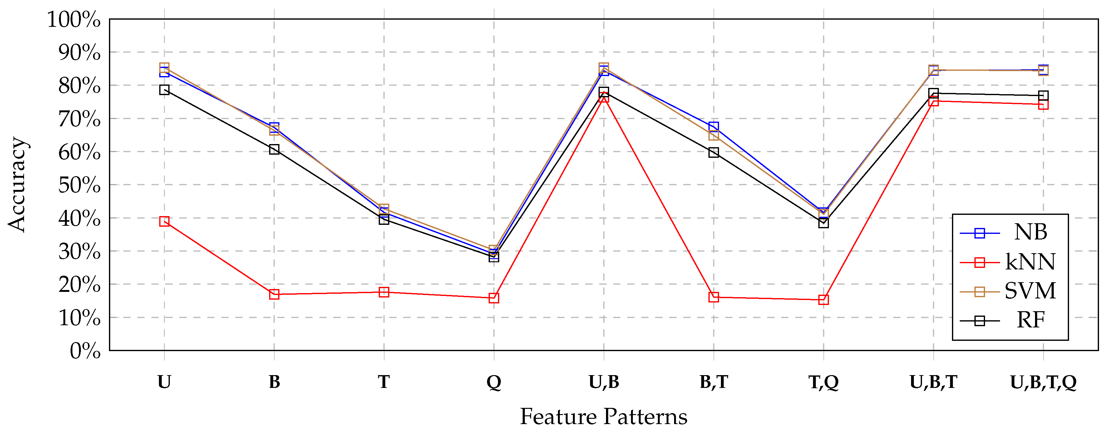
Figure 4 depicts the results obtained by each classifier for all feature patterns by using the full set of features extracted from the training set. The blue line depicts the results obtained by the Naïve Bayes classifier; the red line depicts the results obtained by the kNN classifier; the brown line depicts the results obtained by the SVM classifier, the black line depicts the results obtained by the Random-Forest classifier.

We can notice that the Naïve Bayes classifier (blue line) always performed as the best classifier, always obtaining the highest accuracy. The SVM classifier (brown line) performed only a little bit worse, but results were comparable. The Random Forest classifier still showed comparable accuracy, even though a little bit less than Naïve Bayes and SVM classifiers.

In contrast, the inability of the kNN classifier to exploit most of feature patterns was evident. In details, we noticed that for U, U,B, U,B,T and U,B,T,Q feature patterns, the kNN classifiers obtained results that were comparable with the other classifiers. Instead, for feature patterns that did not include uni-grams, the kNN classifier obtained very poor results.

Nevertheless, notice that the other three tested classification techniques suffered for the absence of uni-grams in the feature sets as well, even though they behaved better than the kNN classifier.

If we focus on results obtained by each classifier for feature patterns that contain uni-grams, it clearly appears that no advantage was obtained by combining uni-grams with other features. Looking at Table 4, we see that the Naïve Bayes classifier obtained a very slight improvement; in contrast, looking at Table 5, Table 6 and Table 7, we can see a slight deterioration of accuracy, when comparing the U pattern with U,B, U,B,T and U,B,T,Q combined patterns.

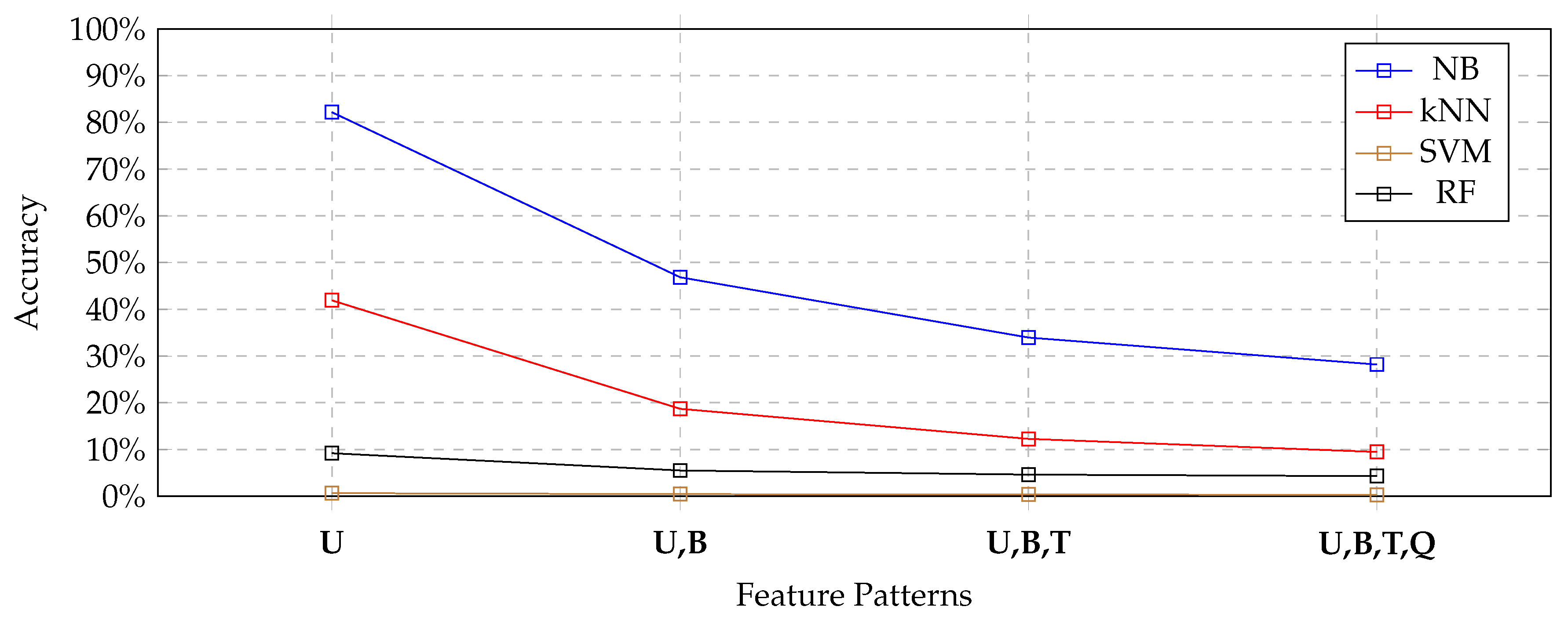
5.3. Sensitivity Analysis

We can now consider the sensitivity analysis we performed. Recall that, apart from the full set of features, we also considered the best 80%, 65% and 50% of features, on the basis of the weight defined in Formula 1.

Figure 5, Figure 6 and Figure 7 depict the results so far obtained, respectively, with the 80%, 65% and 50% of features. In the 80% case (Figure 5), no significant variations appeared: the performances obtained by all classifiers were, more or less the same. This is also confirmed by looking at the tables, that show very small reductions of accuracy. Nevertheless, the general behavior of the four classifiers remained exactly the same as for the full set of features. Consequently, we could argue that it was not the case to use the full set of features for training the classifiers, so as to save time and computational power.

Considering the 65% case (depicted in Figure 6), and the 50% case (depicted i Figure 7), we still observed a very slight reduction of accuracy. Only the kNN classifier behaved significantly worse with uni-gram patterns in the 50% case; nevertheless, looking at Figure 7, we notice that with patterns U,B,T and U,B,T,Q, the combined feature patterns that contained uni-grams helped the classifier to obtain good results.

In effect, looking at Table 5, we can see that both precision and recall strongly penalized the kNN classifier, with respect to the other competitors. This happened with all feature patterns.

5.4. Execution Times and Suitability Metric

Based on accuracy, the kNN classifier was not suitable for the investigated application context, while the other classifiers showed comparable performance. However, the cost of computation is an important issue, thus we also gathered execution times both for training and testing.

We performed experiments on a PC powered by Processor Intel(R) Core(TM) i7-5600U, with clock frequency of 2.60 GHz, equipped with 8 GB RAM; the operating system was Windows 10 Pro (64 bit).

Table 8. Execution times (in seconds) for the most promising feature patterns.

NB
Feature Pattern	Feature Extraction Time	Model Building Time	Total Training Time	Testing Time
U	0.0028	0.3626	0.3654	0.1572
U,B	0.0162	1.2932	1.3094	0.2905
U,B,T	0.0299	2.3124	2.3423	0.4124
U,B,T,Q	0.0434	3.2504	3.2938	0.4971
kNN
Feature Pattern	Feature Extraction Time	Model Building Time	Total Training Time	Testing Time
U	0.0028	0.3339	0.3367	5.1004
U,B	0.0162	1.2770	1.2932	5.0536
U,B,T	0.0299	2.2337	2.2636	5.7653
U,B,T,Q	0.0434	3.2577	3.3011	5.3663
SVM
Feature Pattern	Feature Extraction Time	Model Building Time	Total Training Time	Testing Time
U	0.0028	137.9433	137.9461	30.2422
U,B	0.0162	201.2421	201.2583	45.3217
U,B,T	0.0299	247.0215	247.0514	57.4804
U,B,T,Q	0.0434	281.5109	281.5543	62.1898
RF
Feature Pattern	Feature Extraction Time	Model Building Time	Total Training Time	Testing Time
U	0.0028	56.5771	56.5799	1.4356
U,B	0.0162	219.9926	220.0088	2.0941
U,B,T	0.0299	399.2106	399.2405	2.4720
U,B,T,Q	0.0434	617.9247	617.9681	2.6590

reports the execution times shown by the four classifiers on the full set of features, for the most promising feature patterns, i.e., U, U,B, U,B,T and U,B,T,Q. Specifically, we evaluated execution times during the training phase and during the test phase; notice that we also measured the execution times concerned with feature extraction, so as to understand how heavy the computation of Cartesian products of features was.

The first thing we can notice is that feature extraction was performed in a negligible time, if compared with the actual training performed by the classifier; even in the case of the most complicated feature pattern (i.e., U,B,T,Q), this time was negligible. Nonetheless, to obtain a given feature pattern, experiments confirmed that the library we adopted was deterministic, since the execution time was independent of the specific attempt.

In contrast, looking at the execution time for model building, the reader can see that there were significant differences. Consequently, in order to choose the best classifier, the cost of computation should be considered. For this reason, we defined a cost-benefit metric, in such a way accuracy represents the benefit, while execution time represents the cost. We called this metric Suitability, because by means of it we wanted to rank classifiers in order to find out the one that was suitable for our context.

Consider a pool of experiments $E=\{e_1,e_2,\cdots ,e_h\}$, where for an experiment $e_i$ we refer to its accuracy as $e_i.Accuracy$, to its training execution times as $e_i.trtime$ (the execution time shown during the training phase) and to the test execution times as $e_i.tetime$ (the execution time shown during the test phase). The Training Suitability of an experiment is defined as

$$TrainingSuitability\left(e_i\right)=e_i.Accuracy\times \frac{mintrtime}{mintrtime+(e_i.trtime-mintrtime)\times \beta }$$

(3)

where $mintrtime=mi{n}_{\forall e_i\in E}(e_i.trtime)$ (i.e., the minimum training execution time). $\beta$ is a importance weight of the difference between the training execution time of the $e_i$ experiment and the minimum training execution time; we decided to set it to $50\%$, in order to mitigate the effect of execution times on the final score; in fact, with $\beta =1$, the penalty effect would be excessive.

Similarly, we can define the Testing Suitability, defined in Formula 4.

$$TestingSuitability\left(e_i\right)=e_i.Accuracy\times \frac{mintetime}{mintetime+(e_i.tetime-mintetime)\times \gamma }$$

(4)

where $mintetime=mi{n}_{\forall e_i\in E}(e_i.tetime)$ (i.e., the minimum testing execution time among the experiments). Similarly to $\beta$, $\gamma$ is the relevance of the difference between execution time of the $e_i$ experiment and the minimum testing time. We decided to set it to $50\%$ as well.

Training Suitability and Testing Suitability ranked experiments by keeping the two phases (training and testing) separated.

In Formula 5, we propose a unified Suitability metric.

$$Suitability\left(e_i\right)=\alpha \times TrainingSuitability\left(e_i\right)+(1-\alpha )\times TestingSuitability\left(e_i\right)$$

(5)

i.e., the unified suitability is the weighted average of Training Suitability and Testing Suitability, where $\alpha \in [0,1]$ balances the two contributions.

Table 9. Suitability for the most promising feature patterns.

Feature Pattern	Classifier	TrainingSuitability	TestingSuitability	Suitability
U	NB	80.4512	83.8872	82.1692
U,B		34.4861	59.1987	46.8424
U,B,T		21.2401	46.6448	33.9425
U,B,T,Q		15.6920	40.6500	28.1710
U	kNN	79.0800	4.7289	41.9044
U,B		32.6185	4.7653	18.6910
U,B,T		20.3525	4.1720	12.2622
U,B,T,Q		14.4739	4.4506	9.4623
U	SVM	0.4153	0.8821	0.6487
U,B		0.2839	0.5875	0.4357
U,B,T		0.2287	0.4583	0.3435
U,B,T,Q		0.1994	0.4210	0.3102
U	RF	0.9263	15.4535	8.1899
U,B		0.2354	10.7576	5.4965
U,B,T		0.1283	9.1025	4.6154
U,B,T,Q		0.0828	8.4880	4.2854

reports the values of training suitability, testing suitability and unified suitability for the same experiments considered in Table 8. Figure 8 depicts the results, by using the same convention as in Figure 4, by using the unified suitability. The reader can see that the Naive Bayes classifier had the highest suitability values, due to its ability to combine high accuracy and very low execution times. Surprisingly, the kNN classifier obtained the second position; in fact, in spite of the fact that it obtained the worst accuracy values, it obtained the lowest execution times. Finally, the SVM classifier and the Random-Forest classifier were strongly penalized by their execution times.

Consequently, on the basis of Table 9 and Figure 8, we can clearly say that the Naive Bayes classifier applied to the feature pattern of uni-grams clearly emerged as the most suitable solution for our application context (presented in Section 3) and specifically to solve Problem 1.

6. Conclusions and Future Work

In this paper, we have posed the basic brick towards the extension of micro-blog user interfaces with a new functionality: a tool to recommend users with other users to follow (influencers) on the basis of topics their message talk about. The basic brick is a text classification technique applied to a given feature pattern that provides good accuracy by requiring limited execution times. To identify it, we built an investigation framework, that allowed us to perform experiments, by measuring effectiveness (accuracy) and execution times. A cost-benefit function, called Suitability, has been defined: by means of it, we discovered that the best solution to address the problem is to apply a Naive Bayes classifier to uni-grams extracted from within messages, both to train the model and to classify unlabeled messages. We considered execution times because, in our opinion, the envisioned application scenario asks for fast functionalities; thus execution times emerge as critical factors. At the best of our knowledge, this comparative study of performances shown by classifiers, based on both accuracy and execution times, is a unique contribution of this paper.

The next steps towards the more ambitions goal of building a recommender system for influencers is to develop the surrounding methodology that actually enables to recommend influencers: in fact, once messages are labeled with topics, it is necessary to rank potential influencers, on the basis of the frequency with which they post messages about a given topic. This methodology will be the next step of our work.