Remote Sensing Scene Classification and Explanation Using RSSCNet and LIME

Abstract

Classification is needed in disaster investigation, traffic control, and land-use resource management. How to quickly and accurately classify such remote sensing imagery has become a popular research topic. However, the application of large, deep neural network models for the training of classifiers in the hope of obtaining good classification results is often very time-consuming. In this study, a new CNN (convolutional neutral networks) architecture, i.e., RSSCNet (remote sensing scene classification network), with high generalization capability was designed. Moreover, a two-stage cyclical learning rate policy and the no-freezing transfer learning method were developed to speed up model training and enhance accuracy. In addition, the manifold learning t-SNE (t-distributed stochastic neighbor embedding) algorithm was used to verify the effectiveness of the proposed model, and the LIME (local interpretable model, agnostic explanation) algorithm was applied to improve the results in cases where the model made wrong predictions. Comparing the results of three publicly available datasets in this study with those obtained in previous studies, the experimental results show that the model and method proposed in this paper can achieve better scene classification more quickly and more efficiently.

1. Introduction

With the gradual advancement of technology today, smart mobile devices and aerial cameras are beginning to appear on the market. As the performance of the hardware improves, aerial photography technology is constantly improving along with it, and rapid breakthroughs in imaging technology have made it possible to acquire imagery quickly. There are more types of imagery than ever before and the imagery is also clearer than was possible previously. Remote sensing images can be used in many technical aspects of scene classification, such as land-cover detection, urban planning, disaster relief, traffic control, etc. Therefore, how to classify large amounts of remote sensing image data covering land areas is an important research topic [1,2,3,4,5,6,7,8].

In the past, when using image data for classification research, the primary focus was on how to effectively perform the task of feature extraction [9,10]. The deep-learning methods used today make use of different convolutional neural network models to automatically perform feature recognition, extract the required image details, and then train the classification model to recognize the scene. The popularization of graphics cards in recent years has enabled the amount of time spent on deep learning in neural network model training to be reduced. It has also enabled the rapid development of deep-learning research and studies related to the classification of high-resolution remote sensing images [11,12,13].

Related parameters used in deep-learning models include the training methods, network architecture, optimizer design, hardware operation, etc. Adjusting the model training hyper-parameters is a very important aspect of the model design. Smith [14] proposed a new learning-rate method; instead of a fixed value, a cyclical learning policy was set for the model being trained. The results showed that this could effectively reduce the number of training iterations and improve the accuracy of the classification. Smith and Topin [15] then proposed a new super-convergence one-cycle cyclical learning policy and suggested the usage of a large learning rate for model training, which, according to them, can improve the model’s generalization capability. More recently, Leclerc and Madry [16] explored the impact of different learning rates on deep learning and found that the low and high values of cyclical learning rates [14,15] concur with their two regimes.

Training is the process of learning and adjusting the parameters of a model. During training, iteration methods such as the gradient descent learning algorithm are commonly used. Early stopping [17] is a method often used during training to prevent overfitting. This method calculates the accuracy of the test dataset during model training. When the accuracy of the test data no longer improves, the training stops and is terminated early. This not only helps to prevent overfitting of the training model but also improves the model’s generalization ability.

This study aimed to produce an improved model with enhanced detection ability and a small number of training iterations. A two-stage circular learning method for training was, therefore, proposed. First of all, the image features were obtained by transfer learning; the classification framework designed in this paper was then used for training. The two-stage circular learning rate was used to reduce the number of iterations and, finally, the best model weights were obtained using the early stopping method. The main contributions of this paper are as follows:

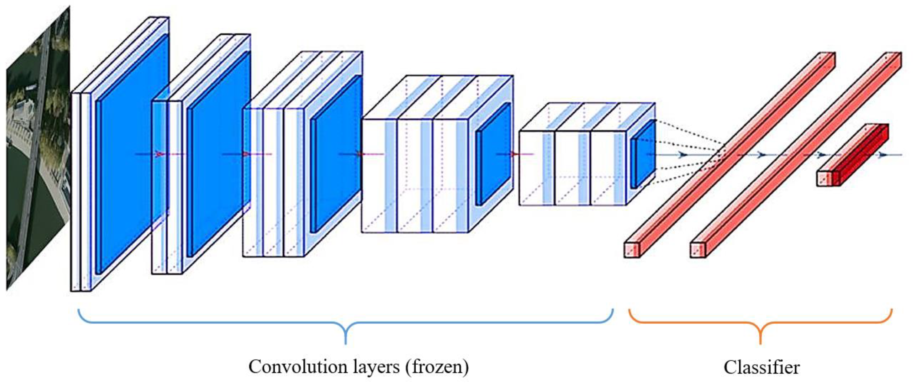
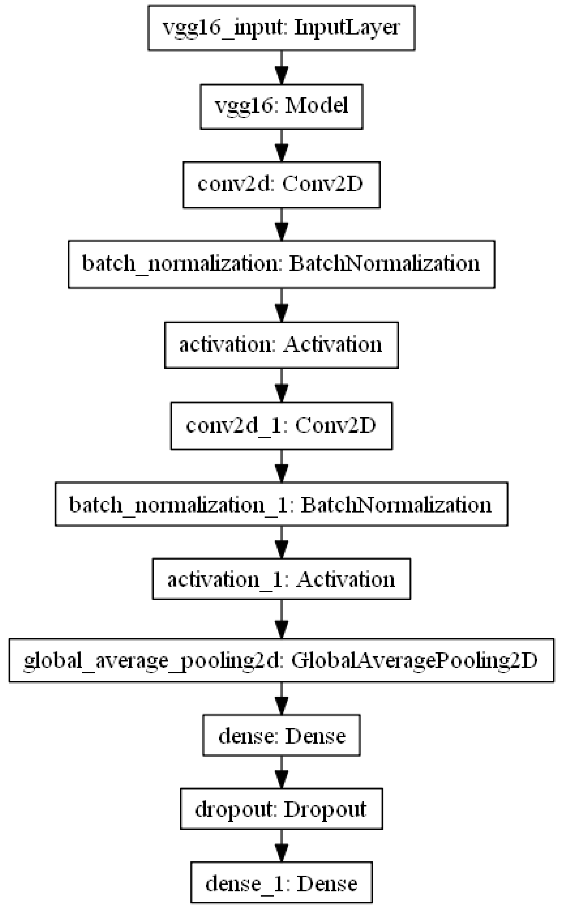
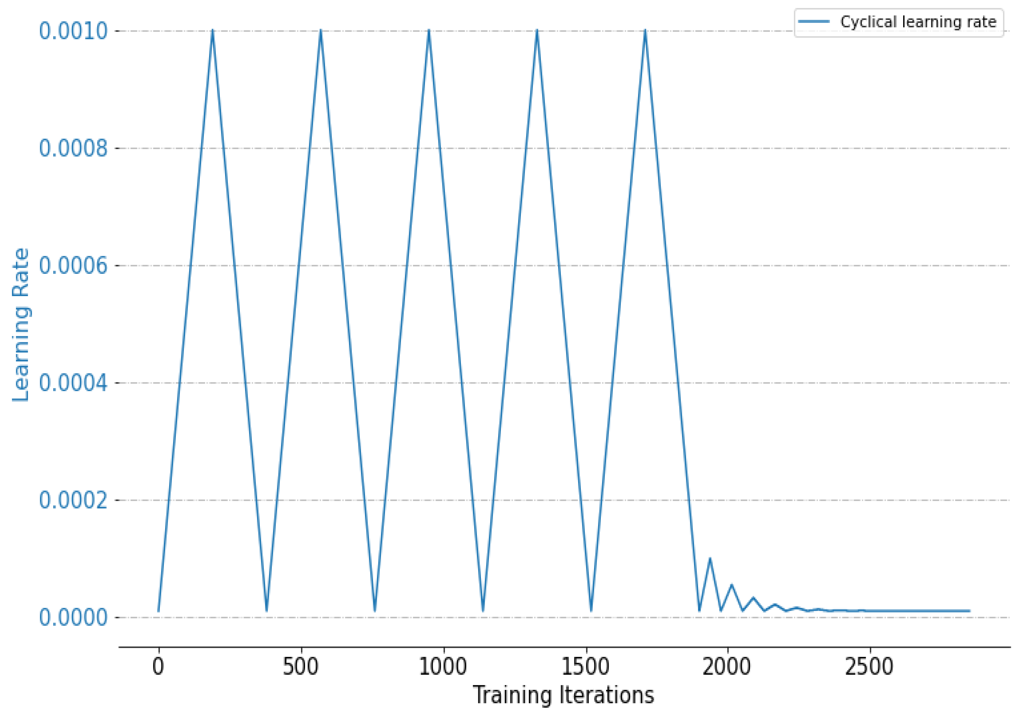
• In order to reduce model overfitting and to obtain models with a high generalization capability, we recommend a new CNN (convolutional neutral networks) architecture, i.e., RSSCNet (remote sensing scene classification network), integrated with the simultaneous use of a two-stage cyclical learning-rate training policy and the no-freezing transfer learning technology that requires only a small number of iterations. In this way, an excellent level of accuracy can be obtained.
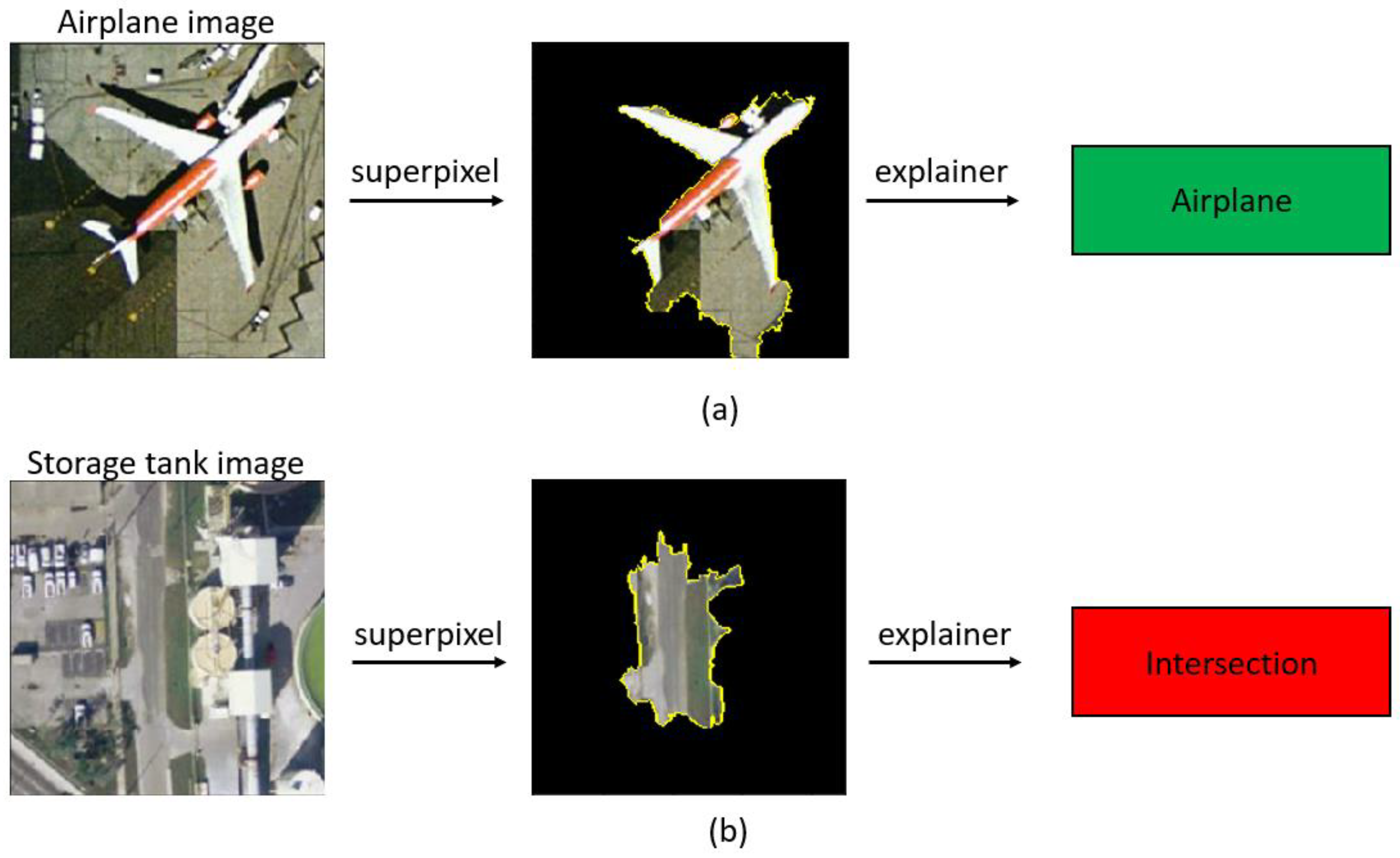
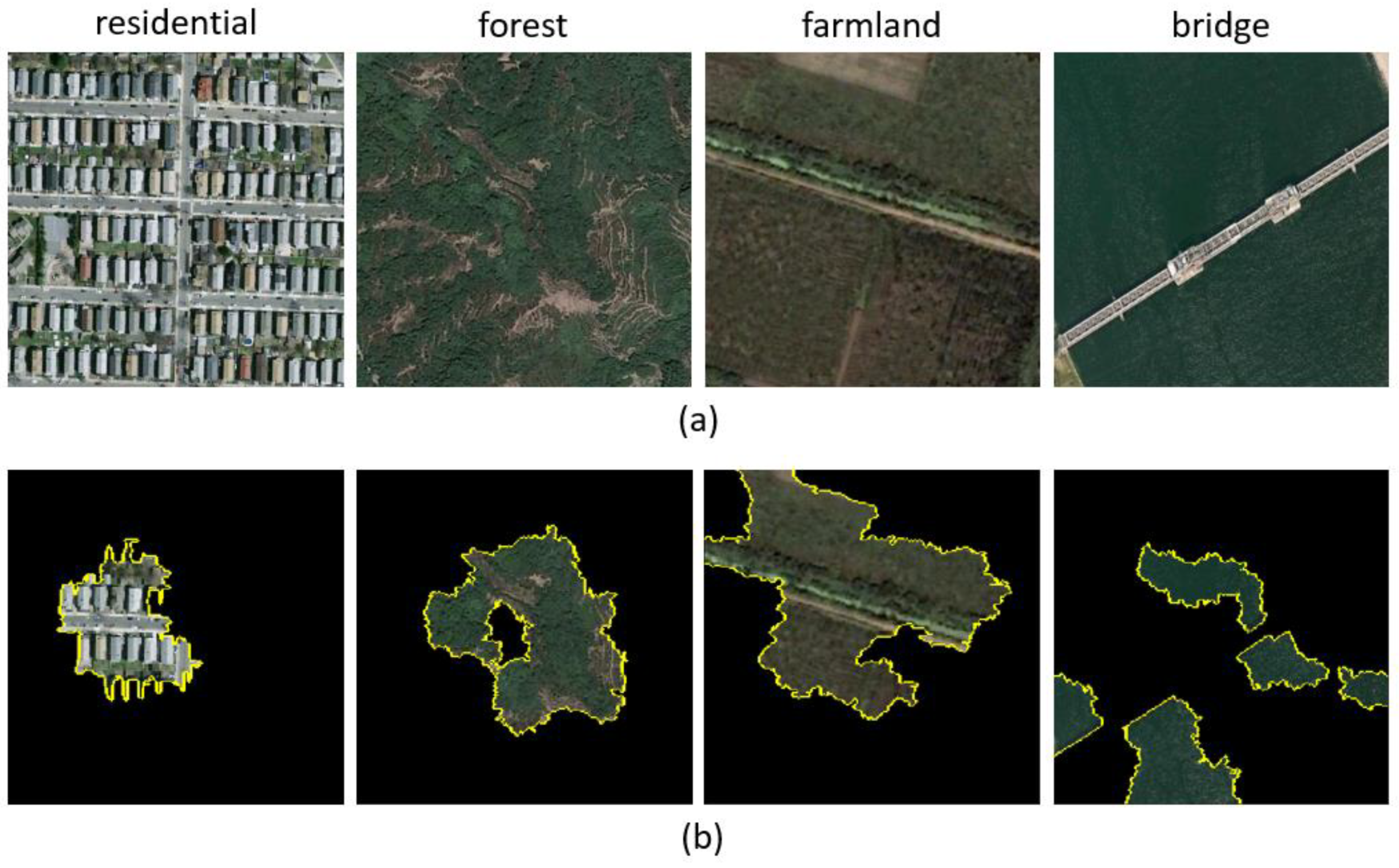
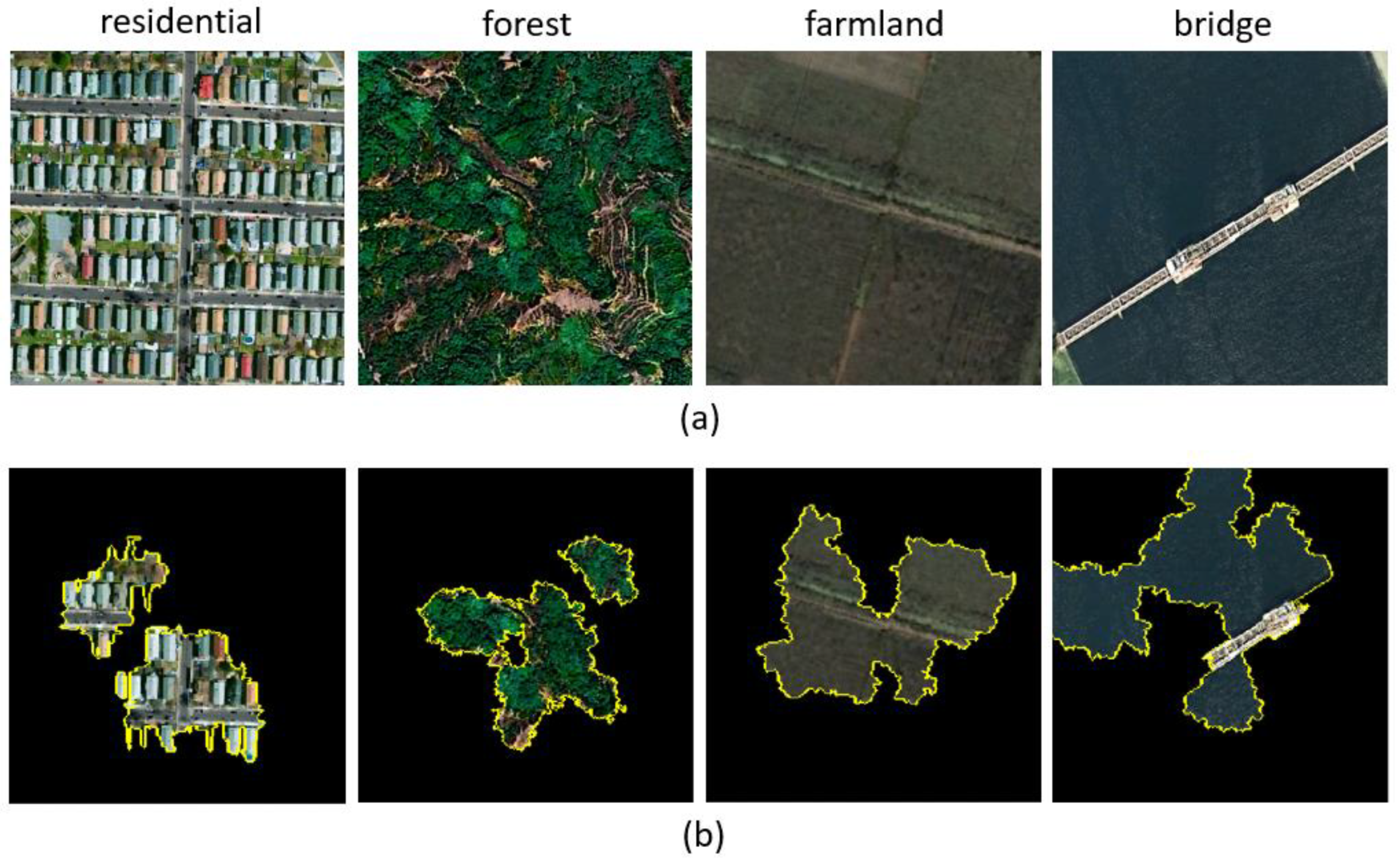
• By using the LIME (local interpretable model, agnostic explanation) super-pixel explanation, the root causes of model classification errors were made clearer and a further understanding was obtained. After the image correction preprocessing on the misclassified cases in the WHU-RS19 [18] dataset, this correction procedure was found to improve the overall classification accuracy. We hope that readers can better understand the reasoning mechanism of AI models for remote sensing scene classification.

The remainder of this paper is organized as follows: the dataset is introduced in the second section. In the third section, the steps of the developed research method are explained in detail. The data results and results from other studies are discussed in the fourth section, along with an analysis of why improved results were obtained using the proposed method. The fifth section is the conclusion.

2. Datasets

In this study, three publicly available remote sensing image data sets—the UC Merced land-use dataset [19], RSSCN7 [20], and WHU-RS19 [18]—were used for testing the performance of the proposed method.

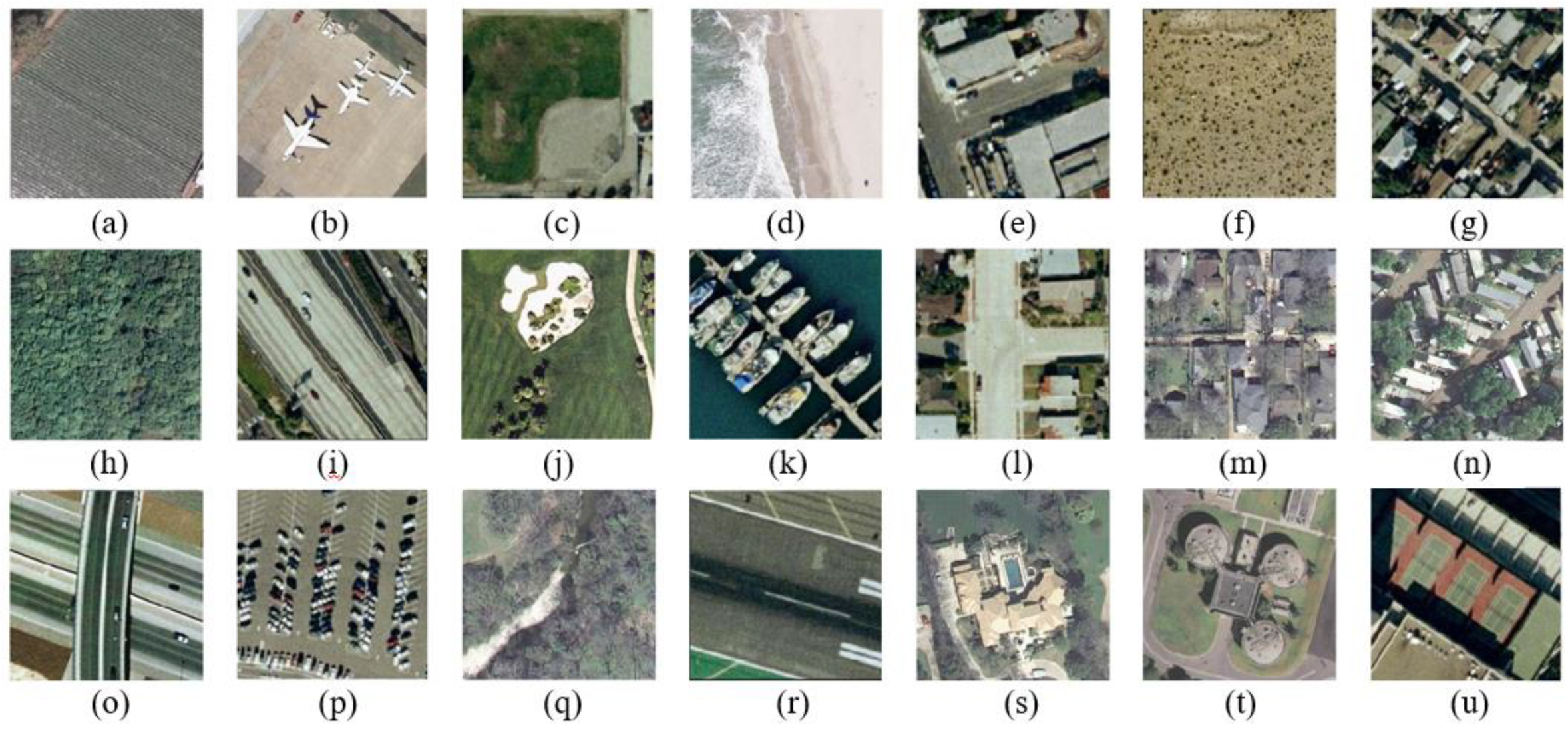
2.1. UC Merced Land-Use Dataset

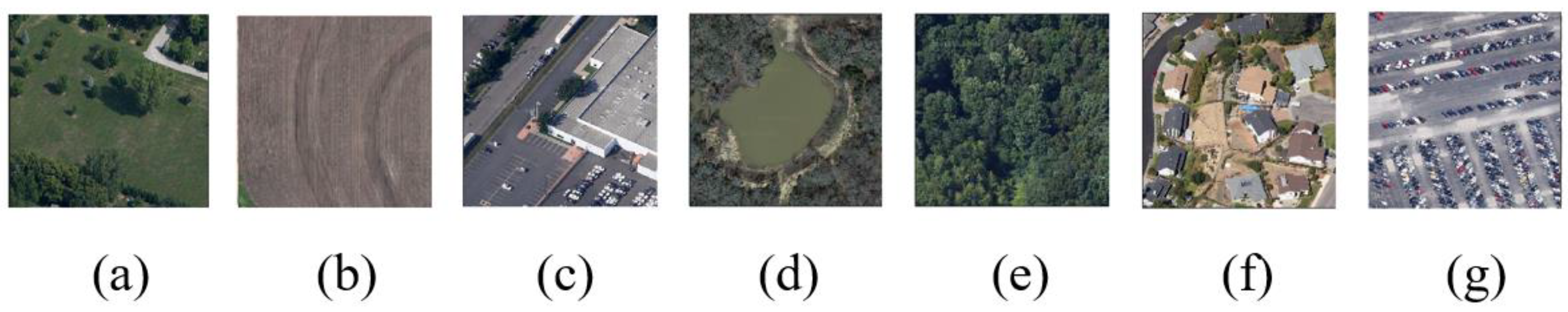
The pixel resolution of the UC Merced land-use dataset is 1 ft (=0.3048 m), and the dataset contains a total of 2100 images. The images are composed of 21 different land-use types; each class of each image has 100 RGB color images. The land-use types include agricultural, airplane, baseball diamond, beach, buildings, chaparral, dense residential, forest, freeway, golf course, harbor, intersection, medium residential, mobile home park, overpass, parking lot, river, runway, sparse residential, storage tanks, and tennis court. All the images contain different textures and colors, as shown in Figure 1. The UC Merced land-use dataset images were converted into 224 × 224 pixel size for transfer learning.

2.2. RSSCN7 Dataset

The RSSCN7 dataset is a public dataset released by Wuhan University in 2015. There are seven different scene categories, including grass, field, industry, river, lake, forest, residential, and parking lot. The entire dataset includes a total of 2800 images. Each scene category of the dataset contains 400 images and corresponds to one of four different sampling ratios (1:700, 1:1300, 1:2600, and 1:5200); there are 100 images corresponding to each of these ratios. In the original dataset, all of the images have a size of 400 × 400 pixels. The data were acquired in different seasons and under various weather conditions. In the case of sampling differences in different proportions, classification of this dataset is a greater challenge. The different image categories are shown in Figure 2. The RSSCN7 dataset images were converted into 224 × 224 pixel size for transfer learning.

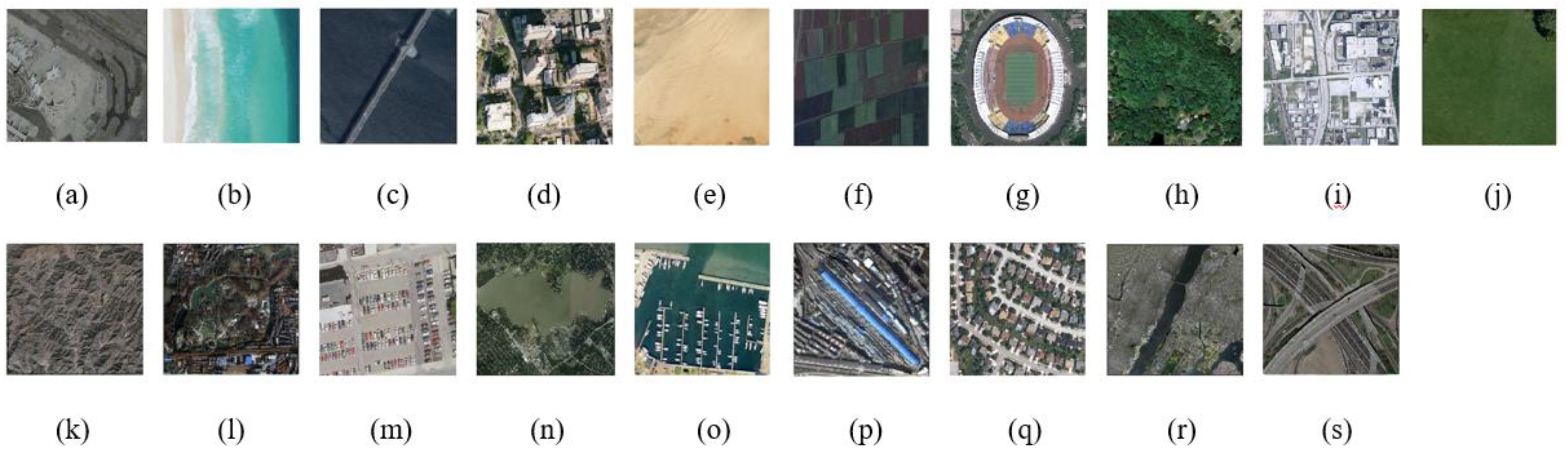
2.3. WHU-RS19 Dataset

The WHU-RS19 dataset was extracted from Google Earth satellite imagery. The spatial resolution of these satellite images is up to 0.5 m, and the spectral bands are red, green, and blue. There are 19 scene categories, including airport, beach, bridge, commercial, desert, farmland, football field, forest, industrial, meadow, mountain, park, parking, pond, port, railway station, residential, river, and viaduct. There are about 50 images corresponding to each category, and the entire dataset contains a total of 1005 images. The original image size is 600 × 600 pixels. Because the resolution, scale, direction, and brightness of the imagery vary greatly, processing this dataset is somewhat challenging. These data are also widely used in evaluating various scene classification methods. Figure 3 shows some samples from the dataset. The WHU-RS19 dataset images were converted into 224 × 224 pixel size for transfer learning.

3. Method

In this section, the model training method used in the experiments is introduced along with the convolutional neural network model used in this study and the two-stage cyclical learning-rate numerical design method used for the training.

3.1. Convolutional Neural Network Model

To start, the VGG [21] neural network trained by ImageNet was used as the model for image feature extraction. This method adjusts the structure of the neural network used for certain trained network models by using transfer learning to perform other image training tasks. In the experiments carried out in this study, the structure of the original neural network layer was adjusted by freezing the weights in one or more layers of the original model, minus the time to retrain the deep model. The original model was used for feature extraction, and the newly embedded model layer was trained for use in classification. It was, therefore, only necessary to update and modify the weights of the newly added network layer during training; the frozen layer weights that were transferred from the learning model could be kept, as shown in Figure 4 [22].

After removing the top-level fully connected layers of the pre-training model, a new classification network was added. In our model, we chose an exponential linear unit (ELU) [23] as our activation function because it can reduce the vanishing gradient problem by identifying positive values. The ELU has negative values; hence, it allows the mean unit to approach zero for a deep neural network model and obtain a faster convergence than the rectified linear unit (ReLU). Regularization was also added as a tool to reduce overfitting in the network. Regularization can be considered as a penalty term in the loss function. The so-called “penalty” refers to restrictions that are applied to some parameters in the loss function to prevent overfitting. Moreover, we added a batch normalization layer [24] after the convolution layer in our model, which can act as a regularizer to decrease overfitting. Batch normalization can use a larger learning rate in model training to achieve faster convergence benefits.

Considering the balance between the network capacity and the test accuracy and discussing the influence of different regularization and optimization strategies, we finally designed this new deep learning network architecture with a high generalization capability. The proposed CNN architecture is called RSSCNet (Figure 5). In RSSCNet, the depth of the weight layers is 17, and the mathematical formulation is written as follows:

$$\left\{\begin{array}{c}X=f^{\left(16\right)}\left(f^{\left(15\right)}\left(\cdots \left(f^{\left(2\right)}\left(f^{\left(1\right)}\left(\mathit{x},\mathit{w},\mathit{b}\right)\right)\right)\right)\right)\\ Y=Softmax\left(X\right)\end{array}\right\},$$

(1)

where $\mathit{x}$ is the input data of each image, $\mathit{w}$ is the weight matrix, $\mathit{b}$ is the bias, $X$ is the representative feature of $\mathit{x}$, and $Y$ is the output probability. The RSSCNet architecture includes 15 convolutional layers, five max pooling layers, one global average pooling layer, two batch normalization layers [24], one dropout layer, and two fully connected layers with a softmax classification. Note that the activation function of the last two convolutional layers uses an ELU [23], while the other weight layers use the ReLU activation function. The convolution filter size is 3 × 3. The dropout rate is 0.5. The regulations of L1 and L2 are 0.01 and 0.02, respectively.

3.2. Image Data Augmentation

When training deep-learning models, large amounts of data are needed for training, and it is necessary to try to avoid overfitting during the training. Proper use of regularization strategies related to deep learning, such as L1/L2 regularization, dropout, batch normalization, early stopping, and data augmentation, is needed. Among these strategies, data augmentation is regarded as an effective method for training a generally applicable model using limited training data [25]. In data augmentation, after the image is rotated, resized, scaled, and flipped, or has its brightness or color temperature changed, the original image in the dataset is changed to create more images that will allow the model to continue learning. In order to make up for the lack of data, in this study, an augmented training method was included in the training. After using horizontal and vertical flipping processing, the training image was increased by small-scale translation and scaling in order to enhance the generalization ability of the model.

3.3. Cyclical Learning Rate

The learning-rate method proposed by Smith [9] sets cyclical learning rates for the model instead of a fixed value and uses this to train the model. Results show that this can improve the accuracy of the classification and reduce the need for trivial adjustments. During training, the number of iterations used is usually reduced, and there are three different cyclical ways in which the learning-rate loop method can learn: “triangular”, “triangular2”, and “exp_range”. In our research, a two-stage cyclical learning-rate method was used to train the model. In the first stage, the “triangular” method was used to quickly find the best solution in the model; using this method, it was possible to avoid falling into a local solution when the learning rate was large. At the second stage, using the traingular2 method, the learning-rate cycle was gradually reduced to confine the model results until, finally, the solution stayed at a fixed position with no large swings (see Figure 6).

The proposed two-stage cyclical learning rate method is calculated as shown in Equation (2).

$$\left\{\begin{array}{c}z=\left|1+\frac{i}{\Delta }-2\ast \left[1+\frac{i}{2\Delta }\right]\right|\\ D=\left\{\begin{array}{c}1,forstage1\\ {\left(\frac{l{r}_{min}}{l{r}_{max}}\right)}^{\left(\frac{\left[\frac{i}{2\Delta }\right]}{\left[\frac{i_{max}}{2\Delta }\right]}\right)},forstage2\end{array}\right\}\\ lr=l{r}_{min}+\left(D\ast l{r}_{max}-l{r}_{min}\right)\ast max\left(0,\left(1-z\right)\right)\end{array}\right\},$$

(2)

where $z$ is a dummy variable, $i_{max}$ is the total number of training epochs $i$, $\Delta$ is the step size that is equal to the half cycle length, $D$ is the damping factor, $lr$ is the cyclical learning rate, $l{r}_{min}$ is the minimum learning rate, and $l{r}_{max}$ is the maximum learning rate.

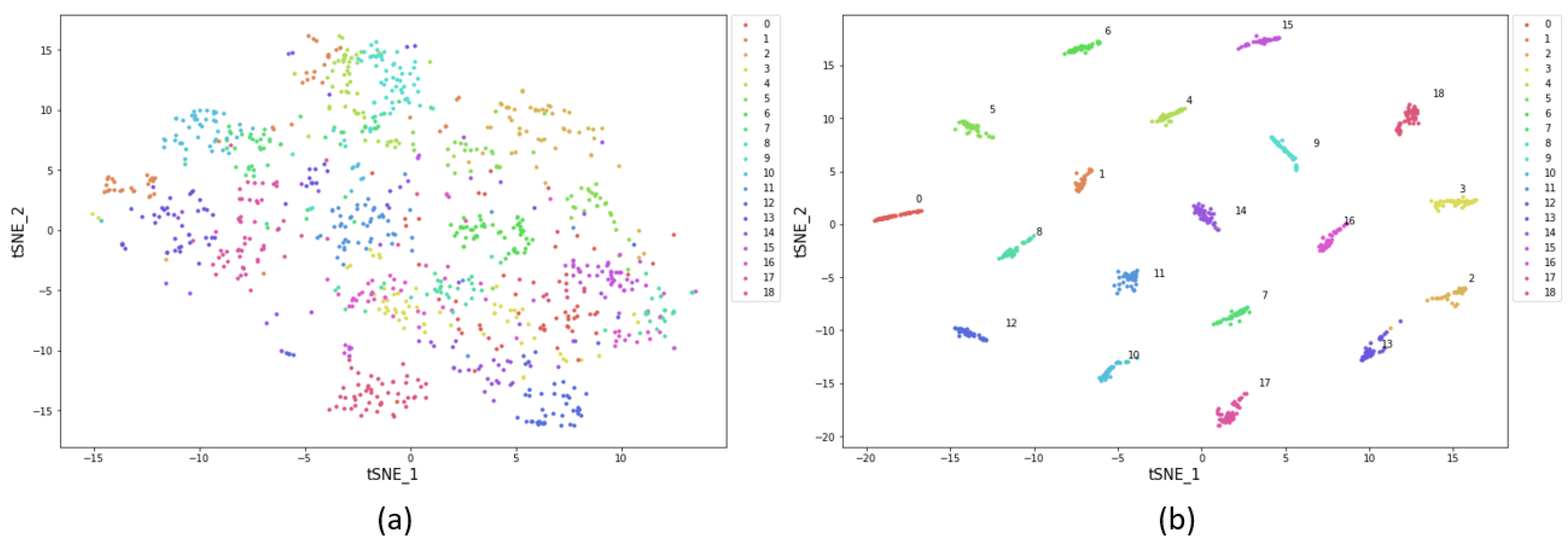
3.4. t-Distributed Stochastic Neighbor Embedding (t-SNE) Analysis Method

The t-SNE analysis method is a nonlinear dimensionality reduction algorithm used for exploring high-dimensional data. Laurens van der Maaten and Geoffrey Hinton [26] proposed a new technique for visualizing similarity data in 2008. This technique can not only retain the partial structure of the data but can also display clusters of multiple scales at the same time. The t-SNE algorithm can project data into two-dimensional or three-dimensional space and uses good visualization to verify the effectiveness of the dataset or algorithm. The t-SNE method was used in various fields as a visualization method to evaluate the quality of classification [27,28]. It uses conditional probability and a Gaussian distribution to define the similarity between sample points in high and low dimensions and uses KL (Kullback–Leibler) divergence to measure the similarity between the sum of two conditional probability distributions; it also uses it a value function to decrease complexity by using the gradient method. The t-distribution is used to define the probability distribution at low dimensions to alleviate the congestion caused by dimensional disasters.

3.5. LIME Model Explanation Kit

Although a deep learning model can obtain quite good classification results, it is difficult to understand how the classification results are derived because of its black-box characteristics. How to interpret the reasoning mechanism of the deep-learning model has become an important topic of research. In recent years, among the deep-learning methods, LIME is a new evaluation method for the interpretability of the model [29], i.e., whether it is possible to understand the importance of the deep-learning model for the interpretability of the image in the subsequent classification and prediction. The problem with model interpretability is that it is difficult to define the decision boundary of the model in a way that humans can understand. As shown in Figure 7, LIME is a Python library that attempts to generate some local feature-circle super-pixels. This can be used to explain the principle on which the model is based, which is usually difficult to describe, and to help with understanding whether the basis on which the model applies its decisions is appropriate or not. Figure 7a shows that the most interesting super-pixel of the RSSCNet model contains an airplane; hence, it can be correctly classified by the RSSCNet model. Figure 7b depicts that there is no storage tank in the super-pixel unlike the RSSCNet model, thereby causing the RSSCNet model to make a misclassification.

4. Results and Analysis

4.1. Experimental Set-Ups

4.1.1. Implementation Details

In this study, the tensorflow2.0 suite within Python was used as the platform for the experiment. The hardware and system configuration included a Windows 10 version 1703 system. An NVIDIA GTX 1080 TI graphics card was used; the computing core was an i7-6700 3.40 GHz 8-core central processing unit (CPU) with 32 GB memory. Different pre-trained model parameter settings were used, and the results of using these were compared. Attempts were made to adjust the settings for training methods with different stages. The size of the batches in the experiment was set to a uniform size of 64, which was more in line with the memory capacity of the graphics card; the image length and width were set to 224 pixels in all cases. This study designed the training set size based on earlier studies. For the UC Merced land-use dataset, two training configurations—80% training and 50% training—were used. For the RSSCN7 dataset, 50% training and 20% training were used, and, for the WHU-RS19 dataset, the two modes used were 60% training and 40% training Two modes and 10 repeated random training cycles were used to verify and evaluate the experimental results.

4.1.2. Evaluation Methods

In this experiment, the confusion matrix and the overall accuracy were used to evaluate the classification performance, and the results were compared with those obtained using other, recently developed methods. The confusion matrix can be applied to the performance analysis of two-class or multi-class classification. After the model made its predictions, each class was assigned to one of a group of tables so that the data could be displayed and so that the detailed classification results for each category after the predictions were made could be seen. To evaluate the accuracy of the classification results, the overall accuracy was used. The accuracy ranged from 0 to 1, where a closer number to 1 denotes better classification performance. The total number of images that were correctly classified was divided by the number of test images.

In addition to the confusion matrix, the kappa coefficient is also often used to analyze the difference in the classification results for indicators of the multi-category classification quality. This coefficient is a method used in statistics to evaluate consistency. It calculates the index of the overall consistency and the classification consistency. The value range is [−1, 1]. A higher coefficient value denotes higher accuracy of the classification achieved by the model. The kappa coefficient ($K$) calculation formula with a higher degree is expressed as follows:

$$K=\frac{\left(P_0-P_c\right)}{\left(1-P_c\right)}.$$

(3)

4.2. Results and Analysis

4.2.1. Analysis of Experimental Parameters

In this study, different pre-trained models were tested for the evaluation of the classification results. This was done so that the best feature extraction method for the appropriate pre-trained model could be found. Once it was found, the weight layers in the pre-trained model were adjusted. It was considered whether the pre-trained model weights would affect the results of the transfer learning in order to find the best training-layer training plan for the model parameter configuration that would be used in subsequent experiments in this study.

1.

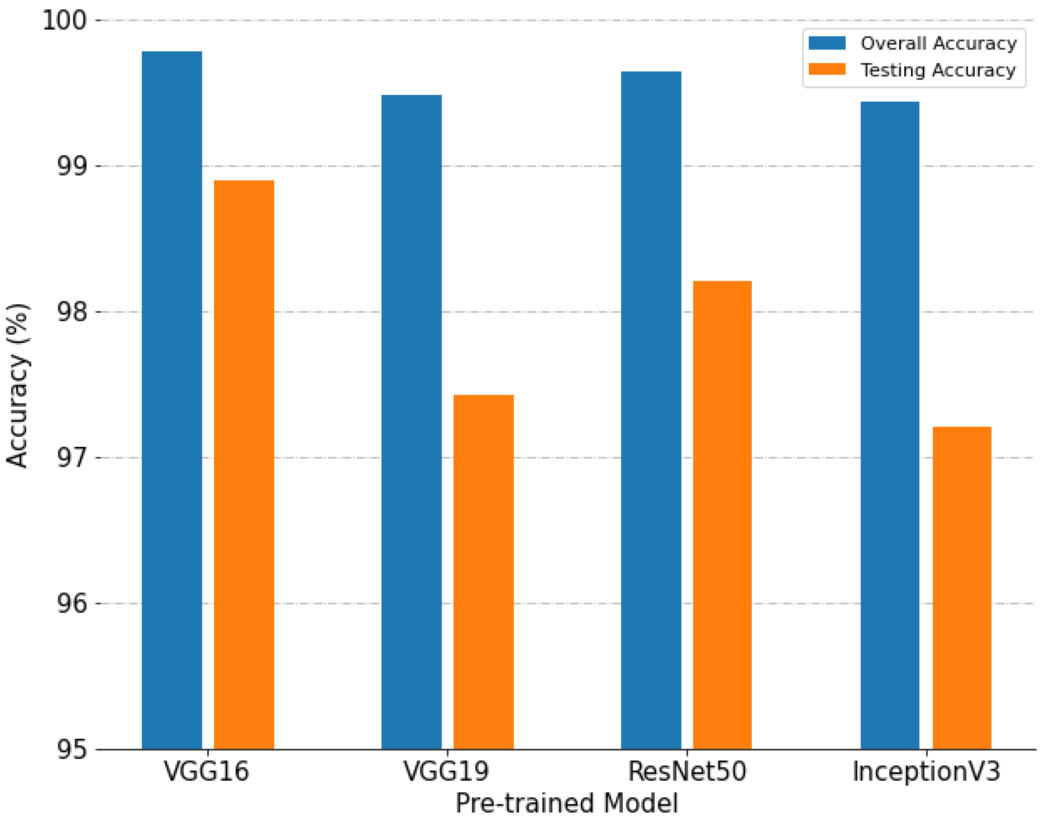
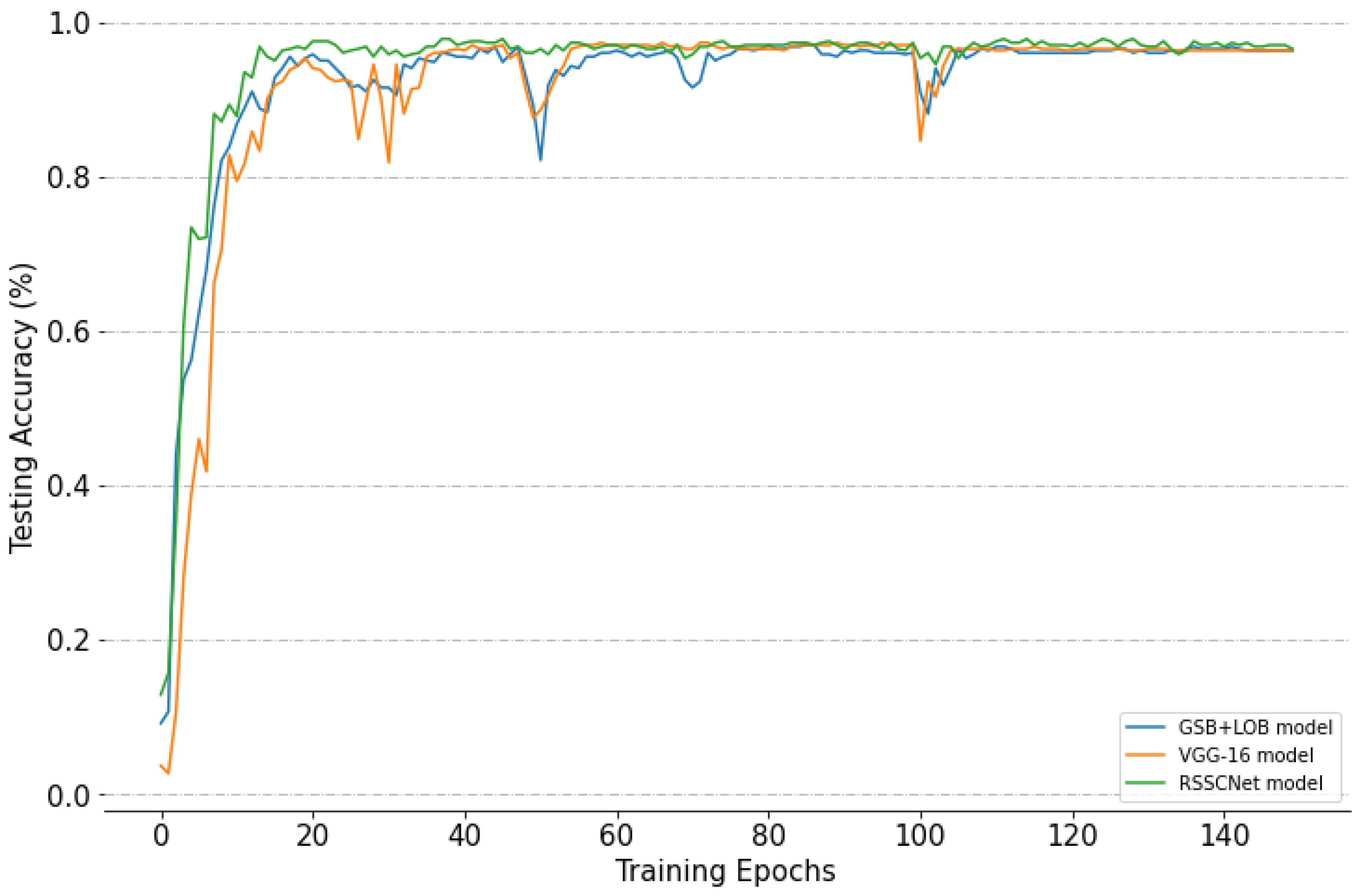
Different pre-trained CNN models

Different pre-trained models have different degrees of influence on image feature extraction. In this experiment, the WHU-RS19 dataset was used to embed four different common pre-trained models—VGG16 [21], VGG19 [21], ResNet50 [30], and InceptionV3 [31]—into the classification model. A classification performance test was carried out to help decide which of the four models was the most suitable for use as the pre-trained model. The training used an Adam optimizer; the batch size was 64, and the number of iterations was 150. The results of the training carried out using the four different models are shown for comparison in Figure 8. The results show that the pre-trained VGG16 model had the best overall accuracy; thus, in subsequent testing, this was used as the image feature extraction model.

2.

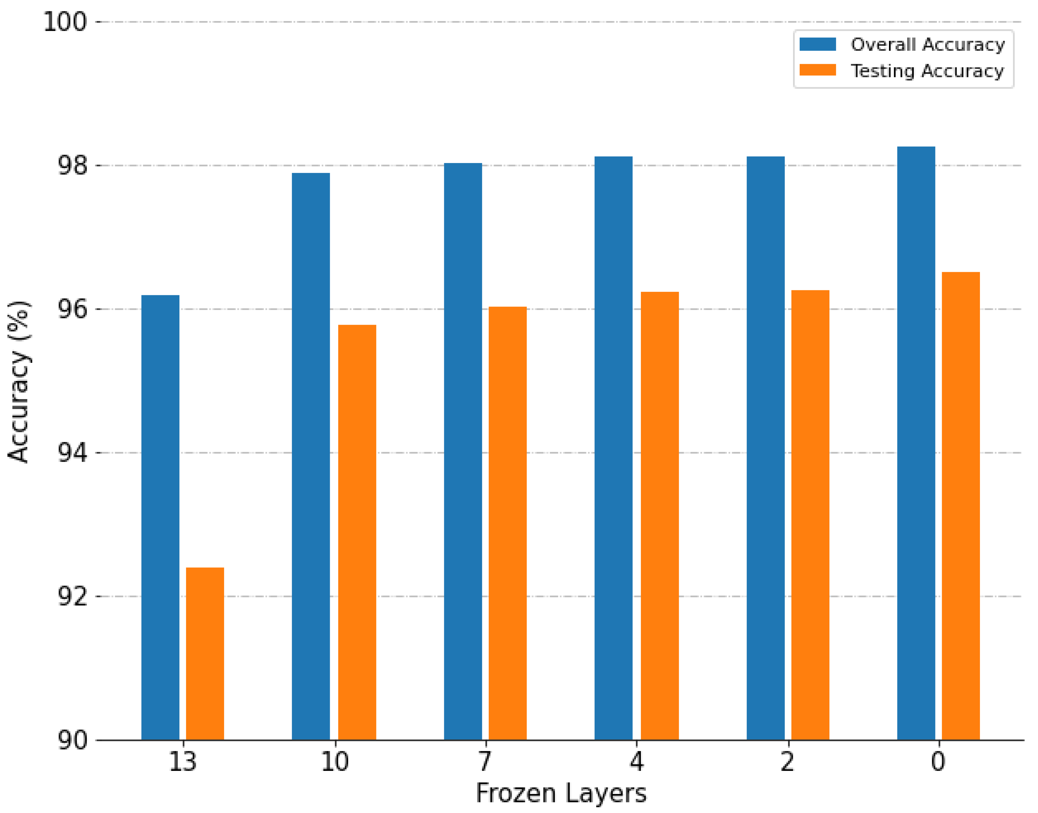
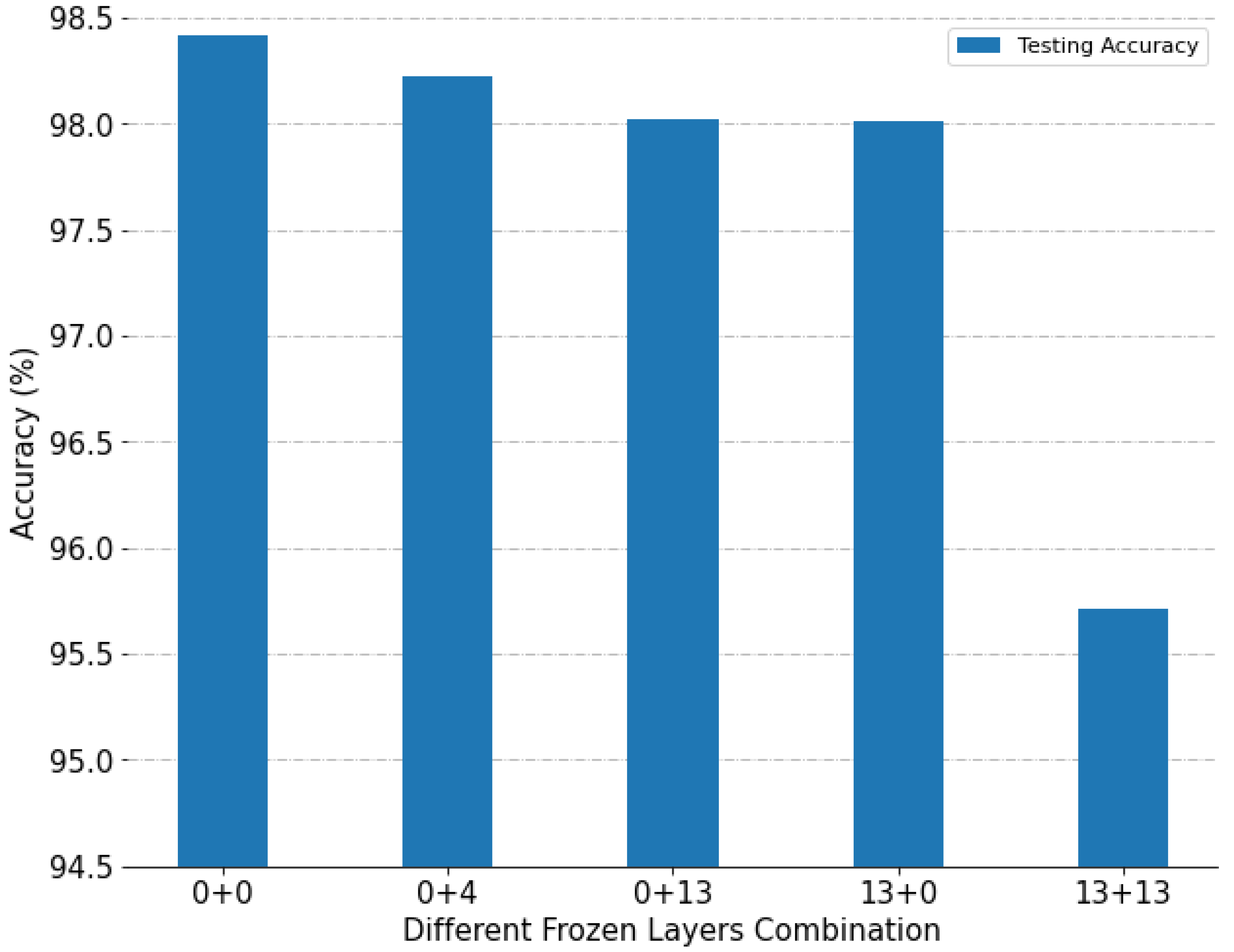
Different numbers of fine-tuning layers during training

After choosing to use the VGG16 pre-trained model, this study further explored whether, by freezing some of the network layers in the pre-trained model, the model could be made to have a better generalization performance. This experiment was also conducted using the WHU-RS19 dataset, and the results are shown in Figure 9. Based on the four blocks contained in the VGG16 model, two, four, seven, 10, and 13 layers were frozen. The results show that, when no layers were frozen, all the layers of the pre-trained model were retrained and fine-tuned, which means that, although this method requires more resources and a longer training time, it can produce a better overall accuracy. This shows that, in the classification of remote sensing images, the feature image that is required can be obtained by further training.

For the different fine-tuning layers discussed, the main consideration was whether to retrain the weights in the pre-trained model. Retraining the entire network inevitably takes a lot of time. However, in the process of feature extraction, in addition to training, we believe that it is necessary to focus on the training of the classifier and, hence, in this study, we aimed to strengthen the model’s ability to classify features by using a two-stage training method. In Figure 10, the WHU-RS19 dataset is used as the comparison dataset for the proposed method.

A two-stage training method (shown as “2-stage” in Figure 10) in our research indicates that two different optimizers were used and separated into two parts for the two-stage training. In the first stage, the SGD (stochastic gradient decent) optimizer was used to carry out 100 training iterations to train the entire neural network model. In this stage, the pre-trained model and classifier model could be adjusted at the same time, thus strengthening the features of the capture model and learning the classification ability. In the second stage of the training, the model weights with the best accuracy learned in the first stage were loaded, and the Adam optimizer was used to carry out the next 50 training iterations. We also compared the result with only using the Adam optimizer training for 150 iterations (shown as “1-stage” in Figure 10). As can be seen from Figure 10, the test accuracy obtained using the two-stage training (97.76%) was better than that obtained using the one-stage training (96.33%).

3.

Different classification architectures

For a performance comparison, we compare the RSSCNet architecture proposed herein with the other architectures in the literature, such as VGG-16-Net [21] and the GSB + LOB model [32]. Figure 11 showed the ranking results of the test accuracy of each model (i.e., RSSCNet: 0.978, VGG-16-Net: 0.973, and GSB + LOB model: 0.97), which indicated that the proposed RSSCNet is the best classification model.

4.

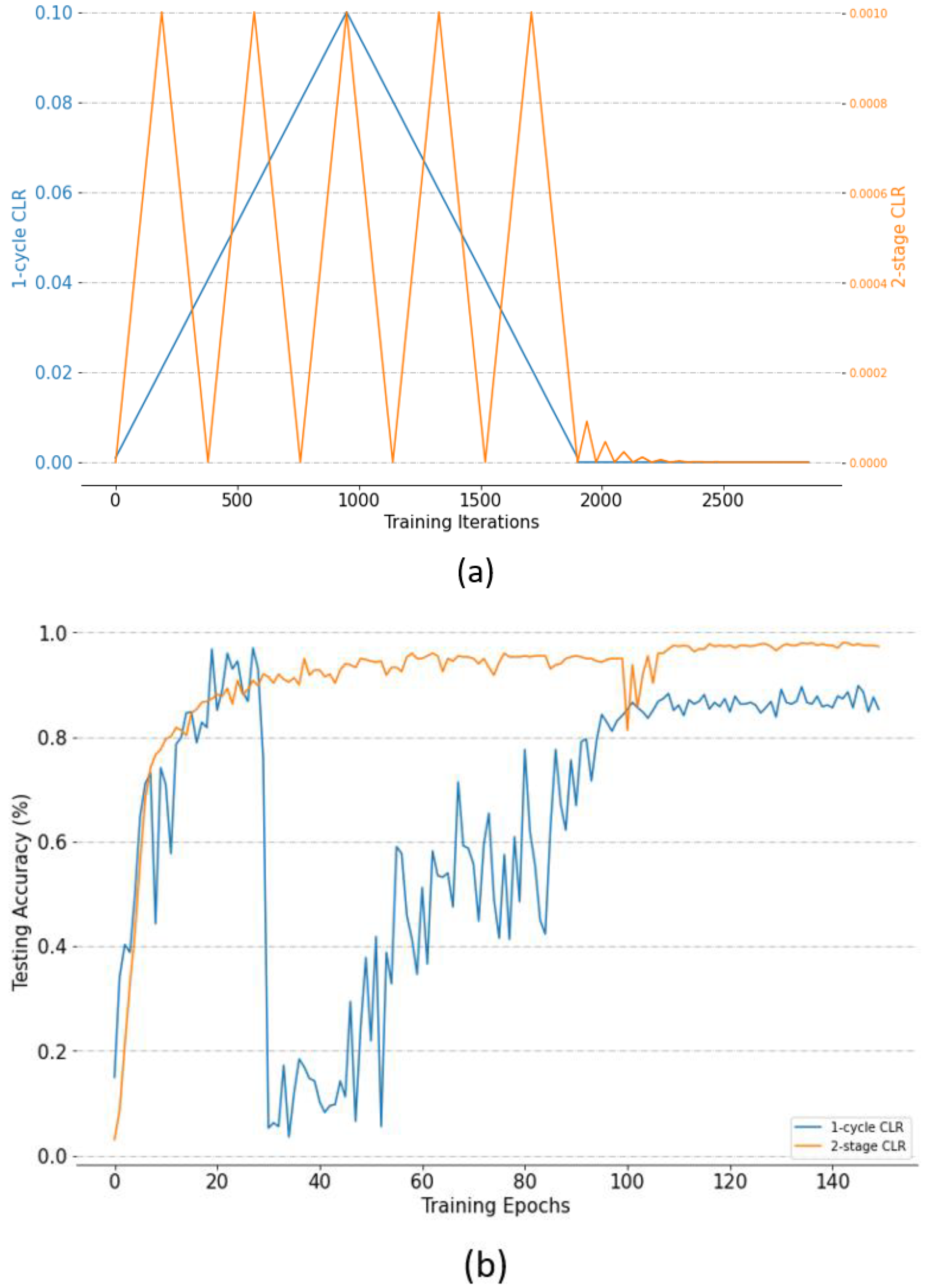
Different cyclical learning-rate methods

In this section, we compare the performances of the two-stage cyclical learning rate method (2-stage CLR, Figure 11) and Smith and Topin’s (2019) one-cycle cyclical learning rate method (1-cycle CLR). The results of Figure 12 showed that the two-stage cyclical learning rate method achieved the highest test accuracy of 98.0% at epoch = 134. On the contrary, the one-cycle cyclical learning rate method only achieved the highest test accuracy of 97.0% at epoch = 27. Although the latter could provide quicker access to the best test accuracy for training, the former could achieve a better test accuracy; hence, it was used in subsequent experimental results for model training and performance testing.

4.2.2. Experimental Results

1.

Classification of UC Merced land-use dataset

In this section, the classification results for the UC Merced land-use dataset are discussed. The t-SNE analysis method was used for the classification. This method is a non-linear dimensionality-reduction algorithm used for exploring high-dimensional data. It can map multi-dimensional data to two or more dimensions using technology suitable for visual presentation. In this study, extracting the features of the deep layers for analysis helped with the understanding of the differences between the features obtained by the model before and after training. In Figure 13a, which shows the results before training, the features extracted by the model show little correlation; however, after training, as shown in Figure 13b, the features are highly clustered, thus showing that these models do help to improve the classification performance.

Figure 14 shows the VGG16 model supplemented by the model classification matrix proposed in this study using the best classification weights obtained from the early training termination strategy. The resulting confusion matrix is also shown; the training rate was 80%. The matrix contains the individual classification results for 21 categories. The kappa coefficients of the UC Merced dataset were 0.9985 and 0.9895 at 80% and 50% training, respectively.

In

Table 1. Comparison of the overall accuracy and standard deviations using 80% and 50% training ratios on UC Merced dataset.

Method	80% Training Ratio	50% Training Ratio
GoogLeNet [33]	94.31 ± 0.89	92.70 ± 0.60
CaffNet [33]	95.02 ± 0.81	93.98 ± 0.67
VGG-16 [33]	95.21 ± 1.20	94.14 ± 0.69
salM3LBP-CLM [34]	95.75 ± 0.80	94.21 ± 0.75
CNN-R+VLAD with SVM [35]	95.85	NA
TEX-Net-LF [36]	96.62 ± 0.49	95.89 ± 0.37
VGG19+Hybrid-KCRC [37]	96.33	NA
Two-Stream Fusion [38]	98.02 ± 1.03	96.97 ± 0.75
CTFCNN [39]	98.44 ± 0.58	NA
GCFs + LOFs [32]	99.00 ± 0.35	97.37 ± 0.44
Inception-v3-CapsNet [40]	99.05 ± 0.24	97.59 ± 0.16
MVFLN+VGG-VD16 [41]	99.52 ± 0.17	NA
RSSCNet (this paper)	99.81 ± 0.06	98.76 ± 0.19

, the classification results found in this study are compared with those obtained using other classification methods. It can be seen that, by using the two-stage cyclical learning-rate training method, this study achieved the best overall accuracy out of the results shown.

2.

Classification of RSSCN7 dataset

The t-SNE analysis method was used to extract the deep features of the proposed model and to analyze it. In this section, the classification results obtained by applying this model to the RSSCN7 dataset are discussed. As shown in Figure 15b, after training, the features became highly clustered, which shows that the model proposed by this research helps to improve the scene classification.

Figure 16 shows the overall accuracy confusion matrix extracted by VGG16 supplemented by the classification method proposed in this study and using the optimal classification weights in the training early termination strategy. The training rate used was 50%. The matrix contains the individual classification results for seven categories. Among these, agricultural land and grassland are most likely to be confused. This is perhaps because the two categories have similar characteristics—both containing a large proportion of green ground, which easily leads to errors. The kappa coefficients of the RSSCN7 dataset were 0.9737 and 0.9329 at 50% and 20% training, respectively.

Table 2. Comparison of the overall accuracy and standard deviations using 50% and 20% training ratios on RSSCN7 dataset.

Method	50% Training Ratio	20% Training Ratio
DBN [20]	77.00	NA
GoogLeNet [33]	85.84 ± 0.92	82.55 ± 1.11
CaffNet [33]	88.25 ± 0.62	85.57 ± 0.95
VGG-16 [33]	87.18 ± 0.94	83.98 ± 0.87
Deep Filter Banks [42]	90.4 ± 0.6	NA
GCFs + LOFs [32]	95.59 ± 0.49	92.47 ± 0.29
RSSCNet (this paper)	97.41 ± 0.27	93.51 ± 0.51

shows a comparison of the results obtained for the RSSCN7 dataset classification using different recently proposed methods, including the one proposed in this paper. The proposed two-stage cyclical learning-rate training method achieved the best overall accuracy for two different training ratios. With a 50% training ratio, it produced an increase in accuracy of about 3% compared with other methods.

3.

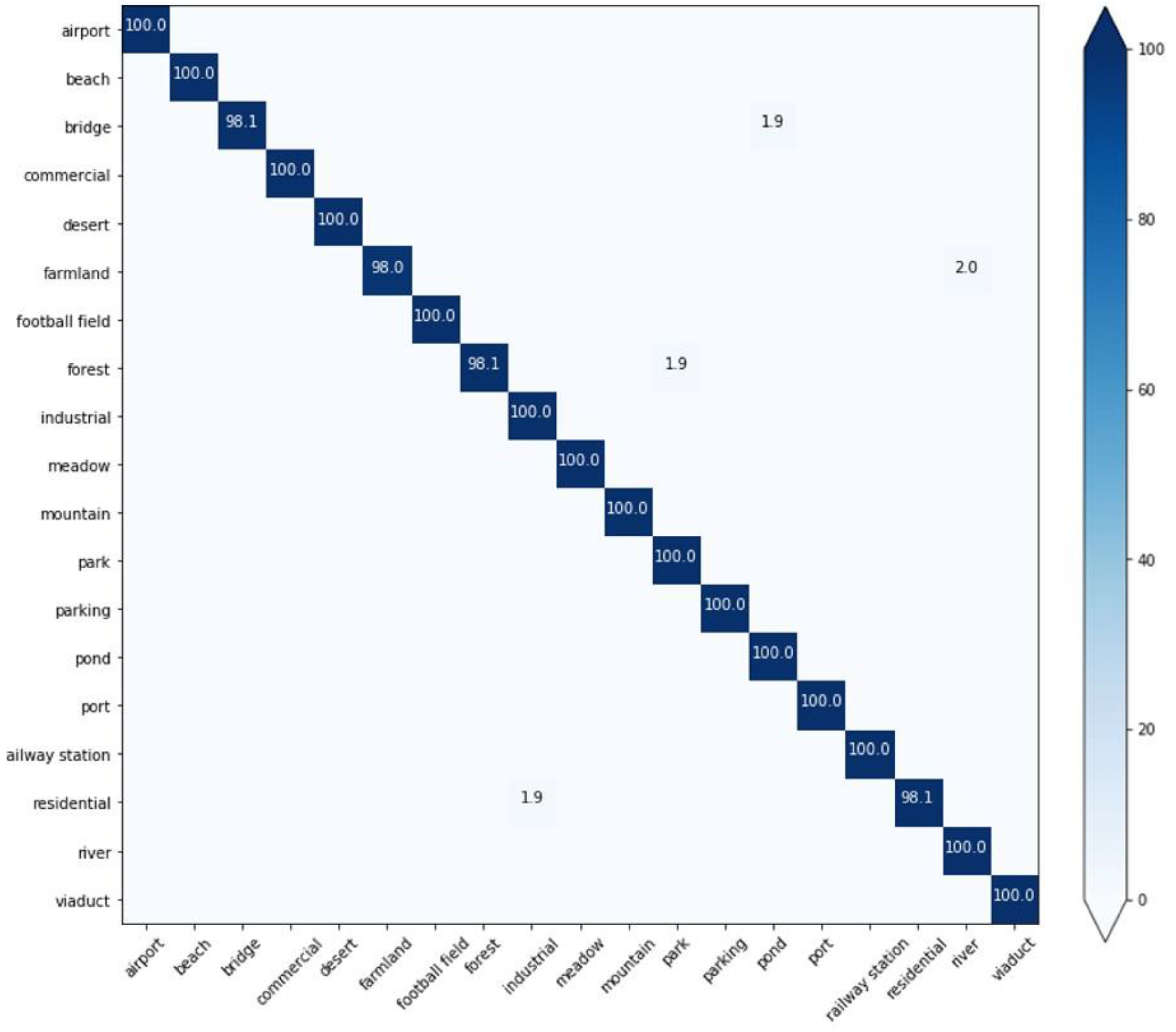
Classification of WHU-RS19 dataset

The t-SNE analysis method was used to extract the deep features of the proposed model and to analyze it. In this section, the classification results obtained by applying this model to the WHU-RS19 dataset are discussed. As shown in Figure 17b, as a result of the training, the features became highly clustered, showing that the proposed model helps to improve the classification of the scene.

Figure 18 shows the confusion matrix for the WHU-RS19 dataset extracted using VGG16 with the classification types proposed in this study and the optimal classification weights from the training early termination strategy. The training rate used was 60%. The matrix contains the individual classification results for the 19 categories in the dataset. Among these categories, the combinations football field and park and of forest and mountain were the most easily confused during the classification.

Table 3. Comparison of the overall accuracy and standard deviations using 60% and 40% training ratios on WHU-RS19 dataset.

Method	60% Training Ratio	40% Training Ratio
GoogLeNet [33]	94.71 ± 1.33	93.12 ± 0.82
CaffNet [33]	96.24 ± 0.56	95.11 ± 1.20
VGG-16 [33]	96.05 ± 0.91	95.44 ± 0.60
TEX-Net-LF [36]	98.00 ± 0.52	97.61 ± 0.36
Two-Stream Fusion [38]	98.92 ± 0.52	98.23 ± 0.56
RSSCNet (this paper)	99.46 ± 0.21	98.54 ± 0.37

shows a comparison between the results of the WHU-RS19 dataset classification obtained using the proposed method and methods proposed in other recent papers. Using the two-stage cyclical learning-rate training method proposed in this study, our proposed method achieved the best overall accuracy. The kappa coefficients of the WHU-RS19 dataset were 0.9968 and 0.9874 at 60% and 40% training, respectively.

From the confusion matrix classification results shown in Figure 18, it can be seen that the categories that are misclassified in the WHU-RS19 dataset include “residential”, “forest”, “farmland”, and “bridge” (Figure 19a). We first used the LIME analysis on the misclassified four images and generated the super-pixel feature regions that the model was most interested in (Figure 19b). By observing the super-pixel area in Figure 19b, we can understand why the model misclassifies “residential” as “industrial”, “forest” as “park”, “farmland” as “river”, and “bridge” as “pond”.

This research attempted to correct the four images misjudged by the model in Figure 19a with the hopes of improving the model classification performance. First, with regard to the reason for the wrong judgment of the “residential” image, we believe that the other images of the residential category in the dataset contained various bright colors as a whole, while the roofs of the buildings in industrial areas tended to be mostly white. The house colors tended to be white, which may have led to the classification errors. Therefore, the color of the “residential” image was increased in saturation to make it more similar to the other “residential” images in the dataset. From the super-pixel area of the “forest”, the cut block contained a part of the bare land, which was different from the other images in this category, which mostly only contained forests. The colors and the details were also blurred. Therefore, the color contrast was enhanced, the overall sharpness of the image was increased, the shadows between the trees were intensified, and the image was prevented from being judged as a “park” again. The image of the “farmland” depicts that the light of the horizontal road in the image is quite obvious, and a green straight line is included in the captured image features. Therefore, we reduced the brightness of the strong part of the image. In the “farmland” parts, we performed a small sharpening to try to remove the noise in the image and strengthen the details of the interval between farmlands. In the last “bridge” image, the feature did not contain the “bridge” feature at all. Therefore, we increased the brightness of the “bridge” itself and the color saturation and sharpness of the image. We also tried to increase the chance of a “bridge” edge being captured as a feature. Figure 20a,b present the four corrected images and their corresponding super-pixel feature regions, respectively. Finally, the four corrected images were replaced with the original images, and the category prediction of the entire dataset was again performed. Consequently, the result reached an overall accuracy of 100%. Figure 21 displays the corrected classification matrix.

4.2.3. Further Explanation and Discussion

In this section, we further discuss how fine-tuning, a circular learning rate, and an increase in the amount of data can improve the classification performance. The classification results obtained in this study can be expanded to help understand the possible impact of this project on model training.

1.

The effectiveness of fine-tuning

In Section 4 of this paper, two-stage training using the proposed model was described, and it was found that the proposed method has significant optimization for training. Moreover, we also wanted to understand, in addition to not carrying out freezing in the first stage, whether freezing the first 19 layers in the second stage would produce different results from those obtained by freezing different layers at two different stages. Therefore, we investigated three different situations: no freezing of any layer, freezing of the top seven layers, and freezing of top the 19 layers; the results for different combinations of these three situations are shown in Figure 22.

The five combinations investigated were no freezing at either stage (shown as “0 + 0”), top seven layers frozen at second stage only (“0 + 4”), top 13 layers frozen at second stage only (“0 + 13”), top 13 layers frozen at first stage only (“13 + 0”), and top 13 layers frozen at two stages (“13 + 13”). From Figure 22, it can be seen that two-stage training with no freezing (“0 + 0”) achieved the best testing accuracy. The test accuracy was the worst when the top 13 layers were frozen in the two training phases (“13 + 13”). According to the results of Figure 22, the test accuracy increases as the number of fine-tuning layers increases.

2.

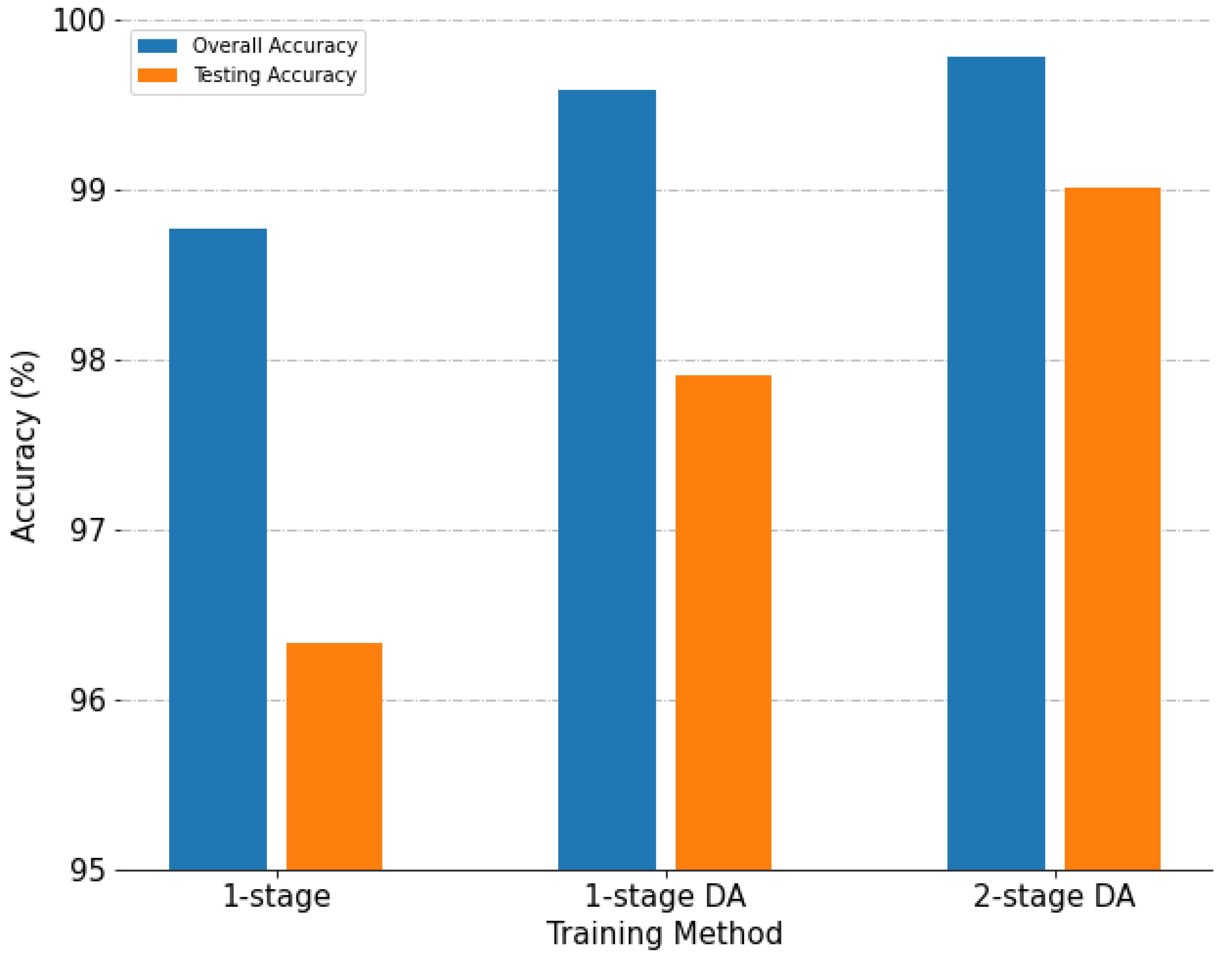
Effectiveness of image data augmentation

In this study, after inverting and increasing the number of images by carrying out a small amount of panning and zooming, augmentation training was also included in the training. As shown in Figure 23, doing this also successfully increased the training accuracy. The results here are shown as no data augmentation ((shown as “1-stage” in Figure 23), single-stage data augmentation included in the training (“1-stage DA”), and two-stage data augmentation included in the training (“2-stage DA”).

3.

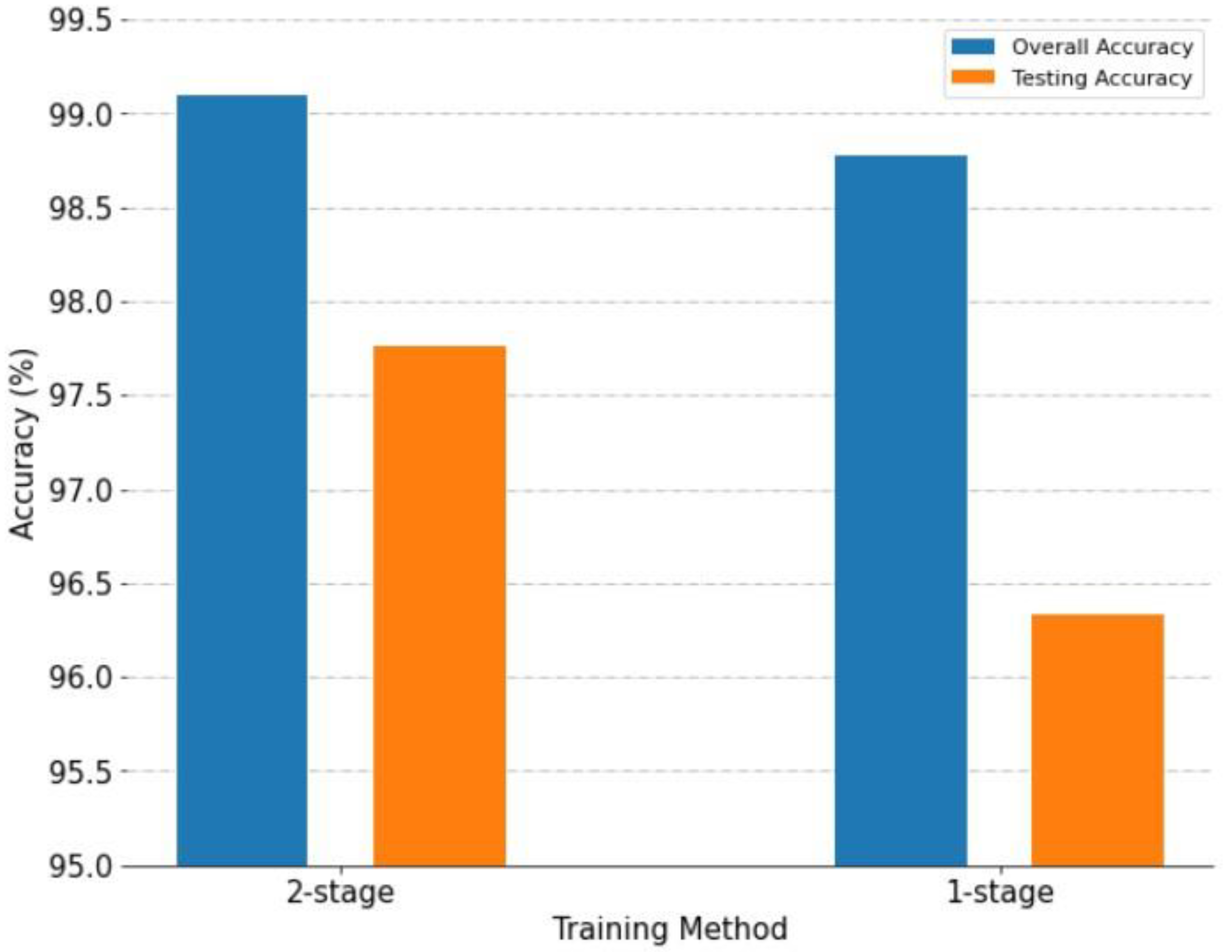
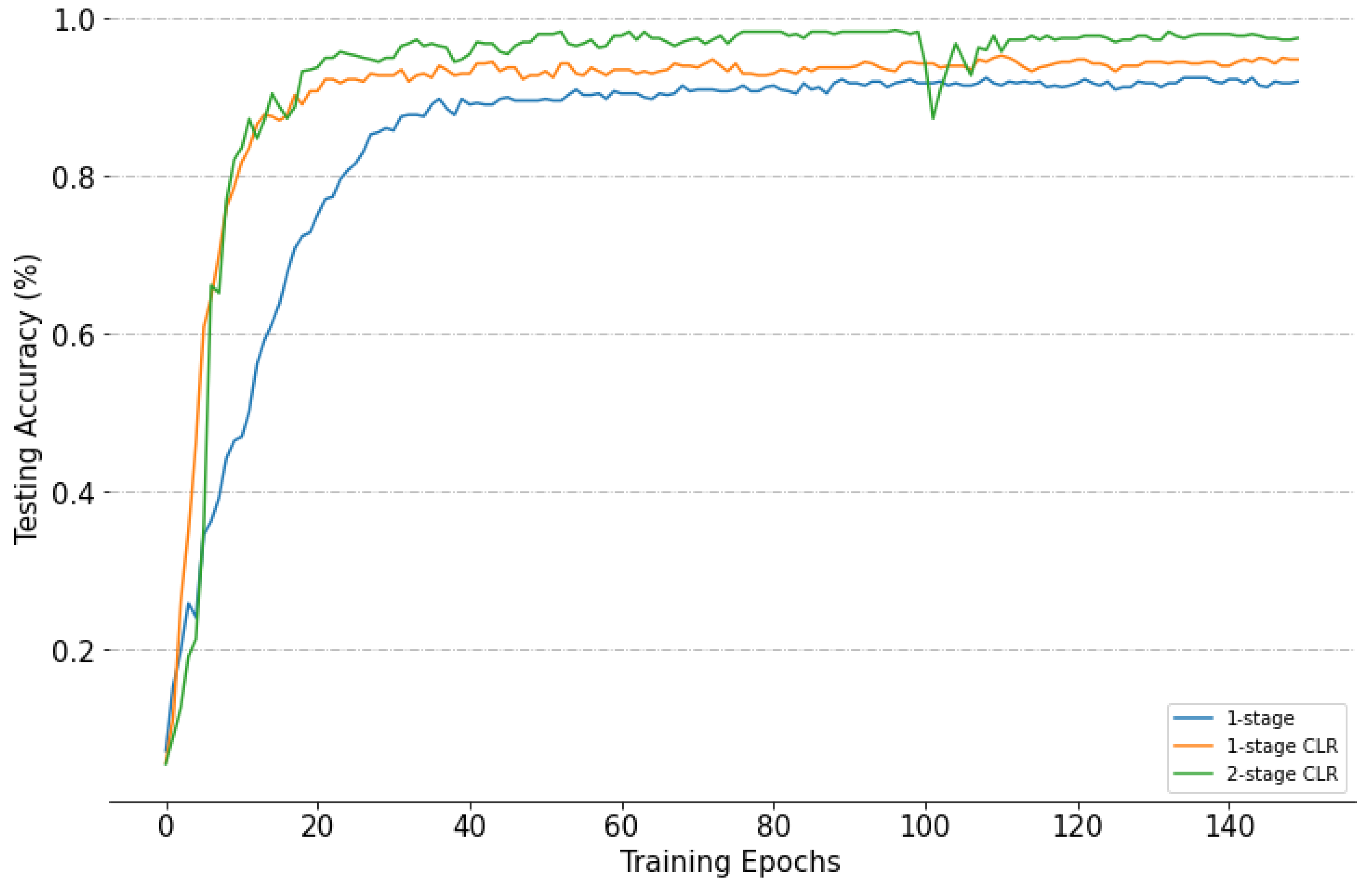
Effectiveness of using a two-stage cyclical learning-rate method

In two-stage cyclical learning, the training can be implemented using two different optimizers. In this study, an SGD optimizer with a cyclical learning rate was used in the first stage. In the second stage, an Adam optimizer was used for the training. In two-stage cyclical learning-rate training, this method obtains the best weight in the first stage and then enter the second stage. When used together with the cyclical learning rate, this can greatly accelerate the convergence. Figure 24 shows a comparison of the number of iterations needed to achieve the best level of accuracy for three different training methods.

When only a single-stage fixed learning rate (shown as “1-stage” in Figure 24) was used for the training, the convergence speed was the slowest and the lowest test accuracy was obtained. The use of a single-stage cyclical learning rate (“1-stage CLR”) could speed up the convergence and give a greater chance of avoiding the local optimal solution so that better results could be obtained. When a two-stage circular learning rate (“2-stage CLR”) was used in the early part of the second training stage, due to the change of optimizer, the process of finding the best accuracy fluctuated. However, overall, the best accuracy could be reached more quickly, using the smallest number of iterations of the three methods.

5. Conclusions

As a result of continued advances in technology, better-quality and higher-resolution data can be obtained, leading to improvements in remote sensing image classification and in predictions based on it. It takes a lot of time to train and adjust the classification. In order to reduce the time required for the training of the model and to explore how quickly the model can converge with high-generation capability, we recommend the RSSCNet model integrated with the simultaneous use of a two-stage cyclical learning-rate training policy and the no-freezing transfer learning technology that requires only a small number of iterations. In this way, an excellent level of accuracy can be obtained. Data augmentation technology, regularization, and early stopping strategy can then be used to also deal with the problem of limited generalization encountered in the rapid training of deep neural networks. The experimental results that were obtained also confirm that the use of the model and training strategies proposed in this paper can outperform current models in terms of accuracy.

In this study, by using the LIME super-pixel explanation, the root causes of model classification errors were made clearer and a better understanding was obtained. This made it easier to carry out subsequent processing and adjustment of the data or models. After the image correction preprocessing on the four misclassified images using the RSSCNet model in the WHU-RS19 dataset, this image correction procedure was found to improve the overall classification accuracy. This investigation is only a preliminary study.

In future research, we will try to establish universal image correction preprocessing for the case of suspected outliers and merge different XAI (explainable artificial intelligence) analysis technologies to improve interpretation capabilities so that they can be applied to a more diverse range of imagery with different classification issues.

References

1. Gu, Y.; Wang, Y.; Li, Y. A survey on deep learning-driven remote sensing image scene understanding: Scene classification, scene retrieval and scene-guided object detection. Appl. Sci. 2019, 9, 2110. [Google Scholar] [CrossRef] [Green Version]
2. Scholl, V.M.; Cattau, M.E.; Joseph, M.B.; Balch, J.K. Integrating national ecological observatory network (neon) airborne remote sensing and in-situ data for optimal tree species classification. Remote Sens. 2020, 12, 1414. [Google Scholar] [CrossRef]
3. Cheriyadat, A.M. Unsupervised feature learning for aerial scene classification. IEEE Trans. Geosci. Remote Sens. 2014, 52, 439–451. [Google Scholar] [CrossRef]
4. Mahdianpari, M.; Granger, J.E.; Mohammadimanesh, F.; Salehi, B.; Brisco, B.; Homayouni, S.; Gill, E.; Huberty, B.; Lang, M. Meta-analysis of wetland classification using remote sensing: A systematic review of a 40-year trend in north america. Remote Sens. 2020, 12, 1882. [Google Scholar] [CrossRef]
5. Luus, F.P.S.; Salmon, B.P.; Van den Bergh, F.; Maharaj, B.T.J. Multiview deep learning for land-use classification. IEEE Geosci. Remote Sens. Lett. 2015, 12, 2448–2452. [Google Scholar] [CrossRef] [Green Version]
6. Maire, F.; Mejias, L.; Hodgson, A. A convolutional neural network for automatic analysis of aerial imagery. In Proceedings of the 2014 International Conference on Digital Image Computing: Techniques and Applications (DICTA), Wollongong, New South Wales, Australia, 25–27 November 2014; pp. 1–8. [Google Scholar]
7. Wang, T.; Thomasson, J.A.; Yang, C.; Isakeit, T.; Nichols, R.L. Automatic classification of cotton root rot disease based on uav remote sensing. Remote Sens. 2020, 12, 1310. [Google Scholar] [CrossRef] [Green Version]
8. Tong, X.-Y.; Xia, G.-S.; Lu, Q.; Shen, H.; Li, S.; You, S.; Zhang, L. Land-cover classification with high-resolution remote sensing images using transferable deep models. Remote Sens. Environ. 2020, 237, 111322. [Google Scholar] [CrossRef] [Green Version]
9. Zhang, Z.; Jiang, R.; Mei, S.; Zhang, S.; Zhang, Y. Rotation-invariant feature learning for object detection in vhr optical remote sensing images by double-net. IEEE Access 2019, 8, 20818–20827. [Google Scholar] [CrossRef]
10. Zhong, Y.; Han, X.; Zhang, L. Multi-class geospatial object detection based on a position-sensitive balancing framework for high spatial resolution remote sensing imagery. ISPRS J. Photogramm. Remote Sens. 2018, 138, 281–294. [Google Scholar] [CrossRef]
11. Hu, F.; Xia, G.-S.; Hu, J.; Zhang, L. Transferring deep convolutional neural networks for the scene classification of high-resolution remote sensing imagery. Remote Sens. 2015, 7, 14680–14707. [Google Scholar] [CrossRef] [Green Version]
12. Nogueira, K.; Penatti, O.A.; dos Santos, J.A. Towards better exploiting convolutional neural networks for remote sensing scene classification. Pattern Recognit. 2017, 61, 539–556. [Google Scholar] [CrossRef] [Green Version]
13. Penatti, O.A.; Nogueira, K.; Dos Santos, J.A. Do deep features generalize from everyday objects to remote sensing and aerial scenes domains? In Proceedings of the IEEE Conference on Computer Vision and Pattern Recognition, Boston, MA, USA, 7–12 June 2015; pp. 44–51. [Google Scholar]
14. Smith, L.N. Cyclical learning rates for training neural networks. In Proceedings of the 2017 IEEE Winter Conference on Applications of Computer Vision (WACV), Santa Rosa, CA, USA, 24–31 March 2017; pp. 464–472. [Google Scholar]
15. Smith, L.N.; Topin, N. Super-convergence: Very fast training of neural networks using large learning rates. In Proceedings of the Artificial Intelligence and Machine Learning for Multi-Domain Operations Applications, Baltimore, MD, USA, 10 May 2019; p. 1100612. [Google Scholar]
16. Leclerc, G.; Madry, A. The two regimes of deep network training. arXiv 2020, arXiv:2002.10376. [Google Scholar]
17. Caruana, R.; Lawrence, S.; Giles, C.L. Overfitting in neural nets: Backpropagation, conjugate gradient, and early stopping. In Proceedings of the Advances in Neural Information Processing Systems, Cambridge, MA, USA, 2001; pp. 402–408. [Google Scholar]
18. Sheng, G.; Yang, W.; Xu, T.; Sun, H. High-resolution satellite scene classification using a sparse coding based multiple feature combination. Int. J. Remote Sens. 2012, 33, 2395–2412. [Google Scholar] [CrossRef]
19. Yang, Y.; Newsam, S. Bag-of-visual-words and spatial extensions for land-use classification. In Proceedings of the 18th SIGSPATIAL International Conference on Advances in Geographic Information Systems, San Jose, CA, USA, 2–5 November 2010; pp. 270–279. [Google Scholar]
20. Zou, Q.; Ni, L.; Zhang, T.; Wang, Q. Deep learning based feature selection for remote sensing scene classification. IEEE Geosci. Remote Sens. Lett. 2015, 12, 2321–2325. [Google Scholar] [CrossRef]
21. Simonyan, K.; Zisserman, A. Very deep convolutional networks for large-scale image recognition. arXiv 2014, arXiv:1409.1556. [Google Scholar]
22. Perez, H.; Tah, J.H.; Mosavi, A. Deep learning for detecting building defects using convolutional neural networks. Sensors 2019, 19, 3556. [Google Scholar] [CrossRef] [PubMed] [Green Version]
23. Clevert, D.-A.; Unterthiner, T.; Hochreiter, S. Fast and accurate deep network learning by exponential linear units (elus). arXiv 2015, arXiv:1511.07289. [Google Scholar]
24. Ioffe, S.; Szegedy, C. Batch normalization: Accelerating deep network training by reducing internal covariate shift. arXiv 2015, arXiv:1502.03167. [Google Scholar]
25. Shorten, C.; Khoshgoftaar, T.M. A survey on image data augmentation for deep learning. J. Big Data 2019, 6, 60. [Google Scholar] [CrossRef]
26. Maaten, L.V.D.; Hinton, G. Visualizing data using t-sne. J. Mach. Learn. Res. 2008, 9, 2579–2605. [Google Scholar]
27. Linderman, G.C.; Rachh, M.; Hoskins, J.G.; Steinerberger, S.; Kluger, Y. Fast interpolation-based t-sne for improved visualization of single-cell rna-seq data. Nat. Methods 2019, 16, 243–245. [Google Scholar] [CrossRef] [PubMed]
28. Song, W.; Wang, L.; Liu, P.; Choo, K.-K.R. Improved t-sne based manifold dimensional reduction for remote sensing data processing. Multimed. Tools Appl. 2019, 78, 4311–4326. [Google Scholar] [CrossRef]
29. Ribeiro, M.T.; Singh, S.; Guestrin, C. “Why should I trust you?” Explaining the predictions of any classifier. In Proceedings of the 22nd ACM SIGKDD International Conference on Knowledge Discovery and Data Mining, San Francisco, CA, USA, 13–17 August 2016; pp. 1135–1144. [Google Scholar]
30. He, K.; Zhang, X.; Ren, S.; Sun, J. Deep residual learning for image recognition. In Proceedings of the IEEE Conference on Computer Vision and Pattern Recognition, Las Vegas, NV, USA, 27–30 June 2016; pp. 770–778. [Google Scholar]
31. Szegedy, C.; Vanhoucke, V.; Ioffe, S.; Shlens, J.; Wojna, Z. Rethinking the inception architecture for computer vision. In Proceedings of the IEEE Conference on Computer Vision and Pattern Recognition, Las Vegas, NV, USA, 27–30 June 2016; pp. 2818–2826. [Google Scholar]
32. Zeng, D.; Chen, S.; Chen, B.; Li, S. Improving remote sensing scene classification by integrating global-context and local-object features. Remote Sens. 2018, 10, 734. [Google Scholar] [CrossRef] [Green Version]
33. Xia, G.-S.; Hu, J.; Hu, F.; Shi, B.; Bai, X.; Zhong, Y.; Zhang, L.; Lu, X. Aid: A benchmark data set for performance evaluation of aerial scene classification. IEEE Trans. Geosci. Remote Sens. 2017, 55, 3965–3981. [Google Scholar] [CrossRef] [Green Version]
34. Bian, X.; Chen, C.; Tian, L.; Du, Q. Fusing local and global features for high-resolution scene classification. IEEE J. Sel. Top. Appl. Earth Obs. Remote Sens. 2017, 10, 2889–2901. [Google Scholar] [CrossRef]
35. Li, P.; Ren, P.; Zhang, X.; Wang, Q.; Zhu, X.; Wang, L. Region-wise deep feature representation for remote sensing images. Remote Sens. 2018, 10, 871. [Google Scholar] [CrossRef] [Green Version]
36. Anwer, R.M.; Khan, F.S.; van de Weijer, J.; Molinier, M.; Laaksonen, J. Binary patterns encoded convolutional neural networks for texture recognition and remote sensing scene classification. ISPRS J. Photogramm. Remote Sens. 2018, 138, 74–85. [Google Scholar] [CrossRef] [Green Version]
37. Liu, B.-D.; Xie, W.-Y.; Meng, J.; Li, Y.; Wang, Y. Hybrid collaborative representation for remote-sensing image scene classification. Remote Sens. 2018, 10, 1934. [Google Scholar] [CrossRef] [Green Version]
38. Yu, Y.; Liu, F. A two-stream deep fusion framework for high-resolution aerial scene classification. Comput. Intell. Neurosci. 2018, 2018, 8639367. [Google Scholar] [CrossRef] [Green Version]
39. Huang, H.; Xu, K. Combing triple-part features of convolutional neural networks for scene classification in remote sensing. Remote Sens. 2019, 11, 1687. [Google Scholar] [CrossRef] [Green Version]
40. Zhang, W.; Tang, P.; Zhao, L. Remote sensing image scene classification using cnn-capsnet. Remote Sens. 2019, 11, 494. [Google Scholar] [CrossRef] [Green Version]
41. Guo, Y.; Ji, J.; Shi, D.; Ye, Q.; Xie, H. Multi-view feature learning for vhr remote sensing image classification. Multimed. Tools Appl. 2020. [Google Scholar] [CrossRef]
42. Wu, H.; Liu, B.; Su, W.; Zhang, W.; Sun, J. Deep filter banks for land-use scene classification. IEEE Geosci. Remote Sens. Lett. 2016, 13, 1895–1899. [Google Scholar] [CrossRef]
Figure 1. Example images of UC Merced dataset: (a) agriculture; (b) airplane; (c) baseball diamond; (d) beach; (e) buildings; (f) chaparral; (g) dense residential; (h) forest; (i) freeway; (j) golf course; (k) harbor; (l) intersection; (m) medium residential; (n) mobile home park; (o) overpass; (p) parking lot; (q) river; (r) runway; (s) sparse residential; (t) storage tanks; (u) tennis court.
Applsci 10 06151 g001
Figure 2. Example images of RSSCN7 dataset: (a) grass; (b) field; (c) industry; (d) river lake; (e) forest; (f) resident; (g) parking.
Applsci 10 06151 g002
Figure 3. Example images of WHU-RS19 dataset: (a) airport; (b) beach; (c) bridge; (d) commercial; (e) desert; (f) farmland; (g) football field; (h) forest; (i) industrial; (j) meadow; (k) mountain; (l) park; (m) parking; (n) pond; (o) port; (p) railway station; (q) residential; (r) river; (s) viaduct.
Applsci 10 06151 g003
Figure 4. Convolutional neural network model.
Applsci 10 06151 g004
Figure 5. CNN classifier network architecture of our RSSCNet model.
Applsci 10 06151 g005
Figure 6. Cyclical learning rate during training.
Applsci 10 06151 g006
Figure 7. Image explanation using LIME (local interpretable model, agnostic explanation): (a) example of correct classification; (b) misclassified example.
Applsci 10 06151 g007
Figure 8. Comparison of accuracy using different pre-trained models.
Applsci 10 06151 g008
Figure 9. Comparison of accuracy using different fine-tuning layers.
Applsci 10 06151 g009
Figure 10. Comparison of overall accuracy with and without two-stage training.
Applsci 10 06151 g010
Figure 11. Comparison of testing accuracy using different classification architectures.
Applsci 10 06151 g011
Figure 12. Comparison of testing accuracy using different cyclical learning rate (CLR) methods: (a) cyclical learning-rate policy; (b) testing accuracy.
Applsci 10 06151 g012
Figure 13. Visual analysis on UC Merced dataset using t-distributed stochastic neighbor embedding (t-SNE): (a) before training; (b) after training.
Applsci 10 06151 g013
Figure 14. Classification confusion matrix of our method on UC Merced dataset.
Applsci 10 06151 g014
Figure 15. Visual analysis on RSSCN7 dataset using t-SNE: (a) before training; (b) after training.
Applsci 10 06151 g015
Figure 16. Classification confusion matrix of our method on RSSCN7 dataset.
Applsci 10 06151 g016
Figure 17. Visual analysis on WHU-RS19 dataset using t-SNE: (a) before training; (b) after training.
Applsci 10 06151 g017
Figure 18. Classification confusion matrix of our method on WHU-RS19 dataset.
Applsci 10 06151 g018
Figure 19. Misclassified images on WHU-RS19 dataset: (a) original image; (b) super-pixel explanation by LIME analysis.
Applsci 10 06151 g019
Figure 20. After correction of misclassified images on WHU-RS19 dataset: (a) corrected image; (b) super-pixel explanation by LIME analysis.
Applsci 10 06151 g020
Figure 21. Classification confusion matrix of WHU-RS19 dataset after image correction.
Applsci 10 06151 g021
Figure 22. Overall accuracy of fine-tuning using different frozen combinations.
Applsci 10 06151 g022
Figure 23. Accuracy of different training methods.
Applsci 10 06151 g023
Figure 24. Test accuracy of with and without two-stage cyclical learning-rate method.
Applsci 10 06151 g024