Probing Collisional Plasmas with MCRS: Opportunities and Challenges

Abstract

Since the 1940s, Microwave Cavity Resonance Spectroscopy (MCRS) has been used to investigate a variety of solids, gases, and low-pressure plasmas. Recently, the working terrain of the diagnostic method has been expanded with atmospheric-pressure plasmas. This review discusses the advancements that were required for this transition and implications of studying highly collisional, with respect to the probing frequencies, plasmas. These developments and implications call for a redefinition of the limitations of MCRS, which also impact studies of low-pressure plasmas using the diagnostic method. Moreover, a large collection of recommendations concerning the approach and its potential for future studies is presented.

1. Introduction

Since the introduction of Microwave Cavity Resonance Spectroscopy (MCRS) as a plasma diagnostic in the 1940s [1], the technique has been solidified by a series of publications [2,3,4,5]. Over the last eight decades, the measurement approach has been used to study various types of low-pressure plasmas: pristine radio-frequency (RF) driven low-pressure plasmas [6,7], powder-forming plasmas [8,9,10], etching plasmas [11], ultracold plasmas [12], and extreme ultraviolet photon-induced plasmas [13,14,15]. The measurement approach has also been used to determine properties of materials, i.e., dielectric constants [16] and molar polarizations [17]. A giant leap in this development of the diagnostic tool was the introduction of the multi-mode approach, which enabled resolving spatial distributions of the electron density in low-pressure plasmas [14]. In the exemplary applications of MCRS as plasma diagnostic mentioned above, the change in the spectral position of a resonance peak of an electromagnetic standing wave in a plasma-filled cavity was used to determine the changes in permittivity that subsequently were related to the electron density $n_{\mathrm{e}}$ of the cavity’s content.

Only recently has it been demonstrated that MCRS can be used to study the electron dynamics between successive discharges in an atmospheric-pressure pulsed plasma jet in N${}_2$ feed gas [18]. In such atmospheric-pressure discharges, the contributions of the electron density $n_{\mathrm{e}}$ and the electron momentum transfer collision frequency ${\nu }_{\mathrm{m}}$ to the alterations in the complex permittivity $\tilde{\epsilon }$ need to be separated. The changes in the position as well as the width of a resonance peak were used to separate and determine the individual contributions. This ‘atmospheric-pressure’ avenue was continued by exploring the full temporal evolution of electron dynamics in the spatial afterglow of an RF-driven atmospheric-pressure plasma jet [19]. In both investigations of these atmospheric-pressure discharges, the changes in resonant behavior were relatively small and for this reason, the resolution in permittivity had to be improved significantly over the last few years.

As the resolution of MCRS improved, more phenomena could be probed with the method. This is because the presence of free electrons is only one of the factors affecting the resonant behavior. The importance of separating the different contributors to changes in the resonant behavior during plasma experiments was demonstrated in the study of an RF plasma jet [20]. In that work, the contributions of the plasma dynamics, the acoustic waves, and most likely the gas composition were separated.

In contrast to most MCRS studies of low-pressure plasmas, the investigated atmospheric-pressure plasmas did not occupy the whole cavity volume. The electric field profile of the resonant mode and the volume occupied by the plasma were determined in order to correct for the partially-filled cavity. This procedure currently limits the determination of the effective plasma volume, which is the plasma volume weighted by the electric-field-squared, and subsequently the obtained electron density, to its order of magnitude [18].

With the transition towards probing atmospheric-pressure plasmas, the perspective on the limitations of the diagnostic method has changed and the description of the limitations needs to be adapted. The first meticulous theoretical investigation of the validity of the MCRS diagnostic method has been performed by Persson [21]. Unfortunately, the limitations were not presented in an accessible way which reduced the impact of the work. Agdur et al. [22] have focused on the perturbation of the resonant field by the plasma and derived an analytical expression for the resonance frequency of a partially-filled cavity.

The practical limit ${\omega }_{\mathrm{pe}}$ ≪ $\omega$ is most often used to indicate the maximum measurable electron density [23,24,25,26]. Here, ${\omega }_{\mathrm{pe}}$ denotes the electron plasma frequency—which depends on the electron density—and $\omega$ the angular frequency of the applied microwave field. Above this limit, the shift of the resonance frequency no longer scales linearly with the increase in the electron density and translating measurements into tangible physical parameters becomes difficult. However, this limit underestimates the range of plasma parameters that can be explored by MCRS. Especially for atmospheric-pressure plasmas—which do not fill the whole cavity volume and have a collision frequency larger than the angular microwave frequency—a new and more accurate limit would be beneficial for opening up an extension of the dynamic range of applicability of the diagnostic technique. A simpler approach is the usage of the (collisional) skin depth as an additional parameter to limit the range of plasmas, which can be probed by MCRS [18,25], but this condition also does not capture all relevant physics involved. Several theoretical studies have been performed to investigate the perturbation of the microwave field by the presence of the plasma [22,27,28,29]. Experiments demonstrated that overdense plasmas (${\omega }_{\mathrm{pe}}$ > $\omega$) can be probed when the plasma is located at a node of the applied resonant field [24]. Furthermore, the non-linear regime of the response of a cavity has been used to investigate discharges [28]. Besides sufficient spectral resolution, i.e., resolution in changes in permittivity, the resonant field needs to be able to respond to the changes in the probing volume [30].

This review article presents an overview of the opportunities and challenges in this new field for MCRS. The presented challenges needed to be overcome or taken into account during the preparation and execution of the experiments described in references [18,19,20]. Moreover, there are several complicators in the analysis of experimental data related to atmospheric- and low-pressure plasmas. As these challenges could have a severe impact on the outcome of the analysis, it is necessary to propound them. These ‘warnings’ will often be accompanied by (possible) solutions. First, the general concepts of MCRS and the relevant physics are introduced in Section 2. The main messages of this article are related to the required improvement of the resolution, contributors to changes in resonant behavior, inhomogenous plasmas, determination of the effective plasma volume, lower limit for the permittivity, and the skin depth of the plasma. Each of the six main messages will be covered in one of the Section 3.1, Section 3.2, Section 3.3, Section 3.4, Section 3.5 and Section 3.6. This all is followed by a collection of recommendations to take (new) users of this diagnostic method by the hand as well as to suggest further improvements of the approach itself. The article is finalized with a conclusion.

2. Theory

2.1. Resonant Behavior of a Standing Microwave

A standing wave—also referred to as a stationary wave—is a wave of which the nodes and antinodes do not move in space over time. Examples of this phenomenon can be found in, e.g., the oscillation of a drum’s membrane and that of a guitar’s string.

The Microwave Cavity Resonance Spectroscopy method is based on the physical principle that the resonant behavior of an electromagnetic standing wave in a hollow space—the cavity—surrounded by a metal structure depends on the permittivity $\epsilon$ and permeability $\mathsf{\mu }$ of the cavity volume. The computed spatial profile of the electric field amplitude $\left|E\right|$ of the fundamental resonant mode (i.e., TM${}_{010}$) in a cylindrical cavity is shown in Figure 1.

The standing wave in a cavity is typically excited by microwaves via an antenna that protrudes only slightly into this cavity. A typical frequency response of a cavity (red marks) is shown in Figure 2. From a response like this, the resonant behavior, i.e., the spectral position and the width of the resonance peak, is determined by optimized fitting algorithms (blue line).

The spectral position of a resonance peak does not only depend on the material properties $\epsilon$ and $\mathsf{\mu }$ but also on the dimensions of the cavity and the excited resonant mode. Typical frequencies used for MCRS as a plasma diagnostic are 1–10 GHz [7,9,31]. The cavity is only able to absorb microwaves when the applied frequency matches the resonance frequency $f_{\mathrm{res}}$ ($f=\omega {/}_{2\pi }$) of a probed resonant mode. This frequency can be found by locating the spectral position where the least power is reflected.

The second property of the resonant behavior is the width of a resonance peak, which is proportional to the losses in the cavity. The losses and width of a specific mode are indicated by the quality factor Q (or in short ‘Q’) [32],

$$Q\equiv \frac{f_{\mathrm{res}}}{\mathsf{\Gamma }},$$

(1)

where $\mathsf{\Gamma }$ is the Full-Width-at-Half-Maximum (FWHM) of the peak (the frequency and power axes need to be in linear scale). When the losses in a cavity are high, the resonant mode is able to respond fast to changes inside the cavity volume. The characteristic time $\tau$ of a resonant mode is given by:

$$\tau =\frac{Q}{\pi f_{\mathrm{res}}}.$$

(2)

This 1/e response time is used to indicate the time it takes for the resonant field to adapt 63% to a new situation. For this reason, it takes a few $\tau$ for the field to ‘fully’ adapt to, e.g., a sudden presence of plasma. Typical values in experiments for $\tau$ vary from ∼0.01 to 1 $\mathsf{\mu }$s.

The temporal resolution of the diagnostic technique is fundamentally limited by the fact that forming a standing wave requires a number of passes of the electromagnetic waves in the cavity. The quality factor of a resonant mode is a good indication for this number of passes. The technological limitations related to the temporal resolution are the rise and fall times of the microwave power detector and the sampling frequency of the microwave power detector’s output.

2.2. Perturbations

As mentioned before, the properties of the material inside the cavity volume $V_{\mathrm{cav}}$ affect the resonant behavior of the excited standing wave. The change in the resonance frequency $\Delta f$ ($\Delta f$ = $f_2-f_1$) and the change in the reciprocal Q-factor $\Delta \left(\frac{1}{Q}\right)$ ($\Delta \left(\frac{1}{Q}\right)$ = $\frac{1}{Q_2}-\frac{1}{Q_1}$) are described by the following relation [18,33],

$$\frac{\Delta f}{f_1}+i\frac{1}{2}\Delta \left(\frac{1}{Q}\right)=-\frac{{\displaystyle {\int \int \int }_{V_{\mathrm{cav}}}\left(\Delta \tilde{\epsilon }\left(\mathbf{r}\right)|{\mathbf{E}}_1{\left(\mathbf{r}\right)|}^2+\Delta \tilde{\mu }\left(\mathbf{r}\right){\left|{\mathbf{H}}_1\left(\mathbf{r}\right)\right|}^2\right)d^3\mathbf{r}}}{{\displaystyle 2{\epsilon }_0{\int \int \int }_{V_{\mathrm{cav}}}{\left|{\mathbf{E}}_1\left(\mathbf{r}\right)\right|}^2{d}^3\mathbf{r}}},$$

(3)

where the subscript 1 is used for the unperturbed cavity and 2 for the perturbed state, i the imaginary unit number, ${\mathbf{E}}_1$ the local electric field of the resonant mode of the unperturbed cavity, ${\mathbf{H}}_1$ the local magnetic field of the resonant mode of the unperturbed cavity, $\mathbf{r}$ the position vector, and ${\epsilon }_0$ the vacuum permittivity. The local change of the complex permittivity $\Delta \tilde{\epsilon }$ is given by:

$$\Delta \tilde{\epsilon }\left(\mathbf{r}\right)={\tilde{\epsilon }}_2\left(\mathbf{r}\right)-{\tilde{\epsilon }}_1\left(\mathbf{r}\right),$$

(4)

where ${\tilde{\epsilon }}_1$ and ${\tilde{\epsilon }}_2$ are the complex permittivity of the unperturbed and perturbed cavity, respectively. The derivation of this equation can be found in reference [18]. In this derivation, it is assumed that the resonant field profile is not disturbed by the perturbation and that $f_1$ ≈ $f_2$.

In this work, it is assumed that the plasma is unmagnetized, i.e., $\tilde{\mu }$ = ${\mathsf{\mu }}_0$ ([34], p. 109), where ${\mathsf{\mu }}_0$ is the vacuum permeability. Hence, Equation (3) can be simplified by $\Delta \tilde{\mu }$ = 0.

By separating the real and imaginary parts of Equation (3), the contributors to changes in f and $\frac{1}{Q}$ are separated,

$$\frac{\Delta f}{f_1}=-\frac{{\displaystyle \Re \left({\int \int \int }_{V_{\mathrm{cav}}}\Delta \tilde{\epsilon }\left(\mathbf{r}\right){\left|{\mathbf{E}}_1\left(\mathbf{r}\right)\right|}^2{d}^3\mathbf{r}\right)}}{{\displaystyle 2{\epsilon }_0{\int \int \int }_{V_{\mathrm{cav}}}{\left|{\mathbf{E}}_1\left(\mathbf{r}\right)\right|}^2{d}^3\mathbf{r}}},$$

(5)

$$\Delta \left(\frac{1}{Q}\right)=-\frac{{\displaystyle \Im \left({\int \int \int }_{V_{\mathrm{cav}}}\Delta \tilde{\epsilon }\left(\mathbf{r}\right){\left|{\mathbf{E}}_1\left(\mathbf{r}\right)\right|}^2{d}^3\mathbf{r}\right)}}{{\displaystyle {\epsilon }_0{\int \int \int }_{V_{\mathrm{cav}}}{\left|{\mathbf{E}}_1\left(\mathbf{r}\right)\right|}^2{d}^3\mathbf{r}}}.$$

(6)

These equations show that the method is most sensitive in the regions where the strength of the resonant field is largest. To be more exact, the material properties obtained by this integral from MCRS are cavity volume averaged and weighted with the square of the local electric field.

Another type of perturbation is a change in the dimensions or shape of the cavity, e.g., due to thermal expansion of the metal structure which surrounds the cavity. For low-pressure plasmas, this is not of major importance because the effect is relatively small. However, the investigated atmospheric-pressure plasmas [18,19] induce a change in resonance frequency which can be similar to that caused by a temperature increase of ∼10 mK and therefore this mechanism can no longer be neglected.

A third type of perturbation is related to changes in the impedance of the conducting walls surrounding the cavity. The change in the surface reactance leads to, among other things, a ‘virtual’ change in the dimensions of the cavity due to a change in the skin depth. The importance of this effect when probing plasmas is investigated in Section 3.2.2. A more detailed description of the wall-impedance perturbation can be found in ([35], p. 255).

2.3. Plasma’s Permittivity

The Drude–Lorentz model is commonly used to describe the complex permittivity of a plasma ${\tilde{\epsilon }}_i$ as [34],

$${\tilde{\epsilon }}_i={\epsilon }_0\left[{\tilde{\epsilon }}_{\mathrm{r},\mathrm{gas},i}-\frac{{\omega }_{\mathrm{pe}}^2}{{\nu }_{\mathrm{m}}^2+4{\pi }^2{f}^2}-i\frac{{\nu }_{\mathrm{m}}}{\omega }\frac{{\omega }_{\mathrm{pe}}^2}{{\nu }_{\mathrm{m}}^2+4{\pi }^2{f}^2}\right],$$

(7)

where ${\epsilon }_{\mathrm{r},\mathrm{gas},i}$ is the relative permittivity of the gas and is traditionally assumed to be unity, ${\nu }_{\mathrm{m}}$ the momentum transfer collision frequency of the electrons, and f the frequency of the applied electromagnetic field. The electron plasma frequency ${\omega }_{\mathrm{pe}}$ is given by [34]:

$${\omega }_{\mathrm{pe}}=\sqrt{\frac{n_{\mathrm{e}}{e}^2}{{\epsilon }_0{m}_{\mathrm{e}}}},$$

(8)

where $n_{\mathrm{e}}$ is the electron density, e the elementary charge, and $m_{\mathrm{e}}$ the electron mass. One of the assumptions in the Drude–Lorentz model is that the collision cross section does not depend on the energy of the electrons, and this is generally not true. In two of our works [18,19] an effective collision frequency is used to circumvent this problem.

The following two equations for $\Delta f/f_1$ and $\Delta \left(\frac{1}{Q}\right)$ are obtained by substituting Equation (7) into Equations (5) and (6) while assuming ${\tilde{\epsilon }}_{\mathrm{r},\mathrm{gas},1}$ = ${\tilde{\epsilon }}_{\mathrm{r},\mathrm{gas},2}$ and $n_{\mathrm{e}}$ = 0 m${}^{-3}$ for the unperturbed state,

$$\frac{\Delta f}{f_1}=\frac{e^2}{2{\epsilon }_0{m}_{\mathrm{e}}}\frac{{\displaystyle {\int \int \int }_{V_{\mathrm{cav}}}\frac{n_{\mathrm{e}}\left(\mathbf{r}\right)}{{\nu }_{\mathrm{m}}^2\left(\mathbf{r}\right)+4{\pi }^2{f}_2^2}{\left|{\mathbf{E}}_1\left(\mathbf{r}\right)\right|}^2{d}^3\mathbf{r}}}{{\displaystyle {\int \int \int }_{V_{\mathrm{cav}}}{\left|{\mathbf{E}}_1\left(\mathbf{r}\right)\right|}^2{d}^3\mathbf{r}}},$$

(9)

$$\Delta \left(\frac{1}{Q}\right)=\frac{e^2}{2\pi {\epsilon }_0{m}_{\mathrm{e}}{f}_1}\frac{{\displaystyle {\int \int \int }_{V_{\mathrm{cav}}}\frac{n_{\mathrm{e}}\left(\mathbf{r}\right){\nu }_{\mathrm{m}}\left(\mathbf{r}\right)}{{\nu }_{\mathrm{m}}^2\left(\mathbf{r}\right)+4{\pi }^2{f}_2^2}{\left|{\mathbf{E}}_1\left(\mathbf{r}\right)\right|}^2{d}^3\mathbf{r}}}{{\displaystyle {\int \int \int }_{V_{\mathrm{cav}}}{\left|{\mathbf{E}}_1\left(\mathbf{r}\right)\right|}^2{d}^3\mathbf{r}}}.$$

(10)

As an example, in a radio-frequency driven plasma at 10 Pa, the collision frequency ${\nu }_{\mathrm{m}}$ = 0.2 GHz ([36], p. 5) which is much smaller than the probing frequencies and can, therefore, be neglected. A typical collision frequency in an atmospheric-pressure plasma jet is ∼1 THz [37], which is significant with respect to the resonance frequencies used in MCRS experiments. In this case, the role of the collisions of the electrons is very important and must, therefore, be included in the analysis of MCRS experiments. So far only the temporal and spatial afterglow of atmospheric-pressure plasmas were investigated with MCRS [18,19]. In these studies, the capability of MCRS to probe highly collisional plasmas with collision frequencies up to 0.5 THz was demonstrated [18]. In the literature, no MCRS studies of the bulk—in which the electron temperature and collision frequency of the electrons are higher than in the afterglows—of an atmospheric-pressure plasma are described. Figure 3 presents the change in the real and imaginary part of the relative permittivity with respect to ${\epsilon }_{\mathrm{r},\mathrm{gas}}$ as a function of the electron density for f = 3.5 GHz and a variety of collision frequencies. For ${\nu }_{\mathrm{m}}$ = 0 Hz, the imaginary part of the relative permittivity is zero and is, therefore, not visible in this logarithmic plot in Figure 3b. Both graphs show that for increasing collision frequencies the change in the real part and in the imaginary part decreases.

Note that in this work collisional plasma denotes a plasma in which the momentum transfer collision frequency of the electrons ${\nu }_{\mathrm{m}}$ is not much smaller than the angular frequency $\omega$ of the applied microwave field. This definition might differ from the one used in other works.

2.4. Non-Collisional Plasmas

In most low-pressure plasmas the collision frequency ${\nu }_{\mathrm{m}}$ is much smaller than the angular microwave frequencies $\omega$ for typical cavities, and therefore the dissipation term—the imaginary part—in Equation (7) can be neglected. Advantageous for the low-pressure case is that it does not require information concerning the losses of the resonant field to obtain the electron density because the electron collision frequency can be assumed zero. Hence, Equation (9) can be reduced to,

$$\frac{\Delta f}{f_1}=\frac{e^2}{8{\epsilon }_0{m}_{\mathrm{e}}{\pi }^2{f}_2^2}\frac{{\displaystyle {\int \int \int }_{V_{\mathrm{cav}}}{n}_{\mathrm{e}}\left(\mathbf{r}\right){\left|{\mathbf{E}}_1\left(\mathbf{r}\right)\right|}^2{d}^3\mathbf{r}}}{{\displaystyle {\int \int \int }_{V_{\mathrm{cav}}}{\left|{\mathbf{E}}_1\left(\mathbf{r}\right)\right|}^2{d}^3\mathbf{r}}}.$$

(11)

In most prior MCRS experiments, the equation has been even further simplified,

$$\frac{\Delta f}{f_1}=\frac{e^2{\overline{n}}_{\mathrm{e}}}{8{\epsilon }_0{m}_{\mathrm{e}}{\pi }^2{f}_2^2},$$

(12)

which can be rewritten into [9,15,38,39],

$$\begin{array}{c}\hfill {\overline{n}}_{\mathrm{e}}=\frac{8{\epsilon }_0{m}_{\mathrm{e}}{\pi }^2{f}_2^2}{e^2}\frac{\Delta f}{f_1}.\end{array}$$

(13)

Here, ${\overline{n}}_{\mathrm{e}}$ is the cavity averaged and electric-field-squared weighted electron density given by:

$$\begin{array}{c}\hfill {\overline{n}}_{\mathrm{e}}=\frac{{\displaystyle {\int \int \int }_{V_{\mathrm{cav}}}{n}_{\mathrm{e}}\left(\mathbf{r}\right){\left|{\mathbf{E}}_1\left(\mathbf{r}\right)\right|}^2{d}^3\mathbf{r}}}{{\displaystyle {\int \int \int }_{V_{\mathrm{cav}}}{\left|{\mathbf{E}}_1\left(\mathbf{r}\right)\right|}^2{d}^3\mathbf{r}}}.\end{array}$$

(14)

2.5. Collisional Plasmas

For experiments in which the collisions of the electrons with neutrals cannot be neglected, the position and width of a resonance peak are used to separate the contributions of the electron density and collision frequency to the real and imaginary part of the permittivity. Atmospheric-pressure plasmas are typically significantly smaller than the cavity and a completely filled cavity can therefore not be assumed. In this case the volume occupied by the plasma needs to be determined by, for example, camera images.

The atmospheric-pressure plasmas investigated in references [18,19] were assumed to have no spatial dependency within the plasma volume. With this assumption, the collision frequency of the electrons ${\nu }_{\mathrm{m}}$ is given by [18,23],

$$\begin{array}{c}\hfill {\nu }_{\mathrm{m}}=\pi f_1\frac{\Delta (1/Q)}{\Delta f/f_1},\end{array}$$

(15)

while the electron density $n_{\mathrm{e}}$ can be obtained from [18,23],

$$\begin{array}{c}\hfill n_{\mathrm{e}}=\frac{2{\epsilon }_0{m}_{\mathrm{e}}}{e^2}\frac{{\nu }_{\mathrm{m}}^2+4{\pi }^2{f}_1^2}{\mathcal{V}}\frac{\Delta f}{f_1}.\end{array}$$

(16)

Here, $\mathcal{V}$ is the ratio between the effective (electric-field-squared weighted) plasma volume and the effective (electric-field-squared weighted) cavity volume,

$$\mathcal{V}=\frac{{\int \int \int }_{V_{\mathrm{p}}}{\left|{\mathbf{E}}_1\right|}^2{d}^3\mathbf{r}}{{\int \int \int }_{V_{\mathrm{cav}}}{\left|{\mathbf{E}}_1\right|}^2{d}^3\mathbf{r}}.$$

(17)

In contrast to in the derivation of Equation (13), the influence of the change in resonance frequency on the permittivity of the plasma is not taken into account in Equations (15) and (16). The influence of the assumption of no spatial dependency on the results of investigations of plasma with a spatial profile in the electron dynamics is investigated in Section 3.3.

A disadvantage of probing a plasma with an electron collision frequency that is much higher than the probing frequencies is that the relative shift in resonance frequency $\Delta f/f_1$ is much smaller than would be the case for a non-collisional plasma with the same electron density. For a $f_{\mathrm{res}}$ of 3.5 GHz, the $\Delta f/f_1$ is ∼2100 times smaller for a plasma with a ${\nu }_{\mathrm{m}}$ of 1 THz compared to that with a ${\nu }_{\mathrm{m}}$ = 0 Hz. Furthermore, $\mathcal{V}$ ≪ 1 for atmospheric-pressure plasmas, which reduces $\Delta f/f_1$ even more. These atmospheric-pressure plasmas typically have a higher electron density which compensates (partially) for the two mechanisms described above. However, for the atmospheric-pressure discharges investigated in our articles [18,19]$\Delta f/f_1$ has been ∼4 orders of magnitude smaller than that for typical low-pressure plasmas.

2.6. Examples of Prior Studies of Collisional Plasmas

To give an impression of typical MCRS results obtained while studying collisional plasmas, two prior studies of atmospheric-pressure plasma jets are discussed. In the first study [19] the electron dynamics of the spatial afterglow of a radio-frequency driven atmospheric-pressure plasma jet and in the second study [20] acoustic waves produced by such a jet were investigated. A schematic overview of the experimental setup used in both studies is presented in Figure 4. Plasma was created by applying an RF voltage on the central needle electrode with respect to the cylindrical shell-shaped grounded electrode. Between these electrodes, a helium gas flow was present which was (partially) ionized by the electric field between the electrodes. As MCRS is a differential measurement scheme, it requires periods in which no plasma is present for the measurement to be successful. For this reason, the plasma was produced for short periods, i.e., 50 $\mathsf{\mu }$s in these experiments, with a repetition rate $f_{\mathrm{rep}}$.

For the MCRS measurements, a cylindrical microwave cavity with a resonance frequency $f_{\mathrm{res}}$ of 3.5 GHz for the TM${}_{010}$ mode was used. This mode had a quality factor of $Q=4\times {10}^3$ and provided a temporal resolution of ∼1 $\mathsf{\mu }$s. The gas flow and discharge were able to enter and exit the cavity via concentric holes of 13 mm in diameter in the top and bottom flat walls. A microwave generator was used to create the probing signal with power $P_{\mathrm{in}}$ (1 mW) at frequency $f=\omega /2\pi$. The microwaves travelled via a directional coupler to a straight antenna that protruded a few mm into the cavity. Ten percent of the reflected microwaves travelled via the directional coupler to a logarithmic power detector of which the output was sampled at 10 MHz using a transient recorder. To synchronize this sampling procedure with the discharges, the recorder and RF power delivery system were triggered by a pulse/delay generator. As the discharge dynamics were extremely reproducible, it was allowed to use multiple discharges to create a spectral response for each time step and to reduce noise by averaging. Setting the applied microwave frequency and saving the data of the transient recorder was done by in-house developed software.

2.6.1. Electron Dynamics

During the period in which RF power was supplied to the needle electrode and the 100 $\mathsf{\mu }$s directly after the plasma pulse, the electron dynamics were assumed to be the dominant contributors to the changes in resonant behavior [19]. The shift of the normalized resonance frequency $\Delta f/f_1$ and the changes in the reciprocal quality factor $\Delta (1/Q)$ are shown in Figure 5a,b, respectively. As the plasma did not fill the whole cavity, it was necessary for the analysis to determine the plasma occupied volume and calculate the electric field profile (see Figure 6). The data of this simulation was used in Equation (17) to calculate $\mathcal{V}\approx 1.7\times {10}^{-6}$. This parameter and the temporal data of $\Delta f/f_1$ and $\Delta (1/Q)$ were used to calculate the electron density $n_{\mathrm{e}}$ and ${\nu }_{\mathrm{eff}}$ presented in Figure 5c,d.

2.6.2. Acoustic Waves

After the plasma had decayed, phenomena other than the electron dynamics still affected the response of the cavity as was shown in the second study [20]. A moving average over the data was used—although at the cost of temporal resolution—to increase the resolution in changes in the permittivity further. The change in the relative resonance frequency $\Delta f/f_1$ as a function of time for a $f_{\mathrm{rep}}$ of 62.5 Hz is shown in Figure 7a. In a subsequent data processing step, the data related to the period where electron dynamics contributed significantly to the response was removed. The remaining data were used to calculate the required pressure difference to induce the determined shift in resonance frequency. In Figure 7b, the magenta line presents the required pressure difference in He to cause the response of the cavity. The cyan line indicates the data for helium after a second moving average with a cutoff frequency of 3.7 kHz. This effect was attributed to changes in the He/air ratio within the cavity volume. By subtracting these low-frequency components from the original signal, the contributions of the acoustic waves could be separated. Figure 8 presents the evolution of acoustic waves caused by gas heating by the plasma.

2.7. Brief Summary

By resolving the changes in resonant behavior of an electromagnetic standing wave, properties of the material inside the cavity volume and the cavity itself can be determined. For most low-pressure plasmas, it is sufficient to measure the change in the spectral position of a resonance peak. However, with the transition towards probing atmospheric-pressure plasmas, the change of the peak’s width also becomes equally relevant. Moreover, these collisional plasmas induce much smaller changes in the resonance frequency and therefore require a very good resolution in monitoring the resonant behavior. One of the disadvantages of studying plasmas that only induce a very small change in resonant behavior is that it requires to take a large variety of physical phenomena into account, which can affect the measurements and separating these contributions is not trivial.

3. Results and Discussion

3.1. Increased Accuracy in the Permittivity

The high collisionality of the electrons in atmospheric-pressure plasmas suppresses the change in the real part of the permittivity, which is responsible for the shift in $f_{\mathrm{res}}$. Hence, an increase in the accuracy of the determination of the resonance frequency was required for the transition towards probing atmospheric-pressure plasmas. The typical resolution in the change in the relative permittivity is $\sim {10}^{-3}-{10}^{-5}$ [9,13,39,40]. However, a resolution of $\sim {10}^{-7}$ is reported in exceptional cases [7,41,42]. This value means that the standard deviation in the resonance frequency is less than 1-part-per-5-billion. In this article, we present an increase of the resolution in the real part of the permittivity by more than two orders of magnitude to $\sim 4\times {10}^{-10}$ with respect to these works. This improvement in resolution has been made possible by replacing the trusted transmission scheme [8,31,43,44,45] by measurements in reflection mode [14], improving the fitting algorithm [18], increasing the number of averages [15,18,19], increasing the number of probing frequencies [15,18,19], improving the mechanical stability of the cavity [19], introducing temperature-corrected apparent frequencies [19], and temporal averaging [15,20]. To the best of the authors’ knowledge, the resolution in the quality factor has not been specified earlier. In this article, the best accuracy in $\Delta (1/Q)$ was ∼10${}^{-6}$.

In this section, the influence of the number of averages and the frequency step size on the error of the determined resonance frequency and quality factor is covered to help other users of the diagnostic method to optimize the total duration of the experiment. The cavity—and the rest of the setup—used for this study is described in detail in reference [19] and had a $f_{\mathrm{res}}$ of 3.51 GHz and a Q of 4$\times {10}^3$ for the TM${}_{010}$ mode. The experiment was performed frequency-resolved with 4096 averages of the temporal responses per probing frequency and a frequency step size of 1 kHz over a range of 3.5075 to 3.5175 GHz. A typical spectral response for the TM${}_{010}$ mode of the cavity is shown in Figure 2.

The characteristic time $\tau$ of the used resonant mode was ∼0.36 $\mathsf{\mu }$s. This means that only 0.4 % of the resonant field was still remnant after 2 $\mathsf{\mu }$s and that measurements with these intervals were assumed to be uncoupled. Within each temporal response, 100 uncoupled samples were obtained. Due to a technical limitation, the maximum sample interval of 100 ns was shorter than the response time of the cavity. For this reason, the duration of each temporal response for a single frequency was 200 $\mathsf{\mu }$s and contained 2000 samples while only 1 in 20 subsequent samples in the temporal response were used in the analyses.

During the analyses, subsets of the experimental data were selected and used to emulate experiments for a range of frequency step sizes and a number of averages. The results presented here were obtained while 1 SLM He flow was passing through the cavity and were very similar to the results obtained without flow. In both experimental conditions, no discharges were produced. Note that in the past a larger standard deviation has been observed in experiments with flow compared to cases without flow. However, this problem has been solved by simultaneously improving the mechanical stability of the metal structure forming the cavity and its mounting.

For comparative purposes, the coefficient of variation ${\widehat{C}}_{\mathrm{v}}$ of each emulated experiment is computed,

$${\widehat{C}}_{\mathrm{v}}=\frac{s}{\overline{x}},$$

(18)

where s is the standard deviation and $\overline{x}$ the mean of the parameter of interest.

Figure 9 presents a graph in which ${\widehat{C}}_{\mathrm{v}}$ is indicated as a function of the frequency step size and the number of averages. The data related to $\Delta f$ is indicated in blue while red is used for $\Delta (1/Q)$. Squares are used for the parameter study with respect to the number of averages with a fixed frequency step size of 1 kHz, circles are used for the study with respect to the frequency step size with 4096 averaged temporal responses per probing frequency, and triangles are used for the complete data set with the maximum number of averages and frequencies (including temporal averaging with a width of 2 $\mathsf{\mu }$s). The total duration of the experiment was approximately 4 h, whereas the top horizontal axis indicates how much shorter the measurement time would have been for the emulated settings. Note, that the reduction factor is idealized by neglecting, e.g., the time it takes to adjust the probing frequency on the microwave generator and to save the measurement data.

The used approach was significantly less accurate in determining the Q of a resonant mode than the resonance frequency. This is not unexpected because Q contained the error in $f_{\mathrm{res}}$ in the first order and more importantly the procedure for the determination of FWHM was less accurate. However, this exercise shows that the accuracy could be improved by increasing the number of averages and probing frequencies in an experiment. Other avenues to increase the accuracy will be given in Section 4.

3.1.1. Size of Frequency Step vs. Number of Averages

Averaging of multiple measurement samples is a routine commonly used to reduce noise in experimental results. According to theory, the noise reduction follows $N^{\mathsf{\beta }}$, where N is the number of samples and $\mathsf{\beta }$ the exponent which indicates the noise reduction. In this experiment, N is the number of probing frequencies multiplied by the number of averages and if applicable multiplied by the sample width of the moving average. In the ideal case $\mathsf{\beta }$ = 0.5 [46]. Hereof in this section, the exponent $\mathsf{\beta }$ as a function of the frequency step size and number of averages is investigated.

In terms of this experiment, the exponent $\mathsf{\beta }$ is expressed as,

$$\frac{{\widehat{C}}_{\mathrm{v},\mathrm{high}}}{{\widehat{C}}_{\mathrm{v},\mathrm{low}}}={\left(\frac{N_{\mathrm{high}}}{N_{\mathrm{low}}}\right)}^{\mathsf{\beta }},$$

(19)

where ${\widehat{C}}_{\mathrm{v},\mathrm{low}}$ and ${\widehat{C}}_{\mathrm{v},\mathrm{high}}$ are the coefficient of variation for the experiment with the least samples and the most samples, respectively, and similarly for the number of samples $N_{\mathrm{low}}$ and $N_{\mathrm{high}}$.

Figure 10 presents a graph in which $\mathsf{\beta }$ is shown as a function of the experimental settings. The emulated experiment with 4096 averages and 1 kHz step size is used as a reference to compare the other settings to.

For very small frequency step sizes, $\mathsf{\beta }$ is lower than 0.5 and, more importantly, lower than the equivalent $\mathsf{\beta }$ for the scan of the number of averages. Despite that a parameter scan is only performed along the orthogonal axes of the parameter space, the results presented in this graph strongly indicate that it is best to reduce the number of probing frequencies over the width of the peak to ∼50, i.e., a frequency step size of 200 kHz while the remaining budget in measurement time can be used for probing additional discharges to increase the number of averages.

The exponent $\mathsf{\beta }$ for the scan of the number of averages fluctuates around 0.5. It can be concluded that the noise is reduced as expected for stationary noise with a mean which is zero [46]. It appears that the resolution in Q and $f_{\mathrm{res}}$ scales in the same manner with the sample size. The spread in the exponent $\mathsf{\beta }$ related to the number of averages decreases for the decreasing number of averages. This can be explained by the principle that the noise becomes smaller when the difference in sample size becomes larger.

The triangular symbols indicate the exponent related to the increase in resolution by the post-processing step in which 20 subsequent samples of $f_{\mathrm{res}}$ and Q were averaged. It appears that the reduction of noise by this method is less efficient than that by including additional samples as a result of probing more discharges. However, this moving average is relatively cheap in measurement time as it does not require additional discharges. Note that an increase in the sampling frequency to accommodate the moving average could lead to a longer duration of the experiment as more data needs to be saved. It is also important to mention that a moving average acts as a low-pass filter. Hence, it increases the ‘tardiness’ of the response of the cavity.

3.1.2. Influence of the Quality Factor

There is a trade-off between temporal resolution and spectral resolution in $f_{\mathrm{res}}$ considering a fixed amount of measurement time. A resonant mode that can respond fast has a broad peak and finding the spectral position of a wide peak accurately is more difficult than finding that of a narrow peak. The characteristic time $\tau$ of a resonant mode is proportional to the width of the peak and therefore to the error in the position. In the previous paragraph, it was shown that the error in the determination of the permittivity decreases with $N^{0.5}$. For this reason, the duration of an experiment scales inverse quadratically with the change in temporal resolution while maintaining the same resolution in $f_{\mathrm{res}}$.

In the description above, it is assumed that the position of the resonance frequency barely changes. This is true for experiments at atmospheric pressure as discussed in references [18,19,20]. However, in experiments in which the shift of the resonance frequency is significant—with respect to the width of a peak—temporal resolution becomes less expensive. A hand waving argument for this is to accommodate an increase in temporal resolution, the Q must decrease, which causes the peak to widen. As the ideal number of probing frequencies over the width of a peak is fixed, the total number of probing frequencies within the frequency range over which the resonance peak shifts decreases.

The resolution in Q does not change with a change in Q as long as the number of probed frequencies within the width of a peak is kept constant. However, in the analysis, the parameter $\Delta (1/Q)$ is used and the resolution of $\Delta (1/Q)$ is better for high Q. For small changes in Q, the resolution in $\Delta (1/Q)$ is inversely proportional to Q.

A very important property is the prominence of a resonance peak, i.e., the depth which is determined by the efficiency of the coupling of the microwaves into the cavity. Experimentally, a coupling of at least 10 dB appeared to be required to obtain decent results.

3.2. Contributors to Changes in the Resonant Behavior

The resonant behavior of a standing wave is influenced by perturbations in the cavity volume and changes related to the walls surrounding the cavity volume. As the resolution in resonant behavior of the diagnostic method has significantly increased over the last years, the diagnostic method is now sensitive enough to measure an extended range of phenomena. The different contributors to changes in the properties in the volume of the cavity are discussed in the section below and thereafter the influence of the temperature of the cavity walls is covered.

3.2.1. Contributors to Perturbations in the Cavity

The improvement of the resolution of MCRS in measuring changes in the permittivity made it possible to probe a range of processes that were previously out-of-range. Examples of this expanded functionality are the detection of acoustic waves and small changes in gas composition [20]. These contributions were separated from the electron dynamics and each other by deploying filters in the time and frequency domain. However, this required, due to the complexity, an extensive understanding of the investigated processes.

Some of the other properties that could be probed (non-selectively) are the temperature of the gas, thermal expansion of materials, humidity, position and shape of an item, gas flow fluctuations, oxidation processes, vapour in walls, bulk density of particles in the air, structure of materials, and water density [47,48]. Indirectly, MCRS could resolve information concerning photon energies, photon fluxes, ionization cross sections, magnetic fields, diffusion properties [1,13,14,15,49], radioactive decay, etc.

The electron density and permittivity are macroscopic material properties and with the improved detection limit presented in this article an electron density of only ∼0.1 mm${}^{-3}$ can be resolved. With the typical dimensions of the cavity, electron densities as such may no longer be described by macroscopic properties. Moreover, the collection of electrons and ions may no longer be a plasma.

Furthermore, with the improved resolution, the background ionization level may no longer be neglected. For example, changes in the temperature of the electrons could lead to anomalies like negative shifts as discussed in reference [49].

All the properties discussed above are related to the permittivity. However, with the recently developed very high resolution in the resonant behavior, it might be that the assumption of no change in the permeability is no longer valid.

3.2.2. Influence of the Cavity Walls’ Temperature

Temperature-corrected apparent frequencies are introduced to compensate for thermal expansion of the cavity [19]. This apparent frequency $f_{\mathrm{ap}}$, which is derived in Appendix A, is given by:

$$f_{\mathrm{ap}}\left(T_{\mathrm{cav}}\right)=\frac{f}{1+\alpha (T_{\mathrm{cav}}-T_0)},$$

(20)

where f is the applied microwave frequency, $\alpha$ the thermal expansion coefficient of the cavity’s wall material, $T_{\mathrm{cav}}$ the temperature of the walls during the measurement set with the same probing frequency f, and $T_0$ a fixed temperature for the whole measurement set. In reference [19], the temperature of the cavity was measured with ∼1 mK resolution for each set of temporal responses with the same probing frequency. In the analysis of the measurement data, the probing frequency is corrected for temperature fluctuations. The correction in frequency for thermal expansion of copper ($\alpha$ = $16.5\times {10}^{-6}$ K${}^{-1}$ [50]) walls—as used in reference [19]—is approximately 58 kHz/K. For a similar cavity surrounded by aluminium ($\alpha$ = $23.1\times {10}^{-6}$ K${}^{-1}$ [50]) as used in reference [18] the size of the correction is ∼81 kHz/K. Although the introduction of temperature-corrected apparent frequencies is a step forward, the approach does not correct for changes in the conductance $\sigma$ of the cavity’s walls due to variations in $T_{\mathrm{cav}}$ which affects the width as well as the position of the peak. The two responsible mechanisms for this dependency are treated below.

The first mechanism is related to the Ohmic losses in the cavity’s walls and is explored by an experiment. A vector network analyzer and the metal structure surrounding the cavity described in reference [18] were used to investigate the influence of its temperature on the quality factor of the TM${}_{010}$ resonant mode. A temperature-stabilized box was used to control the temperature of the cavity. Note that in this box the temperature of the gas was used to control $T_{\mathrm{cav}}$ and consequently also the permittivity of the gas was unintentionally changed [17].

Figure 11 presents a graph of the obtained Q as a function of $T_{\mathrm{cav}}$ and a linear fit through the measurement data.

The error bars in the figure represent the standard deviation in the determined Q in the set of measurements for the same temperature. The derivative of the fit $\frac{\Delta Q}{\Delta T_{\mathrm{cav}}}$ = −0.8 translates into a $\Delta (1/Q)$ of ∼$3\times {10}^{-7}$ for a temperature difference of 1 K. This is one order of magnitude below the best lower-detection limit for $\Delta (1/Q)$ as presented in Section 3.1.

Although this mechanism is below the detection limit for the determination of the changes in the imaginary part of the permittivity of our previous studies [18,19] for small temperature variations, it might still affect the determination of $f_{\mathrm{res}}$. To estimate the extent of this effect, the change in the distance from the resonance frequency to the spectral position of the frequency corresponding to the Full-Width-at-Half-Maximum (FWHM) is investigated. This spectral distance equals the difference in half of the FWHM. The change in the FWHM $\Delta \mathrm{FWHM}$ due to a change in $T_{\mathrm{cav}}$ from 300 to 301 K is expressed via Equation (1) as,

$$\Delta \mathrm{FWHM}=f_{\mathrm{res}}\left(\frac{1}{Q_{301\mathrm{K}}}-\frac{1}{Q_{300\mathrm{K}}}\right),$$

(21)

where $Q_{301\mathrm{K}}$ and $Q_{300\mathrm{K}}$ are the fitted values of the quality factor for the temperatures 301 and 300 K, respectively. In this example and for this position in the peak, the correction term of the spectral position $\frac{\Delta \mathrm{FWHM}}{2\Delta T_{\mathrm{cav}}}$ should be ∼0.5 kHz/K. Although this effect is measurable, it is significantly smaller than the correction term of several tens of kHz/K due to thermal expansion of the cavity walls. Hence, the complex relationship between the change in the width of the peak and quality factor is not taken into account. The complexity of correcting for this effect lies in the fact that the correction term of the probed frequency depends on the spectral distance to the resonance frequency. Due to the frequency-resolved measurement approach used in the experiments at atmospheric pressure [18,19,20], it is very difficult to determine the spectral distance because the data in a spectral response for a single time step is obtained with variations in the temperature of the cavity.

The other mechanism in which the conductance $\sigma$ of the wall influences the response of a cavity is via the skin depth of the resonant field into the metal walls, which makes the cavity appear to be a bit bigger for the microwaves than the physical dimensions of the cavity. The magnitude of this mechanism is estimated for the TM${}_{010}$ resonant mode and the setup used in reference [18]. The skin depth $\delta$ is expressed as [51],

$$\delta =\sqrt{\frac{\rho }{\pi f_{\mathrm{res}}{\mu }_0{\mu }_{\mathrm{r}}}},$$

(22)

where $\rho$ is the resistivity ($\rho =1/\sigma$) and ${\mathsf{\mu }}_{\mathrm{r}}$ the relative permeability, which is 1.000022 for aluminium [52].

The resistivity $\rho$ of aluminium [50] is used and interpolated in order to calculate the skin depth for 300 K and 301 K. The difference in $\delta$ between the two temperatures is ∼3 nm, which translates into a $\frac{\Delta f_{\mathrm{res}}}{\Delta T_{\mathrm{cav}}}$ of 0.3 kHz/K assuming the microwaves penetrate a single skin depth into the opposing walls on both sides. Hence, also the change in resonant behavior due to the alteration of skin depth is much smaller than the effect that thermal expansion induces on the resonant behavior. However, this effect is also well within the measurement range with the renewed resolution discussed in Section 3.1.

To recapitulate, a change in the temperature of the metal structure surrounding the cavity affects the resonant behavior in three ways: thermal expansion of the cavity, widening of the peak due to Ohmic losses, and a change of the skin depth making the cavity ‘virtually’ larger. Thermal expansion of the cavity’s walls appeared to be the dominant process and is, therefore, the only mechanism that is taken into account in the temperature-corrected apparent frequencies. Please be aware that for different wall materials and dimensions of the cavity itself, the extent of each of these contributions should be reconsidered.

3.3. Inhomogenous Plasmas

For plasmas with a spatial dependency of the plasma parameters, there is a fundamental challenge in disentangling the contributions of $n_{\mathrm{e}}$ and ${\nu }_{\mathrm{m}}$ to the changes in the cavity volume averaged complex permittivity $\tilde{\epsilon }$. This paragraph discusses the factors that impede the separation of these plasma properties.

When low-pressure plasmas are investigated, MCRS yields a cavity volume averaged electric-field-squared-weighted electron density ${\overline{n}}_{\mathrm{e}}$. This parameter is defined as follows [14,39],

$${\overline{n}}_{\mathrm{e}}=\frac{{\displaystyle {\int \int \int }_{V_{\mathrm{p}}}{n}_{\mathrm{e}}\left(\mathbf{r}\right){\left|{\mathbf{E}}_1\left(\mathbf{r}\right)\right|}^2{d}^3\mathbf{r}}}{{\displaystyle {\int \int \int }_{V_{\mathrm{cav}}}{\left|{\mathbf{E}}_1\left(\mathbf{r}\right)\right|}^2{d}^3\mathbf{r}}}.$$

(23)

As users of the diagnostic method are familiar with this definition, ${\overline{\nu }}_{\mathrm{m}}$ is defined here in a similar fashion for the collision frequency of the electrons,

$${\overline{\nu }}_{\mathrm{m}}=\frac{{\displaystyle {\int \int \int }_{V_{\mathrm{p}}}{\nu }_{\mathrm{m}}\left(\mathbf{r}\right){\left|{\mathbf{E}}_1\left(\mathbf{r}\right)\right|}^2{d}^3\mathbf{r}}}{{\displaystyle {\int \int \int }_{V_{\mathrm{cav}}}{\left|{\mathbf{E}}_1\left(\mathbf{r}\right)\right|}^2{d}^3\mathbf{r}}}.$$

(24)

In the two prior MCRS studies of atmospheric-pressure plasmas [18,19], it was assumed that the electron dynamics are uniform over the plasma volume. This assumption has been used because only one resonant mode has been used and the spatial information concerning the electron dynamics got lost due to the nature of the MCRS approach. In the analysis of these experiments, the contributions of the electron density and the effective collision frequency to the changes in resonant behavior of the resonant mode have been separated by Equations (15) and (16), which have been derived with the assumption of a uniform plasma volume.

After substituting Equations (9) and (10) back into Equations (15) and (16)—purely to assess the error when using Equations (15) and (16) in a non-uniform plasma—Equations (25) and (26) are obtained. In general, this substitution is not valid because Equations (15) and (16) already assume that $n_{\mathrm{e}}$ and ${\nu }_{\mathrm{m}}$ are homogeneous. The relatively complicated and somewhat arbitrary definition and method of weighing of the collision frequency ${\widehat{\nu }}_{\mathrm{m}}$ and the electron density ${\widehat{n}}_{\mathrm{e}}$ are revealed by the following two equations,

$$\begin{array}{cc}\hfill {\widehat{\nu }}_{\mathrm{m}}& =\frac{{\displaystyle {\int \int \int }_{V_{\mathrm{p}}}{\nu }_{\mathrm{m}}\left(\mathbf{r}\right)\frac{n_{\mathrm{e}}\left(\mathbf{r}\right)}{{\nu }_{\mathrm{m}}^2\left(\mathbf{r}\right)+4{\pi }^2{f}_1^2}{\left|{\mathbf{E}}_1\left(\mathbf{r}\right)\right|}^2{d}^3\mathbf{r}}}{{\displaystyle {\int \int \int }_{V_{\mathrm{p}}}\frac{n_{\mathrm{e}}\left(\mathbf{r}\right)}{{\nu }_{\mathrm{m}}^2\left(\mathbf{r}\right)+4{\pi }^2{f}_1^2}{\left|{\mathbf{E}}_1\left(\mathbf{r}\right)\right|}^2{d}^3\mathbf{r}}},\hfill \end{array}$$

(25)

$$\begin{array}{cc}\hfill {\widehat{n}}_{\mathrm{e}}& =({\widehat{\nu }}_{\mathrm{m}}^2+4{\pi }^2{f}_1^2)\frac{{\displaystyle {\int \int \int }_{V_{\mathrm{p}}}\frac{n_{\mathrm{e}}\left(\mathbf{r}\right)}{{\nu }_{\mathrm{m}}^2\left(\mathbf{r}\right)+4{\pi }^2{f}_1^2}{\left|{\mathbf{E}}_1\left(\mathbf{r}\right)\right|}^2{d}^3\mathbf{r}}}{{\displaystyle {\int \int \int }_{V_{\mathrm{p}}}{\left|{\mathbf{E}}_1\left(\mathbf{r}\right)\right|}^2{d}^3\mathbf{r}}}.\hfill \end{array}$$

(26)

In comparison to the electric-field-squared-weighted electron density used for low-pressure plasmas (Equation (23)), the method of weighing has become more complex and the outcome less predictable when spatially-dependent plasma parameters are introduced.

To get insight in the sensitivity of the difference between the two definitions of the means, a hypothetical plasma comprising two regions $V_{\mathrm{p},1}$ and $V_{\mathrm{p},2}$ is investigated. For this thought experiment, it is assumed that ${\int \int \int }_{V_{\mathrm{p},1}}|{\mathbf{E}}_1{|}^2{d}^3\mathbf{r}={\int \int \int }_{V_{\mathrm{p},2}}{\left|{\mathbf{E}}_1\right|}^2{d}^3\mathbf{r}$ and that the applied microwave frequency $f_{\mathrm{res}}$ = 3.5 GHz. In region 1, the electron density $n_{\mathrm{e},1}$ = ${10}^{15}$ m${}^{-3}$, and the collision frequency of the electrons ${\nu }_{\mathrm{m},1}$ = ${10}^7$ Hz, while in the second region the electron density $n_{\mathrm{e},2}$ and collision frequency of the electrons ${\nu }_{\mathrm{eff},2}$ are varied.

Firstly, the influence on the determination of the collision frequency is investigated. The ratios between ${\overline{\nu }}_{\mathrm{m}}$ and the electric-field-squared weighted mean of ${\widehat{\nu }}_{\mathrm{m}}$ are shown in Figure 12a for a range of values of $n_{\mathrm{e},2}$ and ${\nu }_{\mathrm{m},2}$. The outcome of the two definitions is identical when the collision frequencies are the same in the two regions and when the electron densities are the same. However, the latter is a consequence of the division of the two plasma regions in the mode structure instead of a general rule as can be seen in the simplified relation ($n_{\mathrm{e},1}$ = $n_{\mathrm{e},2}$) based on Equation (25) presented below,

$${\widehat{\nu }}_{\mathrm{m}}=\frac{{\nu }_{\mathrm{m},1}+{\nu }_{\mathrm{m},2}\frac{{\nu }_{\mathrm{m},1}^2+4{\pi }^2{f}_1^2}{{\nu }_{\mathrm{m},2}^2+4{\pi }^2{f}_1^2}\frac{{\displaystyle {\int \int \int }_{V_{\mathrm{p}},2}{\left|{\mathbf{E}}_1\left(\mathbf{r}\right)\right|}^2{d}^3\mathbf{r}}}{{\displaystyle {\int \int \int }_{V_{\mathrm{p}},1}{\left|{\mathbf{E}}_1\left(\mathbf{r}\right)\right|}^2{d}^3\mathbf{r}}}}{1+\frac{{\nu }_{\mathrm{m},1}^2+4{\pi }^2{f}_1^2}{{\nu }_{\mathrm{m},2}^2+4{\pi }^2{f}_1^2}\frac{{\displaystyle {\int \int \int }_{V_{\mathrm{p}},2}{\left|{\mathbf{E}}_1\left(\mathbf{r}\right)\right|}^2{d}^3\mathbf{r}}}{{\displaystyle {\int \int \int }_{V_{\mathrm{p}},1}{\left|{\mathbf{E}}_1\left(\mathbf{r}\right)\right|}^2{d}^3\mathbf{r}}}}.$$

(27)

The discrepancies between the results of the two definitions increase when the properties of the two regions become more diverse. For increasing differences between ${\nu }_{\mathrm{m},1}$ and ${\nu }_{\mathrm{m},2}$ the ratio converges to almost 5 orders of magnitude from unity for this arbitrary parameter range. This means that the spatial profile of the collision frequency greatly influences the obtained ${\widehat{\nu }}_{\mathrm{m}}$. Even for low-pressure situations where the collision frequency does not exceed the applied microwave frequency [6], this discrepancy in the outcome for the two definitions might be extremely relevant. For this reason, users of MCRS should hedge concerning the obtained electron collision frequency, even more so concerning the electron temperature as it requires an additional assumption: the type of Electron-Energy Distribution Function (EEDF).

Secondly, the sensitivity of the outcome in terms of the electron density to spatially dependent plasma parameters is explored. The difference between the two definitions is visualized in Figure 12b. Herefrom, it can be concluded that the electron density distribution is represented well by ${\widehat{n}}_{\mathrm{e}}$ for ${\nu }_{\mathrm{m},i}\ll 2\pi f_{\mathrm{res}}$. For higher collision frequencies, the outcome becomes less predictable. ${\widehat{n}}_{\mathrm{e}}$ is an overestimation—even to the point that ${\widehat{n}}_{\mathrm{e}}$ could be higher than all local values—when in one region the collision frequency is the highest while the electron density is lowest. An underestimation is observed when the electron density and collision frequency are lowest in the same region. Note that these anomalies only occur when the collision frequency is not uniform over the plasma volume.

Concluding, ${\widehat{\nu }}_{\mathrm{m}}$ and ${\widehat{n}}_{\mathrm{e}}$ might misrepresent the actual profile of the collision frequency and the distribution of the electron density for plasmas with a spatial dependency. It is shown that using Equations (15) and (16) potentially results in large errors when not carefully considered in non-uniform plasmas. This challenge can be circumvented by describing the plasma with the complex permittivity obtained by single- or even multi-mode MCRS. Moreover, by combining the information obtained by monitoring multiple resonant modes, a more accurate separation of plasma parameters can be realized. For users of the diagnostic method that do not want to abandon the usage of $n_{\mathrm{e}}$ and ${\nu }_{\mathrm{m}}$, it is highly recommended to ensure that there is no spatial profile in the collision frequency or in the electron density and for the usage of $n_{\mathrm{e}}$ that ${\nu }_{\mathrm{m}}\left(\mathbf{r}\right)\ll 2\pi f_{\mathrm{res}}$. Furthermore, a new definition for the means of the plasma parameters and a novel method to separate the contributors $n_{\mathrm{e}}$ and ${\nu }_{\mathrm{m}}$ should be considered. Alternative definitions could potentially even be used to verify the assumption of a uniform plasma volume.

3.4. Accuracy in $\mathcal{V}$

In the current approach, the determination of the ratio of the obtained effective plasma volume and the effective cavity volume $\mathcal{V}$ limits the accuracy in the electron density significantly [18,19]. The difficulty lies in determining the plasma occupied volume accurately and this is especially important since the resonant field strength is not uniform in the immediate region of the plasma in these investigations. In these two MCRS studies, the field is—due to the perturbation of the resonant field by the concentric holes in the walls which allow the discharge and gas flow to enter and exit the cavity—weaker near the geometry which produces the plasma and becomes stronger towards the heart of the cavity. This means that the error in the volume translates more than linearly into an error in $\mathcal{V}$ and subsequently in $n_{\mathrm{e}}$. Possibilities to reduce the error in $\mathcal{V}$ are conveyed below.

Making the cavity appear ‘virtually’ larger for the microwaves by using a high permittivity material as concentric filling while the plasma remains concentrically on the axis, reduces the leakage of the microwave field out of the concentric holes in the top and bottom faces of the cavity. This approach will reduce the non-idealities in the resonant field. Therefore, the field will be more homogenous along the axial and radial directions near the holes in the metal structure. Hence, for small plasmas $\mathcal{V}$ will scale more linearly with the $V_{\mathrm{cav}}$ and this will improve the accuracy in $\mathcal{V}$. Moreover, the presence of the high permittivity material will also lower $f_{\mathrm{res}}$, which also reduces the lower detection limit of ${\nu }_{\mathrm{m}}$ slightly (Equation (15)). An advantage of using a high permittivity material over increasing the dimensions of the cavity volume is that, as explained and applied in reference [14], $\mathcal{V}$ remains large.

Another method to reduce the non-uniformity of the resonant field caused by the holes in the cavity is the addition of reflecting waveguides to the design. More information relating to this topic can be found in, for example reference [51].

A less elegant approach to reduce the effect of the concentric holes on the resonant field is reducing the size of the holes. By doing so the resonant field is indeed less perturbed from the ideal resonant field profile. However, the smaller holes affect the plasma to a larger extent via the changes in the gas flow and plasma-induced electric fields.

Reducing the height of the cavity to the point that plasma is longer than the height of the probing volume helps to increase the accuracy in $\mathcal{V}$ as one dimension, i.e., the axial, no longer needs to be determined. Further advantages of this approach are: $\mathcal{V}$ could become larger as the non-plasma occupied volume decreases, and smaller spatial variations of the plasma parameters in the probing volume can be expected. The latter could help to reduce the effect discussed in Section 3.3. Another advantage of this approach is that the plasma can be probed spatially by moving the cavity with respect to the plasma and using multiple positions to probe the discharge.

In experiments in which the plasma is confined by, e.g., a glass tube, the volume occupied by the plasma is clearly defined. This translates into a reduced uncertainty in $\mathcal{V}$. Approaches to correct the resonant field for the presence of the glass tube could be used to improve the accuracy even further [7,28,53].

A single determination of $\mathcal{V}$ for all discharge settings and timesteps in an experiment is used in references [18,19]. Using (I)CCD camera images to determine the volume occupied by the plasma over time and subsequently, of $\mathcal{V}$ would be a huge improvement. Please note that free electrons can exist outside the light-emitting volume and light can be emitted in regions where no free electrons are present.

As discussed in Section 3.3, the used definitions of $n_{\mathrm{e}}$ and ${\nu }_{\mathrm{m}}$ are a bit arbitrary. Redefining the method of weighing of the plasma parameters over the plasma volume is a more semantic solution and could be an avenue to move the inaccuracy in $\mathcal{V}$ from the determination of ${\widehat{n}}_{\mathrm{e}}$ to ${\widehat{\nu }}_{\mathrm{m}}$. This approach is especially interesting if the collision frequency is not of interest.

3.5. Lower Limit for the Permittivity

As discussed previously in this article, the shift of the resonance frequency scales linearly with the changes in the real part of the permittivity—being proportional to the electron density—according to the following equation,

$$\frac{\Delta f}{f_1}=\frac{e^2}{2{\epsilon }_0{m}_{\mathrm{e}}}\frac{{\displaystyle {\int \int \int }_{V_{\mathrm{cav}}}\frac{n_{\mathrm{e}}\left(\mathbf{r}\right)}{{\nu }_{\mathrm{m}}^2\left(\mathbf{r}\right)+4{\pi }^2{f}_2^2}{\left|{\mathbf{E}}_1\left(\mathbf{r}\right)\right|}^2{d}^3\mathbf{r}}}{{\displaystyle {\int \int \int }_{V_{\mathrm{cav}}}{\left|{\mathbf{E}}_1\left(\mathbf{r}\right)\right|}^2{d}^3\mathbf{r}}}.$$

(28)

As in the derivation of the equation, it is assumed that the microwave field is not perturbed by the presence of the plasma, the linearity of this relation holds in a limited range of plasma parameters. The plasma parameter space suitable to be explored by MCRS is investigated and redefined in this section.

For this study a uniform (non-)collisional plasma in a coaxial geometry as shown in Figure 13 is assumed.

The cylindrical cavity with a height L and a radius $r_2$ contains a homogenous coaxial plasma column with a radius $r_1$. The permittivity and permeability of region 1, i.e., the core, are ${\epsilon }_1$ and ${\mathsf{\mu }}_1$, respectively. The properties of the outer region, also referred to as region 2, are described by ${\epsilon }_2$ and ${\mathsf{\mu }}_2$. Based on the boundary conditions of the coaxial geometry, a characteristic equation for the microwave field in the aforementioned geometry is derived from first principles in the Appendix B in order to redefine the limitations of the diagnostic method. The found relation can be used to determine the angular resonance frequency ${\omega }_{\mathrm{res}}$. The characteristic equation is expressed as,

$$\begin{array}{cc}\hfill & \left[\frac{J_{11}^{\prime }}{J_{11}}\frac{k_2}{k_1}\frac{{\epsilon }_1}{{\epsilon }_0}\left(J_{22}{N}_{21}-N_{22}{J}_{21}\right)-\frac{{\epsilon }_2}{{\epsilon }_0}\left(J_{22}{N}_{21}^{\prime }-N_{22}{J}_{21}^{\prime }\right)\right]\hfill \\ \hfill & \left[\frac{J_{11}^{\prime }}{J_{11}}\frac{k_2}{k_1}\frac{{\mu }_1}{{\mu }_0}\left(J_{22}^{\prime }{N}_{21}-N_{22}^{\prime }{J}_{21}\right)-\frac{{\mu }_2}{{\mu }_0}\left(J_{22}^{\prime }{N}_{21}^{\prime }-N_{22}^{\prime }{J}_{21}^{\prime }\right)\right]\hfill \\ \hfill & ={\left(\frac{1}{k_1^2}-\frac{1}{k_2^2}\right)}^2{\left(\frac{m{k}_{\mathrm{z}}{k}_2}{r_1{k}_0}\right)}^2\left(J_{22}{N}_{21}-N_{22}{J}_{21}\right)\left(J_{22}^{\prime }{N}_{21}-J_{21}{N}_{22}^{\prime }\right).\hfill \end{array}$$

(29)

where J and N are the Bessel functions of the first and the second kind, respectively, and their derivatives are $J^{\prime }$ and $N^{\prime }$. For clarity the following abbreviations,

$$\begin{array}{ccccc}\hfill J_{11}=J_n\left(k_{\rho ,1}{r}_1\right),& \hfill & \hfill J_{21}=J_n\left(k_{\rho ,2}{r}_1\right),& \hfill & \hfill J_{22}=J_n\left(k_{\rho ,2}{r}_2\right),\end{array}$$

(30)

are used, equivalently for $J^{\prime }$, N, and $N^{\prime }$. The governing wavenumbers $k_0$, $k_{\mathrm{z}}$, $k_1$, and $k_2$ are given by,

$$\begin{array}{ccccccc}\hfill k_0=\frac{{\omega }_{\mathrm{res}}}{c},& \hfill & \hfill k_z=\frac{p\pi }{L},& \hfill & \hfill k_1=\sqrt{{\omega }_{\mathrm{res}}^2{\epsilon }_1{\mu }_1-k_{\mathrm{z}}^2},& \hfill & \hfill k_2=\sqrt{{\omega }_{\mathrm{res}}^2{\epsilon }_2{\mu }_2-k_{\mathrm{z}}^2}.\end{array}$$

(31)

where p is the mode index for the z-direction, m determines the number of nodes of the field profile along $\varphi$, while the nth root of Equation (29) relates to the radial mode index n.

Computer code based on the characteristic Equation (29) is written in order to calculate resonance frequencies of the coaxial geometry. This implementation is able to resolve resonance frequencies for ${\epsilon }_0$ = ${\epsilon }_1$ = ${\epsilon }_2$ and ${\mathsf{\mu }}_0$ = ${\mathsf{\mu }}_1$ = ${\mathsf{\mu }}_2$ with a difference of only a few Hz (∼1 part in 1 billion) from the solutions for the ideal resonance cavity [54]. This test case not only suggests a correct implementation of the model but also provides an estimate of its accuracy.

The putative limit for the regime in which the resonance frequency shift scales linearly with the electron density is ${\omega }_{\mathrm{pe}}\ll \omega$ [23,25,26]. However, several important mechanisms are not considered in this limit. When ${\omega }_{\mathrm{pe}}$ = $\omega$ and ${\nu }_{\mathrm{m}}$ = 0 Hz, the permittivity of the plasma is zero and for this reason, it is assumed that the electron density in the plasma is sufficiently high to prevent the penetration of the microwaves into the plasma. For collisional plasmas, the reputed limit becomes even more stringent as the minimum permittivity is then larger than 0. Hence, this limit needs to be expanded for collisional plasmas to ${\omega }_{\mathrm{pe}}\ll \sqrt{{\omega }^2+{\nu }_{\mathrm{m}}^2}$ in order to take the electron collisions into account and keep the threshold for the permittivity at $\epsilon$ = 0. This expanded limit is indicated at $\Delta {\epsilon }_{\mathrm{r}}$ = −1 in the graphs in this section.

In this work, a deviation of 10 percent from the linear response of $\frac{\Delta f}{f_1}$ due to the perturbation of the resonant field is deemed as acceptable. Here, $f_1$ is the calculated resonance frequency when both regions are considered to be a vacuum. The point where the deviation becomes larger than this threshold is indicated by a circle in the graphs in this section. The interaction of the plasma with the microwave field is studied for two different cases—the plasma region at a node of the resonant field and at an antinode—both cases are discussed below.

3.5.1. Plasma at an Antinode

The relative frequency shift $\frac{\Delta f}{f_1}$ is investigated for resonant modes where the electric field is large at the position of the plasma. For the TM${}_{010}$ mode, the response is investigated for four plasma radii ($r_1$ = 10${}^{-3}$ m–10${}^{-6}$ m) as a function of the change in the relative permittivity of the plasma region. The results are presented in Figure 14. This graph shows that for the plasma radius of 10${}^{-3}$ m the shift of the resonance frequency is—as expected—the largest. All four maximum permitted changes in the permittivity lie beyond the reputed limit. The smallest radius allows for a $\Delta {\epsilon }_{\mathrm{r}}$ of approximately of 10${}^6$ or in archaic terms $\frac{{\omega }_{\mathrm{pe}}}{\omega }$ ∼1000 while assuming ${\nu }_{\mathrm{m}}$ = 0 Hz. The maximum permitted $\frac{\Delta f}{f_1}$ for all four radii is ∼10${}^{-2}$ and this means that the linear regime is limited by the total number of electrons in the plasma volume. The fact that the maximum permitted $\frac{\Delta f}{f_1}$ does not depend on the size of the plasma (for $r_1$ ≪ $r_2$) is a great advantage for users of the diagnostic method.

Figure 15 shows that for a plasma radius of 10${}^{-4}$ m the $\frac{\Delta f}{f_1}$ also starts to deviate strongly around 10${}^{-2}$ for the TM${}_{010}$, TM${}_{020}$, TM${}_{030}$, and TM${}_{040}$ mode.

3.5.2. Plasma at a Node

The linear response regime of a set of four resonant modes, which have a minimum electric field strength at the centre of the cavity where the plasma is located, is investigated here. The response of the TM${}_{110}$ mode for several plasma radii as a function of $\Delta {\epsilon }_{\mathrm{r}}$ is shown in Figure 14. The smallest two plasmas geometries do not induce a shift within the range of parameters investigated here which is measurable with the current resolution in the real part of the permittivity.

In contrast to the response of the cavity with the plasma at an antinode, the maximum permitted frequency shift does depend on the plasma radius for the TM${}_{110}$ mode. This can be explained by the fact that the electric field strength deviates strongly nearby the heart of the cavity for the TM${}_{110}$. The maximum permitted $\frac{\Delta f}{f_1}$ for the four resonant modes with a node in the center of the cavity (TM${}_{110}$, TM${}_{120}$, TM${}_{130}$, and TM${}_{140}$) and $r_{\mathrm{p}}$ = 10${}^{-4}$ is approximately 10${}^{-5}$–10${}^{-6}$. The calculations show that for the same plasma radius a larger perturbation by the plasma is allowed when the plasma is located at a node.

To recapitulate, the maximum permitted change in permittivity for MCRS to deliver trustworthy results depends on the dimensions of the plasma and the position in the mode structure, i.e., the local electric field value. Moreover, the limit that the plasma electron frequency must be much smaller than applied angular frequency is a very conservative and therefore unfit as a limit for the diagnostic method as done often in literature [23,24,25,26].

3.6. Penetration of the Microwave Field into the Plasma

As the approach to investigate the linearity of the resonance frequency shift—with that the perturbation of the resonant field—treated in the previous section is laborious, a more practical limit related to the conductivity of the plasma is investigated here. Previously the skin depth has been used as a parameter to limit the range of plasmas parameters which can be probed by MCRS [18,25]. According to this limit, the plasma radius must be smaller than the skin depth for successful MCRS measurements. Assuming an unmagnetized plasma, Equation (22) for the skin depth $\delta$ reduces to,

$$\delta =\sqrt{\frac{\rho }{\pi f_{\mathrm{res}}{\mu }_0}}.$$

(32)

For calculating $\rho$, the following definition for the conductivity $\sigma$ ($\rho =1/\sigma$) is used [55],

$$\sigma ={\nu }_{\mathrm{m}}{\epsilon }_0\frac{{\omega }_{\mathrm{pe}}^2}{{\nu }_{\mathrm{m}}^2+4{\pi }^2{f}_{\mathrm{res}}^2}.$$

(33)

Using Equations (4) and (7) while assuming ${\tilde{\epsilon }}_{\mathrm{r},\mathrm{gas},1}$ = ${\tilde{\epsilon }}_{\mathrm{r},\mathrm{gas},2}$ and $n_{\mathrm{e}}$ = 0 m${}^{-3}$ for the unperturbed state, the following equation can be obtained for the real part of the change in the permittivity $\Re \left(\Delta \tilde{\epsilon }\right)$,

$$\Re \left(\Delta \tilde{\epsilon }\right)={\epsilon }_0\frac{{\omega }_{\mathrm{pe}}^2}{{\nu }_{\mathrm{m}}^2+4{\pi }^2{f}_{\mathrm{res}}^2}.$$

(34)

This equation can be used to rewrite Equation (33) to,

$$\sigma ={\nu }_{\mathrm{m}}\Re \left(\Delta \tilde{\epsilon }\right).$$

(35)

The obtained equation can subsequently be used to express the skin depth as a function of the electron collision frequency ${\nu }_{\mathrm{m}}$ and the change in permittivity $\Delta \tilde{\epsilon }$ with respect to ${\epsilon }_0$,

$$\delta =\sqrt{\frac{1}{\pi f_{\mathrm{res}}{\mu }_0{\nu }_{\mathrm{m}}\Re \left(\Delta \tilde{\epsilon }\right)}}.$$

(36)

The motivation to rewrite the skin depth in terms of a change in permittivity instead of the conductivity becomes evident when later in this paragraph the skin depth is compared with the results from the previous section.

Figure 16 presents a graph of $\delta$ as a function of $-\Delta {\epsilon }_{\mathrm{r}}$ for a variety of electron collision frequencies (${\nu }_{\mathrm{m}}={10}^{10}$, ${10}^{11}$, and ${10}^{12}$ Hz). The data show that the skin depth decreases with an increase in ${\nu }_{\mathrm{m}}$ and increasing $-\Delta {\epsilon }_{\mathrm{r}}$, i.e., plasma density. According to the limit described by the skin depth and the plasma radius $r_{\mathrm{p}}$, the plasma parameter space represented by the area below a line does not suffer from a significant perturbation of the microwave field.

In the previous section of this article, the change in relative permittivity $\Delta {\epsilon }_{\mathrm{r}}$ for which the shift of the resonance frequency starts to deviate more than 10 percent was determined for a range of plasma radii $r_{\mathrm{p}}$ and several resonant modes. These points are indicated by a red circle when the coaxial plasma column was located at an antinode and by a black circle when the plasma was positioned at a node. These points show a similar dependence on the plasma radius as the skin depth. It appears, depending on the selection of resonant mode and collision frequency, that the limit $r_{\mathrm{p}}$ < $\delta$ is in most cases too optimistic in limiting the range of plasma parameters that can be probed. This is not surprising as the number of passes of the EM-field in a cavity is large—the quality factor is a good estimate for the number of passes—and therefore the waves should be able to penetrate the plasma without much attenuation and reflection per pass. An improvement of the limit would be $r_{\mathrm{p}}$ ≪ $\delta$. As this limit is in good agreement with the results from the previous section and is very intuitive, it is a good candidate for a practical limit for the MCRS diagnostic approach when studying collisional plasmas. However, this limit is in some cases too stringent in indicating the range of plasma parameters which can be probed by MCRS.

4. Recommendations

With the lessons learned from the previous sections, the authors would like to hint towards the following potential avenues for future research.

• Investigating the laser-droplet interaction in extreme ultraviolet light sources [56] during the laser pre-pulse impact, main pulse impact, and temporal plasma afterglow phase using MCRS could contribute to improved insight in the dynamics under these complex and highly interesting conditions;
• Experimenting on tunable monochromatic ionizing radiation—e.g., from a free-electron laser [57,58,59,60]—makes the interpretation of measurement data easier and could, for example, be used to gain a fundamental understanding of photoionization processes and improved design of an ionizing beam monitor based on MCRS [14,49];
• Developing a multiple-frequency microwave interferometer could enable the investigation of plasmas, which do not allow for the presence of a cavity as is the case in the experiment described in, e.g., reference [61]. Advantageous of such a system is that the permittivity is different for each frequency and a fit function can be used to improve the accuracy of the results. This approach would be additionally accurate when frequencies well below and above the electron collision frequency are used;
• The background ionization plays an important role in the ignition of a plasma [62]. This property is very difficult to measure directly and the required resolution of MCRS is now within reach thanks to recent developments. Two MCRS-based approaches to investigate the background ionization level are proposed below:

  -

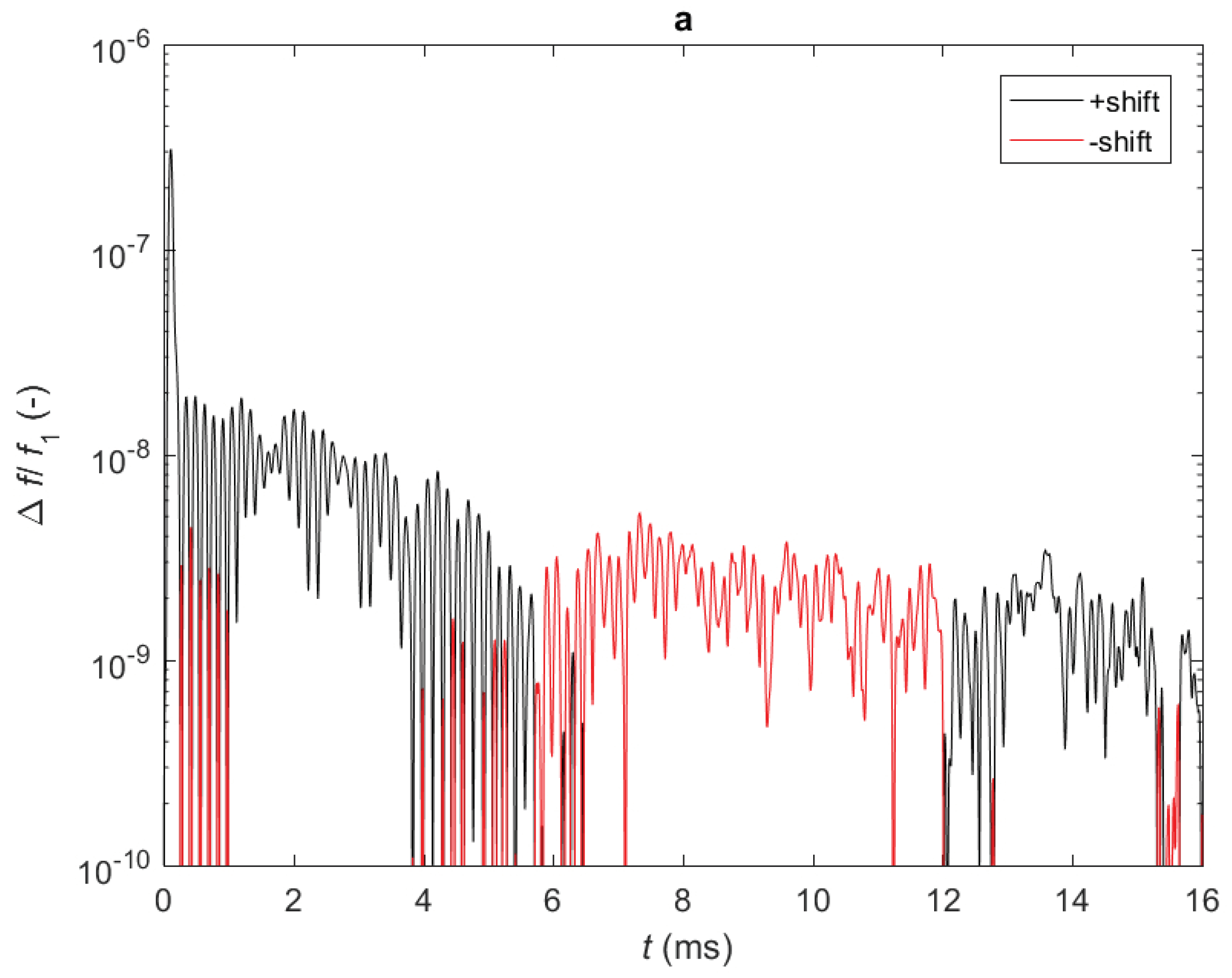
  The first approach requires a change in the collision frequency without a change in the electron density and the collision frequency of one of the states, which can be obtained by e.g., calculations based on cross-section data. As the expected changes in resonant behavior are only $\Delta f/f_1\sim -{10}^{-9}$ and $\Delta (1/Q)\sim {10}^{-10}$ (for ${\nu }_1$ = 50 GHz, ${\nu }_2$ = 1 THz, $n_{\mathrm{e},1}=n_{\mathrm{e},2}={10}^9$ m${}^{-3}$ and $f_{\mathrm{res}}$ = 3.5 GHz), it will require a high sensitivity in the measurement approach;

  -

  In the second approach, no restrictions to changes in the electron dynamics are required. The collision frequencies and electron densities need to be determined which requires the usage of at least two resonant modes or another diagnostic method to determine the collision frequencies.

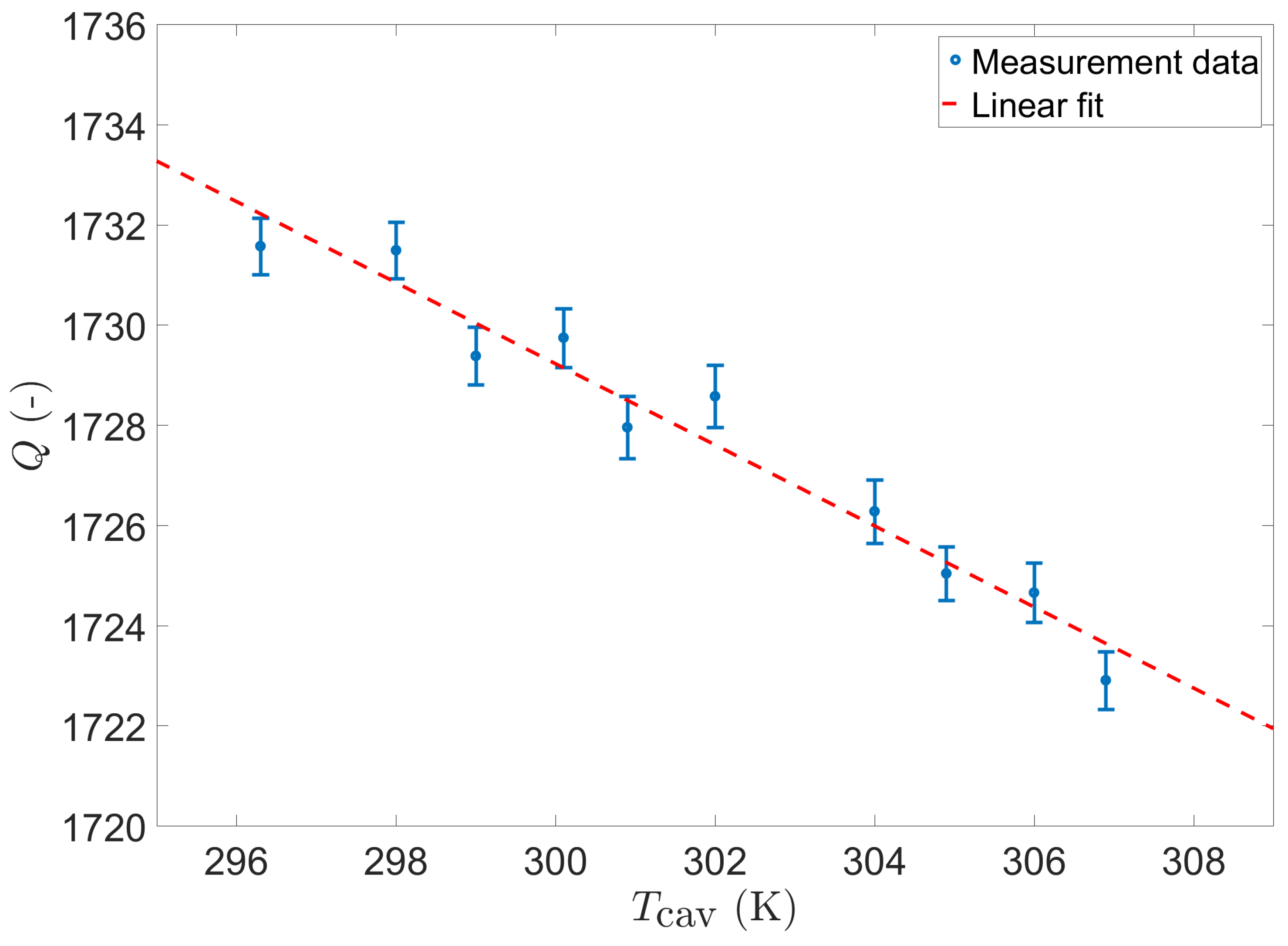
  The polarizability of the medium depends on its temperature [17] and this complicates the execution of the proposed experiments. Other factors which need to be taken into account are the expansion of the cavity volume and the change in conductance of the walls due to temperature variations.

Some general advice and ideas for (potential) users of the MCRS method are listed below.

• As MCRS is sensitive to almost everything, it is crucial to separate the different contributions to the detected change in resonant behavior. A step forward would be to perform MCRS measurements using multiple cavities in parallel in one solid block of metal. An example of this approach would be one cavity—preferably in vacuum conditions—could be used to monitor the conductivity and the dimensions of the metal structure surrounding the cavity, another without a discharge to compensate for the properties of the gas and a third to monitor the discharge;
• Section 3.5.2 demonstrated that not all higher-order modes are sensitive enough—when the plasma is placed at a node—to probe the electron dynamics of an atmospheric-pressure plasma jet. However, these could be used to study plasma-produced acoustic waves. This is another approach to separate contributions to changes in resonant behavior;
• The measurement time or the number of cavities can be reduced by applying multiple frequencies simultaneously in one cavity and separating the responses by an electronic filter;
• Resonant modes with the same cut-off frequency are referred to as degenerate modes. The usage of these type of modes can be cumbersome because the microwave field in a cavity tends to alternate over time between these modes. Furthermore, the fitting becomes more complex when resonance peaks (almost) overlap. For these reasons, degenerate modes should be avoided or all but one excluded in the design of a cavity;
• Integrating the antenna with (a part of) the cavity walls would result in a smaller perturbation from the ideal resonant field. Hence, this would result in more accurate usage of calculated electromagnetic field profiles;
• Manufacturing a stable cavity proved to be difficult. Vacuum soldering of the parts to create a metal structure—which forms the cavity—from one solid metal block showed the best approach. This approach with a solid cavity and correcting the response for temperature fluctuations is completely contradictory to the inventions in which the response of the cavity is temperature-stabilized by moving parts [63,64,65,66];
• The accuracy in determining the quality factor is lower than that of the resonance frequency. For this reason, it might be beneficial to use the change in the resonance frequency of multiple modes to separate the contributions of the electron density and the collision frequency to changes in resonant behavior. This approach requires the cavity to be filled homogenously with plasma and large differences between the resonance frequencies of the modes. Other methods to measure Q [2] potentially provide a higher resolution than the approach used in our prior works.

Some practical advice with a strong focus on the experimental setup and method used in references [18,19,20].

• The current approach—with frequency-resolved measurements—requires many reproducible discharges. A more direct scheme with good temporal resolution would be a huge step forward. Examples of approaches that require less complicated analysis, although with a poor temporal resolution, are described in the following articles [7,41,67].
• In all MCRS experiments performed by the authors, an equidistant frequency domain is used. The spectral positions of the probing frequencies can be optimized by allowing non-equidistant positions between two subsequent positions in the frequency domain. This will reduce the measurement time or increase the resolution in permittivity;
• Commercial network analyzers provide a calibration procedure to compensate for non-ideal properties of the load. The setup used here does not have such a function and therefore undesired oscillations are present in the spectral response. An example of a spectrum with these oscillations can be seen in Figure 2 of reference [18]. These undesired features increase the error in the results and can be troublesome for the user. Users would benefit from similar functionality as available in network analyzers;
• In the experiments performed by the authors, only cylindrical cavities were used. Cuboid cavities do not suffer from rotation of the resonant field of higher-order azimuthal modes due to e.g., perturbations by the plasma and could help to increase the accuracy of the results;
• Tuning of the antenna in a cavity is a very important step to obtain good results. Positioning the antenna with a micrometre screw gauge would be a good improvement to the current design of the cavities.

5. Conclusions

In this review article, a manifesto is presented for probing collisional plasmas with Microwave Cavity Resonance Spectroscopy. The discussed topics might be able to help to further develop the diagnostic method and explain unexpected results. The main messages of this article can be summarized as follows:

• The resolution in the resonant behavior—and therefore in the permittivity—is improved by several advancements in the measurement approach. Based on an experimental study, the dependency of this resolution on the number of averages and the size of the frequency sweep step is explained and translated to the optimal parameters with respect to the needed measurement time and resolution. Additionally, the influence of the quality factor on the resolution is explained;
• As smaller changes in the resonant behavior can be resolved due to recent improvements of the method, the electron dynamics are no longer the only contributor to changes in the permittivity during plasma experiments. The improvements to the diagnostic method enabled measuring—non-selectively—a new range of physical properties, e.g., gas composition, gas pressure, and the number density of metastables, etc. For this reason, we recommend thinking of permittivity as the main parameter when analyzing MCRS measurements rather than $n_{\mathrm{e}}$ and ${\nu }_{\mathrm{m}}$. Furthermore, a more detailed description is given of the temperature-corrected apparent frequencies that have been introduced in [19];
• For plasmas where the collision frequency of the electrons could not be neglected with respect to the applied angular microwave frequencies and also have a spatial dependency, the interpretation of the measurement data and the obtained $n_{\mathrm{e}}$ requires special care. The determination of the collision frequency of the electrons in a plasma with a spatial profile is very susceptible to errors of multiple orders of magnitude;
• In the two MCRS studies of atmospheric-pressure discharges [18,19], a camera was used to determine the volume which is occupied by the plasma. This volume together with the calculated resonant field profile is used to estimate the effective volume ratio $\mathcal{V}$. The uncertainty in the volume occupied by the plasma, and subsequently in $\mathcal{V}$, limits the accuracy of the determination of the electron density to its order of magnitude [18]. A set of improvements concerning this topic is proposed;
• The linearity of the shift in resonance frequency with the change of permittivity—or more traditionally the electron density—is investigated for a wide range of plasma parameters such as geometric dimensions, electron-neutral collision frequencies, and electron densities. Moreover, the correlation between the radius and the position of the plasma column with the mode structure is explored in relation to the lower limit of the permittivity or in archaic terms the upper limit of the electron density. In all investigated conditions, the putative limit ${\omega }_{\mathrm{pe}}$ ≪ $\omega$ was too stringent;
• Penetration of the microwaves into the plasma is crucial for successful MCRS measurements. For this reason, the skin depth is investigated for a variety of plasma parameters. Moreover, the calculated skin depths are compared with the results obtained in the previous section. This comparison showed that the limit $r_{\mathrm{p}}\ll \delta$ is in some cases to pessimistic in limiting the operational regime of MCRS.

Although there are still significant challenges for users of the diagnostic method, the advancements of the last few years have brought many new opportunities.

References

1. Biondi, M.A.; Brown, S.C. Measurements of ambipolar diffusion in helium. Phys. Rev. 1949, 75, 1700. [Google Scholar] [CrossRef]
2. Brown, S.C.; Rose, D.J. Methods of measuring the properties of ionized gases at high frequencies. I. Measurements of Q. J. Appl. Phys. 1952, 23, 711–718. [Google Scholar] [CrossRef] [Green Version]
3. Rose, D.J.; Brown, S.C. Methods of measuring the properties of ionized gases at high frequencies. II. Measurement of electric field. J. Appl. Phys. 1952, 23, 719–722. [Google Scholar] [CrossRef]
4. Rose, D.J.; Brown, S.C. Methods of measuring the properties of ionized gases at high frequencies. III. Measurement of discharge admittance and electron density. J. Appl. Phys. 1952, 23, 1028–1032. [Google Scholar] [CrossRef]
5. Gould, L.; Brown, S.C. Methods of measuring the properties of ionized gases at high frequencies. IV. A null method of measuring the discharge admittance. J. Appl. Phys. 1953, 24, 1053–1056. [Google Scholar] [CrossRef]
6. Franek, J.; Nogami, S.; Koepke, M.; Demidov, V.; Barnat, E.V. A Computationally Assisted Ar I Emission Line Ratio Technique to Infer Electron Energy Distribution and Determine Other Plasma Parameters in Pulsed Low-Temperature Plasma. Plasma 2019, 2, 65–76. [Google Scholar] [CrossRef] [Green Version]
7. Faltýnek, J.; Kudrle, V.; Tesar, J.; Volfová, M.; Tálský, A. Numerical enhancements of the microwave resonant cavity method for plasma diagnostics. Plasma Sources Sci. Technol. 2019, 28, 105007. [Google Scholar] [CrossRef]
8. Beckers, J.; Stoffels, W.W.; Kroesen, G.M.W. Temperature dependence of nucleation and growth of nanoparticles in low pressure Ar/CH4 RF discharges. J. Phys. D: Appl. Phys. 2009, 42. [Google Scholar] [CrossRef]
9. Wattieaux, G.; Carrasco, N.; Henault, M.; Boufendi, L.; Cernogora, G. Transient phenomena during dust formation in a N2-CH4 capacitively coupled plasma. Plasma Sources Sci. Technol. 2015, 24. [Google Scholar] [CrossRef]
10. Alcouffe, G.; Cavarroc, M.; Cernogora, G.; Ouni, F.; Jolly, A.; Boufendi, L.; Szopa, C. Capacitively coupled plasma used to simulate Titan’s atmospheric chemistry. Plasma Sources Sci. Technol. 2010, 19. [Google Scholar] [CrossRef]
11. Stoffels, E.; Stoffels, W.W.; Vender, D.; Kando, M.; Kroesen, G.M.W.; De Hoog, F.J. Negative ions in a radio-frequency oxygen plasma. Phys. Rev. E 1995, 51, 2425–2435. [Google Scholar] [CrossRef] [PubMed]
12. Van Ninhuijs, M.A.W.; Daamen, K.A.; Franssen, J.G.H.; Conway, J.; Platier, B.; Beckers, J.; Luiten, O.J. Microwave cavity resonance spectroscopy of ultracold plasmas. Phys. Rev. A 2019, 100, 061801. [Google Scholar] [CrossRef]
13. Van Der Horst, R.M.; Beckers, J.; Nijdam, S.; Kroesen, G.M.W. Exploring the temporally resolved electron density evolution in extreme ultra-violet induced plasmas. J. Phys. D Appl. Phys. 2014, 47, 7–11. [Google Scholar] [CrossRef] [Green Version]
14. Beckers, J.; Van De Wetering, F.M.J.H.; Platier, B.; Van Ninhuijs, M.A.W.; Brussaard, G.J.H.; Banine, V.Y.; Luiten, O.J. Mapping electron dynamics in highly transient EUV photon-induced plasmas: A novel diagnostic approach using multi-mode microwave cavity resonance spectroscopy. J. Phys. D Appl. Phys. 2019, 52, 034004. [Google Scholar] [CrossRef] [Green Version]
15. Platier, B.; Limpens, R.; Lassise, A.C.; Staps, T.J.A.; van Ninhuijs, M.A.W.; Daamen, K.A.; Luiten, O.J.; IJzerman, W.L.; Beckers, J. Transition from ambipolar to free diffusion in an EUV-induced argon plasma. Appl. Phys. Lett. 2020, 116, 103703. [Google Scholar] [CrossRef] [Green Version]
16. Birnbaum, G.; Kryder, S.J.; Lyons, H. Microwave measurements of the dielectric properties of gases. J. Appl. Phys. 1951, 22, 95–102. [Google Scholar] [CrossRef]
17. Magnuson, D.W. Microwave Dielectric Constant Measurements. J. Chem. Phys. 1956, 24, 344–347. [Google Scholar] [CrossRef]
18. Van Der Schans, M.; Platier, B.; Koelman, P.M.J.; Van De Wetering, F.M.J.H.; Van Dijk, J.; Beckers, J.; Nijdam, S.; IJzerman, W.L. Decay of the electron density and the electron collision frequency between successive discharges of a pulsed plasma jet in N2. Plasma Sources Sci. Technol. 2019, 28, 035020. [Google Scholar] [CrossRef]
19. Platier, B.; Staps, T.J.A.; Van Der Schans, M.; IJzerman, W.L.; Beckers, J. Resonant microwaves probing the spatial afterglow of an RF plasma jet. Appl. Phys. Lett. 2019, 115, 254103. [Google Scholar] [CrossRef] [Green Version]
20. Platier, B.; Staps, T.J.A.; Hak, C.C.J.M.; Beckers, J.; IJzerman, W.L. Resonant microwaves probing acoustic waves from an RF plasma jet. Plasma Sources Sci. Technol. 2020, 29, 045024. [Google Scholar] [CrossRef]
21. Persson, K.B. Limitations of the Microwave Cavity Method of Measuring Electron Densities in a Plasma. Phys. Rev. 1957, 106, 191–195. [Google Scholar] [CrossRef]
22. Agdur, B.; Enander, B. Resonances of a microwave cavity partially filled with a plasma. J. Appl. Phys. 1962, 33, 575–581. [Google Scholar] [CrossRef]
23. Buchsbaum, S.J.; Brown, S.C. Microwave measurements of high electron densities. Phys. Rev. 1957, 106, 196–199. [Google Scholar] [CrossRef]
24. Pleasance, L.D.; George, E.V. Electron density in ion-laser discharges. Appl. Phys. Lett. 1971, 18, 557–561. [Google Scholar] [CrossRef]
25. Sadeghi, N. Comment on: Correlating metastable-atom density, reduced electric field, and electron energy distribution in the post-transient stage of a 1 Torr argon discharge (2015 Plasma Source Sci. Technol. 24 034009). Plasma Sources Sci. Technol. 2016, 25. [Google Scholar] [CrossRef] [Green Version]
26. Van De Wetering, F.M.J.H. Formation and Dynamics of Nanoparticles in Plasmas. Ph.D. Thesis, Eindhoven University of Technology, Eindhoven, The Netherlands, 2016. [Google Scholar]
27. Shohet, J.L.; Hatch, A. Eigenvalues of a microwave cavity filled with a plasma of variable radial density. J. Appl. Phys. 1970, 41, 2610–2618. [Google Scholar] [CrossRef]
28. Souw, E.K. Plasma density measurement in an imperfect microwave cavity. J. Appl. Phys. 1987, 61, 1761–1772. [Google Scholar] [CrossRef]
29. Guochang, X.; Jun, L. Perturbation theoretical analysis and its application for TM010-mode microwave cavity of a gas laser. Rev. Sci. Instruments 1997, 68, 1935–1938. [Google Scholar] [CrossRef]
30. Platier, B.; van de Wetering, F.M.J.H.; van Ninhuijs, M.; Brussaard, S.; Banine, V.Y.; Luiten, O.J.; Beckers, J. Addendum: Mapping electron dynamics in highly transient EUV photon-induced plasmas: A novel diagnostic approach using multi-mode microwave cavity resonance spectroscopy (2018 J PHYS D APPL PHYS 52 034004). J. Phys: D. Appl. Phys 2020. [Google Scholar] [CrossRef]
31. Van De Wetering, F.M.J.H.; Beckers, J.; Kroesen, G.M.W. Anion dynamics in the first 10 milliseconds of an argon–acetylene radio-frequency plasma. J. Phys. D: Appl. Phys. 2012, 45, 485205. [Google Scholar] [CrossRef] [Green Version]
32. Green, E.I. The Story of Q. Am. Sci. 1955, 434, 584–594. [Google Scholar]
33. Harrington, R.F. Time-Harmonic Electromagnetic Fields; Wiley-IEEE Press: New York, NY, USA, 2001. [Google Scholar]
34. Lieberman, M.A.; Lichtenberg, A.J. Discharges and Materials Processing Principles of Plasma Discharges and Materials, 2nd ed.; Wiley Online Library: Hoboken, NJ, USA, 2005. [Google Scholar]
35. Chen, L.F.; Ong, C.K.; Neo, C.P.; Varadan, V.V.; Varadan, V.K. Measurement and Materials Characterization; John Wiley & Sons: West Sussex, UK, 2004; pp. 37–42. [Google Scholar] [CrossRef]
36. Raizer, J.P.; Shneider, M.N.; Yatsenko, N.A. Radio-Frequency Capacitive Discharges, 1st ed.; CRC Press: Boca Raton, FL, USA, 1995. [Google Scholar]
37. Bruggeman, P.J.; Iza, F.; Brandenburg, R. Foundations of atmospheric pressure non-equilibrium plasmas. Plasma Sources Sci. Technol. 2017, 26. [Google Scholar] [CrossRef] [Green Version]
38. Knappmiller, S.; Robertson, S.; Sternovsky, Z. Comparison of two microwave and two probe methods for measuring plasma density. IEEE Trans. Plasma Sci. 2006, 34, 786–791. [Google Scholar] [CrossRef] [Green Version]
39. Van De Wetering, F.M.J.H.; Brooimans, R.J.C.; Nijdam, S.; Beckers, J.; Kroesen, G.M.W. Fast and interrupted expansion in cyclic void growth in dusty plasma. J. Phys. D Appl. Phys. 2015, 48, 35204. [Google Scholar] [CrossRef] [Green Version]
40. Beckers, J.; Van Der Horst, R.M.; Osorio, E.A.; Kroesen, G.M.; Banine, V.Y. Thermalization of electrons in decaying extreme ultraviolet photons induced low pressure argon plasma. Plasma Sources Sci. Technol. 2016, 25. [Google Scholar] [CrossRef]
41. Freiberg, R.J.; Weaver, L.A. Microwave investigation of the transition from ambipolar to free diffusion in afterglow plasmas. Phys. Rev. 1968, 170, 336–341. [Google Scholar] [CrossRef]
42. Gerber, R.A.; Gerardo, J.B. Ambipolar-to-free diffusion: The temporal behavior of the electrons and ions. Phys. Rev. A 1973, 7, 781–790. [Google Scholar] [CrossRef]
43. Haverlag, M.; Kroesen, G.M.W.; Bisschops, T.H.J.; De Hoog, F.J. Measurement of electron densities by a microwave cavity method in 13.56-MHz RF plasmas of Ar, CF4, C2F6, and CHF3. Plasma Chem. Plasma Process. 1991, 11, 357–370. [Google Scholar] [CrossRef]
44. Stoffels, W.W.; Sorokin, M.; Remy, J. Charge and charging of nanoparticles in a SiH4 rf-plasma. Faraday Discuss. 2007, 137, 115–126. [Google Scholar] [CrossRef] [PubMed]
45. Van Der Horst, R.M.; Beckers, J.; Osorio, E.A.; Banine, V.Y. Exploring the electron density in plasmas induced by extreme ultraviolet radiation in argon. J. Phys. D Appl. Phys. 2015, 48. [Google Scholar] [CrossRef] [Green Version]
46. Leski, J.M. Robust weighted averaging [of biomedical signals]. IEEE Trans. Biomed. Eng. 2002, 49, 796–804. [Google Scholar] [CrossRef] [PubMed]
47. Agdur, N.B. Apparatus for Measuring the Properties of a Material by Resonance Techniques. US Patent 3,458,808, 29 July 1969. [Google Scholar]
48. Nelson, S.O.; Trabelsi, S. Factors influencing the dielectric properties of agricultural and food products. J. Microw. Power Electromagn. Energy 2012, 46, 93–107. [Google Scholar] [CrossRef] [PubMed]
49. Platier, B.; Limpens, R.; Lassise, A.C.; Oosterholt, T.T.J.; van Ninhuijs, M.A.W.; Daamen, K.A.; Staps, T.J.A.; Zangrando, M.; Luiten, O.J.; IJzerman, W.L.; et al. Magnetic field-enhanced beam monitor for ionizing radiation. Rev. Sci. Instruments 2020, 91, 063503. [Google Scholar] [CrossRef]
50. Haynes, W. CRC Handbook of Chemistry and Physics, 92th ed.; CRC Press: Boca Raton, FL, USA, 2011; pp. 6–209. [Google Scholar]
51. Pozar, D.M. Microwave Engineering, 4th ed.; John Wiley & Sons: Hoboken, NJ, USA, 2011. [Google Scholar]
52. Szewczyk, R. Magnetostatic Modelling of Thin Layers Using the Method of Moments and Its Implementation in Octave/Matlab; Lecture Notes in Electrical Engineering, Springer International Publishing: Cham, Switzerland, 2018; Volume 491. [Google Scholar] [CrossRef]
53. Anderson, J.M. Cavity method suitable for measurement of high electron densities in plasmas. Rev. Sci. Instruments 1961, 32, 975–978. [Google Scholar] [CrossRef]
54. Jackson, J.D.; Fox, R.F. Classical Electrodynamics. Am. J. Phys. 1999, 67, 841–842. [Google Scholar] [CrossRef]
55. Li, J.; Getmanov, I.K.; Kudryavtsev, A.A.; Yuan, C.; Wang, X.; Zhou, Z. Conductivity and Permittivity in Plasma with Nonequilibrium Electron Distribution Function. IEEE Trans. Plasma Sci. 2020, 48, 388–393. [Google Scholar] [CrossRef]
56. Schupp, R.; Torretti, F.; Meijer, R.A.; Bayraktar, M.; Scheers, J.; Kurilovich, D.; Bayerle, A.; Eikema, K.S.E.; Witte, S.; Ubachs, W.; et al. Efficient Generation of Extreme Ultraviolet Light from Nd:YAG-Driven Microdroplet-Tin Plasma. Phys. Rev. Appl. 2019, 12, 1. [Google Scholar] [CrossRef] [Green Version]
57. Ayvazyan, V.; Baboi, N.; Bähr, J.; Balandin, V.; Beutner, B.; Brandt, A.; Bohnet, I.; Bolzmann, A.; Brinkmann, R.; Brovko, O.I.; et al. First operation of a free-electron laser generating GW power radiation at 32 nm wavelength. Eur. Phys. J. D 2006, 37, 297–303. [Google Scholar] [CrossRef]
58. Zangrando, M.; Cudin, I.; Fava, C.; Gerusina, S.; Gobessi, R.; Godnig, R.; Rumiz, L.; Svetina, C.; Parmigiani, F.; Cocco, D. First results from the commissioning of the FERMI@Elettra free electron laser by means of the Photon Analysis Delivery and Reduction System (PADReS). In Advances in X-ray Free-Electron Lasers: Radiation Schemes, X-ray Optics, and Instrumentation; SPIE: Bellingham, WA, USA, 2011; Volume 8078, p. 80780I. [Google Scholar] [CrossRef]
59. Schreiber, S.; Faatz, B. The free-electron laser FLASH. High Power Laser Sci. Eng. 2015, 3. [Google Scholar] [CrossRef] [Green Version]
60. Milne, C.J.; Schietinger, T.; Aiba, M.; Alarcon, A.; Alex, J.; Anghel, A.; Arsov, V.; Beard, C.; Beaud, P.; Bettoni, S.; et al. SwissFEL: The Swiss X-ray Free Electron Laser. Appl. Sci. (Switzerland) 2017, 7, 720. [Google Scholar] [CrossRef]
61. Van Minderhout, B.; van Huijstee, J.; Platier, B.; Peijnenburg, T.; Blom, P.; Kroesen, G.M.W.; Beckers, J. Charge control of micro-particles in a shielded plasma afterglow. Plasma Sources Sci. Technol. 2020. [Google Scholar] [CrossRef]
62. Nijdam, S.; Takahashi, E.; Markosyan, A.H.; Ebert, U. Investigation of positive streamers by double-pulse experiments, effects of repetition rate and gas mixture. Plasma Sources Sci. Technol. 2014, 23. [Google Scholar] [CrossRef] [Green Version]
63. Niessen, K.F. Clamped Cavity Resonator. U.S. Patent 2,528,387, 31 October 1950. [Google Scholar]
64. Mccoubrey, M.O. Temperature Compensated Microwave Cavity. US Patent 3,034,078, 8 May 1962. [Google Scholar]
65. Atia, A.E.; Perimutter, D.; Schrantz, P.R. Temperature Compensation Apparatus for a Resonant Microwave Cavity. US Patent 4,156,860, 29 May 1979. [Google Scholar]
66. Pome, E.; Giovanni, S.S. Temperature Stabilied and Frequency Adjustable Microwave Cavities. US Patent 4,335,365, 15 June 1982. [Google Scholar]
67. Franek, J.B.; Nogami, S.H.; Demidov, V.I.; Koepke, M.E.; Barnat, E.V. Correlating metastable-atom density, reduced electric field, and electron energy distribution in the post-transient stage of a 1-Torr argon discharge. Plasma Sources Sci. Technol. 2015, 24. [Google Scholar] [CrossRef] [Green Version]
68. Chew, W.C. Lectures on Theory of Microwave and Optical Waveguides. 2012. Available online: http://wcchew.ece.illinois.edu/chew/course/tgwAll20121211.pdf (accessed on 12 October 2019).
69. Feynman, R.P. Feynman Lectures on Physics: V2; Naroga Publishing House: New Delhi, India, 2013. [Google Scholar]
Figure 1. The amplitude of the electric field | E | of the fundamental resonant mode (TM 010 ) in a cylindrical resonant cavity.
Applsci 10 04331 g001
Figure 2. Spectral response of the TM 010 resonant mode of the unperturbed cavity measured in reflection configuration (red marks) and a Lorentzian fit (blue line).
Applsci 10 04331 g002
Figure 3. The change in the (a) real and (b) imaginary part of the relative permittivity of a plasma as a function of the electron density for four collision frequencies. The imaginary part of the permittivity is zero when the electrons do not collide and for this reason there is no change in the imaginary part of the permittivity for ν m = 0 Hz.
Applsci 10 04331 g003aApplsci 10 04331 g003b
Figure 4. A schematic representation of the experimental setup comprising the plasma source, the resonance cavity, and the control and read-out electronics. B. Platier, T. J. A. Staps, M. van der Schans, W. L. IJzerman, and J. Beckers, Applied Physics Letters, Vol. 115, Article ID 254103, 2019; licensed under a Creative Commons Attribution (CC BY) license.
Applsci 10 04331 g004
Figure 5. Temporal evolution of (a) the relative frequency shift Δ f / f 1 , (b) the change of the reciprocal quality factor Δ ( 1 / Q ) , (c) the electron density n e , and (d) the effective electron collision frequency ν eff for different plasma repetition frequencies f rep . The Roman numerals (I, II, III, and IV) indicate the four distinctive plasma phases in the experiment. B. Platier, T. J. A. Staps, M. van der Schans, W. L. IJzerman, and J. Beckers, Applied Physics Letters, Vol. 115, Article ID 254103, 2019; licensed under a Creative Commons Attribution (CC BY) license.
Applsci 10 04331 g005
Figure 6. The electric field magnitude of the TM 010 mode inside and in the vicinity of the cavity. B. Platier, T. J. A. Staps, M. van der Schans, W. L. IJzerman, and J. Beckers, Applied Physics Letters, Vol. 115, Article ID 254103, 2019; licensed under a Creative Commons Attribution (CC BY) license.
Applsci 10 04331 g006
Figure 7. (a) Temporal evolution of the relative frequency shift Δ f / f 1 where the negative values are indicated in red and the positive shifts in black. (b) The pressure difference Δ p for air (green) and He (magenta) required to induce a shift in the resonance frequency as presented in (a) are shown. The cyan line indicates the data for He after a second moving average processing step. B. Platier, T. J. A. Staps, C. C. J. M. Hak, J. Beckers, and W. L. IJzerman, Plasma Sources Science and Technology, https://doi.org/10.1088/1361-6595/ab7d8e, 2020; licensed under a Creative Commons Attribution (CC BY) license.
Applsci 10 04331 g007aApplsci 10 04331 g007b
Figure 8. The evolution of the pressure difference caused by acoustic waves. The dashed lines are there to guide the eye. B. Platier, T. J. A. Staps, C. C. J. M. Hak, J. Beckers, and W. L. IJzerman, Plasma Sources Science and Technology, https://doi.org/10.1088/1361-6595/ab7d8e, 2020; licensed under a Creative Commons Attribution (CC BY) license.
Applsci 10 04331 g008
Figure 9. The coefficient of variation, i.e., the normalized standard deviation of Δ ( 1 / Q ) (red) and Δ f (blue) as a function of the number of averages (square) and the frequency step size (circle). The results indicated by triangular symbols show the effect of averaging 20 consecutive time steps.
Applsci 10 04331 g009
Figure 10. The exponent β which indicates the noise reduction in Δ ( 1 / Q ) (red) and Δ f (blue) as a function of the number of averages (square) and the frequency step size (circle) with respect to the reference measurement with 4096 averages and a frequency step size of 1 kHz. The results indicated by triangular symbols show the effect of averaging 20 consecutive time steps. The theoretically expected β is indicated by the horizontal dashed line.
Applsci 10 04331 g010
Figure 11. The quality factor Q as a function of the temperature of the metal structure surrounding the cavity T cav . The circles represent the measurement data and the dashed line is obtained by a linear fit procedure using the experimental data.
Applsci 10 04331 g011
Figure 12. The ratio between the plasma parameters, i.e., (a) the collision frequency of the electrons and (b) the electron density, obtained by the measurement approach used for collisional plasmas and the electric-field-squared-weighted averaged values as a function of the collision frequency in region 2 ν m , 2 for several n e , 2 .
Applsci 10 04331 g012
Figure 13. The coaxial geometry where the outer cylinder is the volume occupied by the resonance cavity and the inner cylinder is an homogenous plasma column.
Applsci 10 04331 g013
Figure 14. Investigation of the linearity of the relative resonance frequency shift Δ f f 1 as a function of the change of the relative permittivity Δ ε r of the TM 010 and TM 110 mode for four plasma radii. The vertical dashed line at Δ ε r = 1 indicates the expanded putative limit of the Microwave Cavity Resonance Spectroscopy (MCRS) diagnostic method and the circles indicate where the response is no longer linear.
Applsci 10 04331 g014aApplsci 10 04331 g014b
Figure 15. Investigation of the linearity of the relative resonance frequency shift Δ f f 1 as a function of the change of the relative permittivity Δ ε r of the plasma ( r p = 10 4 m) for eight resonant modes. The vertical dashed line at Δ ε r = 1 indicates the expanded putative limit of the MCRS diagnostic method and the circles indicate where the response is no longer linear.
Applsci 10 04331 g015aApplsci 10 04331 g015b
Figure 16. The skin depth of a plasma for three collision frequencies as a function of the change in permittivity Δ ε ˜ with respect to ε 0 . Furthermore, the parameters in which the shift of the resonance frequency no longer scales linearly with a change in permittivity are indicated by circles for a variety of modes—red circles for plasma at an antinode and black circles for at a node—and plasma radii.
Applsci 10 04331 g016