Structural Damage Features Extracted by Convolutional Neural Networks from Mode Shapes

Abstract

This paper aims to locate damaged rods in a three-dimensional (3D) steel truss and reveals some internal working mechanisms of the convolutional neural network (CNN), which is based on the first-order modal parameters and CNN. The CNN training samples (including a large number of damage scenarios) are created by ABAQUS and PYTHON scripts. The mode shapes and mode curvature differences are taken as the inputs of the CNN training samples, respectively, and the damage locating accuracy of the CNN is investigated. Finally, the features extracted from each convolutional layer of the CNN are checked to reveal some internal working mechanisms of the CNN and explain the specific meanings of some features. The results show that the CNN-based damage detection method using mode shapes as the inputs has a higher locating accuracy for all damage degrees, while the method using mode curvature differences as the inputs has a lower accuracy for the targets with a low damage degree; however, with the increase of the target damage degree, it gradually achieves the same good locating accuracy as mode shapes. The features extracted from each convolutional layer show that the CNN can obtain the difference between the sample to be classified and the average of training samples in shallow layers, and then amplify the difference in the subsequent convolutional layer, which is similar to a power function, finally it produces a distinguishable peak signal at the damage location. Then a damage locating method is derived from the feature extraction of the CNN. All of these results indicate that the CNN using first-order modal parameters not only has a powerful damage location ability, but also opens up a new way to extract damage features from the measurement data.

1. Introduction

Structural damage detection, as an important part of structural health monitoring (SHM), aims to timely and accurately find out structural problems so that corresponding maintenances can be taken to ensure the safety and reliability of a structure during its service period. At present, the commonly used damage detection methods include appearance inspection, sample surveys, ultrasonic wave and X-ray, which are used to detect local internal and external defects of structures [1]; there are also other methods like static test methods, which are used to obtain static parameters of structures, such as structural stiffness, deflection, strain and moment of inertia. These detecting methods not only need a large amount of manpower and material resources, but also require a high professional skills and vast engineering experience of detection, in addition to the long detecting cycle and subjective assessment [2]. Dynamic detection methods based on structural modal parameters become a research hotspot in recent decades and are gradually applied to engineering practice owing to its nondestructive, cost-effective, and efficient characteristics [3]. Meanwhile, the rapid development of digital measurement technology provides solid technical supports for the accurate measurement of structural dynamic responses. The applications of Digital Image Correlation (DIC) technology [4] and Unmanned Aerial Vehicles (UAVs) in damage detection [5,6] also make the structural dynamic measurement more convenient and simpler. As the modal parameters (modal frequencies and mode shapes) of a structure represent its state and its local damage will cause their changes, which can be used to identify the change of the structure state [7]. However, these modal parameters are not always sensitive to a small damage, which makes it difficult and inefficient to determine the damage location through these modal parameters. Therefore, more effective indexes are generated, such as mode shape curvature and modal strain energy, etc. [8,9,10,11,12], which are more sensitive to a small damage of a structure. However, the traditional damage detection methods often misjudge damages or miss a damage for large and complex structures. As a damage of a structure often causes the changes of multiple damage indexes, while the traditional structural damage detection methods are all based on a single damage index, which cannot completely describe all the damage features of a complex structure. Therefore, it is vital to find a powerful tool to extract the damage features of a complex structure. With their powerful data processing ability and good robustness, neural networks can extract the features of measured data, thus they can be used to explore the structural performances under different damage scenarios.

Over the last few decades, the back propagation (BP) neural network performed better in damage detection [13,14] among many artificial neural networks applied in damage detection. However, it is slow converging, time-consuming, and prone to over fitting [15]. Now, the convolutional neural network (CNN), which includes convolutional layers into the neural network, has better feature extraction ability and overcomes some drawbacks of the BP neural networks. In recent years, deep learning algorithms based on CNNs have shown their superior performance in the field of SHM, several papers have studied the SHM data anomaly detection [16], crack recognition [17], mass change [18], damage detection of a three-dimensional (3D) steel frame [19], and the first-order sensitivity-based method was used for matching the FE model and the real model [20]. As easily obtained modal parameters, the first-order mode shape can be used as the CNN inputs. Though, low-order mode shapes are usually less sensitive to structural damages, the CNN can extract damage features from low-order mode shapes, which are not distinguishable for naked eyes; its excellent ability of feature extraction could make up the disadvantages of low-order mode shapes. As low-order mode shapes are relatively easy to obtain, combining them with CNNs could greatly increase the effectiveness of structural damage detection. At present, there are few studies combining CNNs with low order mode shapes. On the other hand, although CNNs have been applied to structural damage detection by many studies owing to its good performance, it was only used as a powerful “black box”, its feature extraction mechanisms are to be explored, which will undoubtedly promote the further development of CNN methods.

In this paper, the first order mode shape is taken as the input of a CNN to study the CNN accuracy in locating the damaged rods of a 3D steel truss. At the same time, because the curvature difference of the first order mode shape has distinguishable peak features at the damaged segment, this paper also takes it as the CNN input to study its locating accuracy. As the CNN has been widely used in SHM as a powerful “black box”, it is necessary to have more in-depth understanding of its working mechanism, which is important for the further application of the CNN, as people can analyze whether the predicted results are accurate and identify the possible causes of errors, and even can obtain more damage information from measurement data through the CNN methods. To this end, this paper explores the basis of damage classification of the CNN by comparing the difference between the inputs and outputs of each convolutional layer. To use this powerful tool to find more structural damage indexes and the extraction methods to obtain these indexes, some internal working mechanisms of the CNN are studied.

2. Method

In this paper, the modal data of a steel truss with various damage scenarios are obtained through finite element simulations, they are used as the inputs of a CNN to train the network and investigate the prediction accuracy of the CNN. Meanwhile, the output of each convolutional layer is extracted to study the internal working mechanism of the CNN.

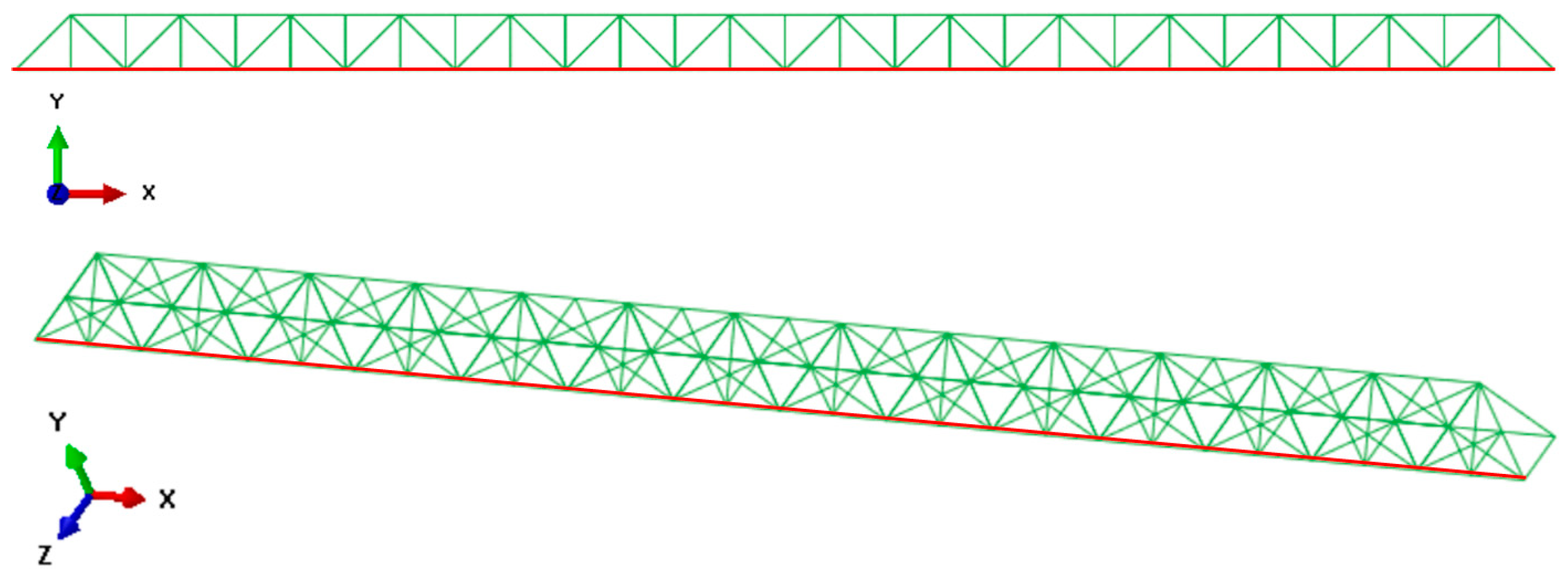
2.1. Finite Element Simulations

This paper uses a steel truss as the structural model (Figure 1); its length, width and height are 9.912 m, 0.354 m, and 0.354 m. Its left and right ends are simply supported. The truss consists of 355 rods; each rod has a hollow circular cross section with an external radius of 0.005 m and a thickness of 0.002 m. The Young’s modulus, Poisson’s ratio, density, and modal damping of the model are 211 GPa, 0.288, 7800, and 0.02 kg/m³, respectively.

The finite element software package, ABAQUS (SIMULIA Inc., Providence, RI, USA), is used to obtain the modal parameters of the steel truss, while PYTHON scripts are used to prepare the input files of the finite element analyses for a variety of designed damage scenarios and submit the analyses to ABAQUS solver. The first order mode shapes and the mode curvature differences are used respectively to train the CNN.

There are 16 damage degrees and 355 damage locations used in this study. The structural damage is defined as changes to the elastic modulus of the rod concerned. It is assumed that the damage degree of a rod has a linear relation with the reduction of its elastic modulus, so that this paper uses 16 damage degrees, the elastic modulus of which is respectively reduced by 0%, 2%, 4%, 5%, 6%, 8%, 10%, 20%, 30%, 40%, 50%, 60%, 70%, 80%, 90%, 95% from the intact state, while for each damage degree, there are 355 damage locations to represent the damage in each of the 355 rods respectively, hence, there are a total of 5326 damage scenarios.

This paper only considers single damage scenarios, i.e., each scenario has only one rod damaged.

2.2. Training Samples

The input data of the CNN training samples are derived from the vertical displacement of the rods on the front lower edge of the truss (the red line in Figure 1). There are 28 rods along this line; each rod has 8 observation points, the observation points at both ends of the adjacent rods coincide with each other, so there are a total of 197 observation points, the vertical displacement in the first order mode of which are obtained to form the mode shapes samples. The mode shape curvatures can be calculated by the following formula:

$${{\varphi }_k}^{\prime \prime }=\frac{{\varphi }_{k-1}-2{\varphi }_k+{\varphi }_{k+1}}{{\left(\mathsf{\Delta }l\right)}^2}$$

(1)

where ${\varphi }_k$ is the vertical displacement of the k-th point, and $\mathsf{\Delta }l=0.05\mathrm{m}$, it is the distance between two adjacent points. The mode curvature difference is the difference between the curvatures of a damage scenario and the intact scenario. Thus, each mode curvature difference sample contains 195 data. To ensure these two kinds of samples have the same dimension, the first and the last datum of the mode shape samples are removed. Therefore, each sample is a 1 × 195 row vector and is arranged into a 15 × 13 matrix. Since there are 16 damage degrees and 355 damage locations, there are 5326 samples for each index. The samples for damage degrees of 0%, 2%, 5%, 8%, 20%, 40%, 60%, 80%, and 95% were selected as the training set and the samples for damage degrees of 0%, 4%, 6%, 10%, 30%, 50%, 70%, and 90% were selected as the test set.

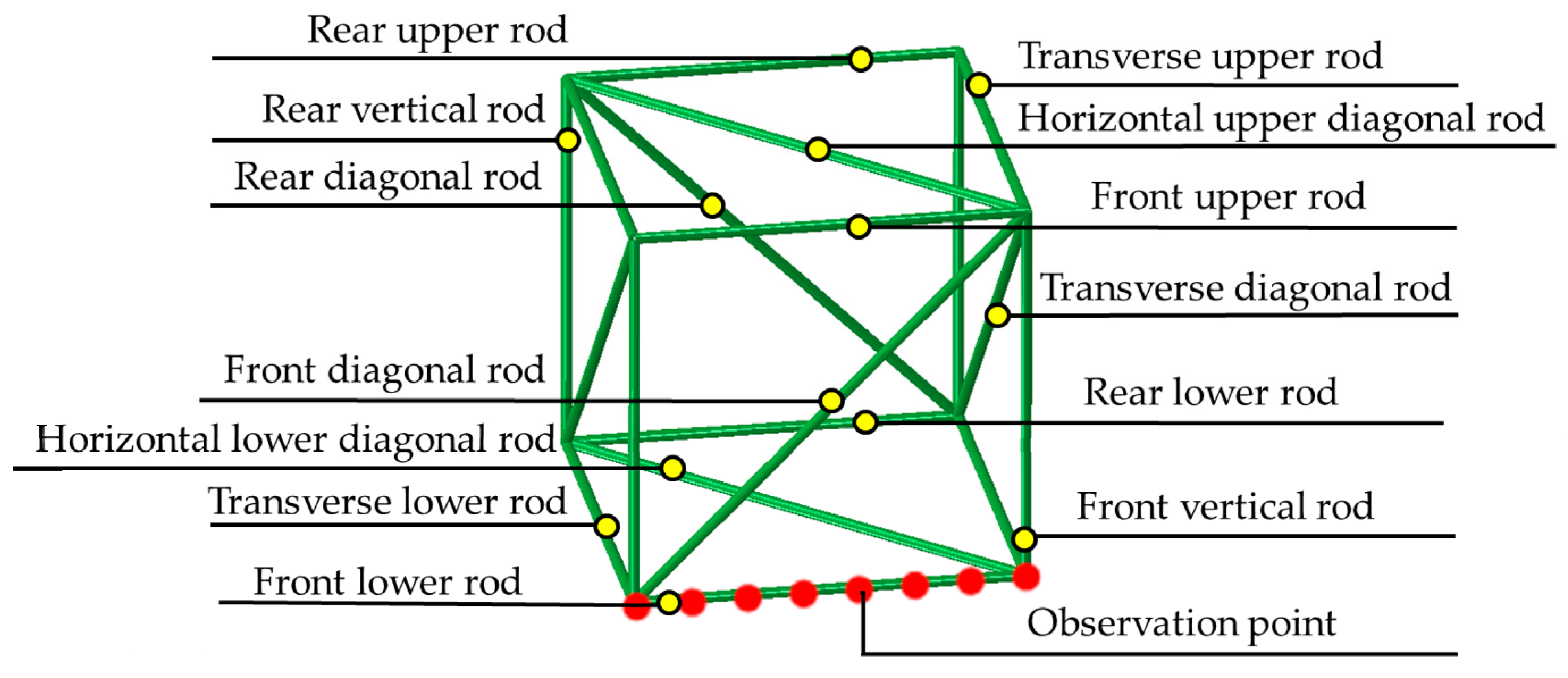
2.3. Structural Damage Detection

In this paper, the classification function of the CNN is used to locate damaged rods. As a different damage scenario will produce a different structural mode, therefore, the classification function of the CNN can be used to classify different damage scenario by matching the mode samples and damage scenarios one to one, so as to realize the detection of damage degree and location.

The CNN input is the modal parameters of different damage scenarios, while the CNN output is the label of different damage scenarios. That is, each damage scenario is marked with a label, starting with the damage of 2% in Rod 1 being marked as Label 1, then the damage of 2% in Rod 2 will be marked as Label 2, and so on. The label number increases consecutively for next damage degree, for example, the damage of 4% in Rod 1 will be marked as Label 356. In the end, the damage of 95% in Rod 355 is marked as Label 5325. Label 5326 is for the intact truss.

The whole training process is divided into training phase and testing phase. Firstly, the CNN conducts network training according to the one-to-one input and output relationship. The training is mainly to update the CNN weights and reduce the error between the actual outputs and the target outputs. When the training phase is completed, the trained network can be saved and the test samples are inputted to the network. By comparing the target outputs with the actual outputs of the network, the prediction accuracy of damage location can be obtained. Figure 2 is the seventh span of the steel truss, which shows the naming convention of the rods.

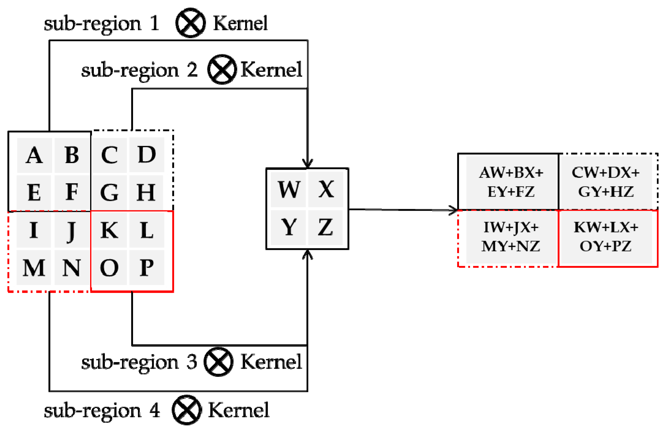
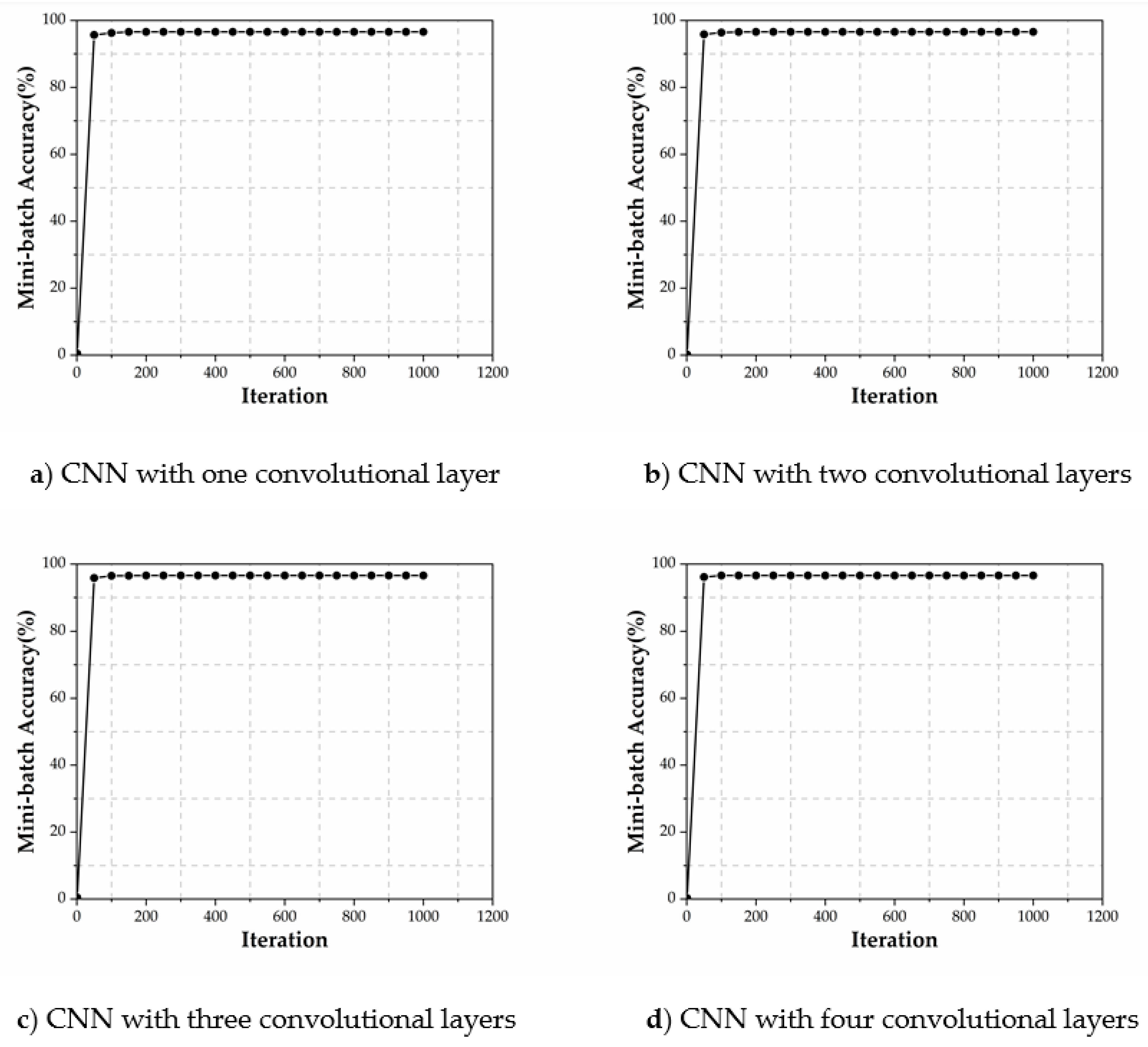
2.4. CNN Architecture

The architecture of the CNN (Figure 3) is designed in MATLAB (MathWorks Inc., Natick, MA, USA). It mainly includes an input layer, four convolutional layers, a fully-connected layer, a softmax layer and an output layer.

The convolution process is shown in Figure 4. A fixed-size convolution kernel is used to multiply the corresponding elements of each sub-region of the input matrix then sum them up to be an element in the new matrix. Then the convolution kernel slides with a fixed stride (the stride in Figure 4 is 2); the process is repeated until all elements of the input elements are involved; finally, it forms a new matrix and then it will be mapped nonlinearly by the activation function and normalized in the batch normalization layer.

After the input data passes through the four convolutional layers, it is fully expanded into a one-dimensional column vector by the flatten layer and then enters the fully-connected layer. The probability that a sample belongs to a target class is calculated by the softmax layer. The softmax is a function of the following form:

$$P\left(i\right)=\frac{\exp \left({\theta }_i^{T}x\right)}{{\displaystyle \sum _{k=1}^n\exp \left({\theta }_k^{T}x\right)}}$$

(2)

where $P\left(i\right)$ is the probability that a sample belongs to the i-th class, $x$ is the input in a column vector form, $n$ is the number of classes, and $\theta$ is the undetermined coefficients in a column vector form.

When the sample finally enters the class output layer, the sample will be classified into the category with the highest probability.

3. Results

3.1. First Order Mode Shape as CNN Input

Through many trial calculations, it is found that the damage locating accuracy becomes higher as the convolutional layer increases. Figure 5 shows the training process for the convolutional layers being 1, 2, 3 and 4, respectively. Finally, the network having four convolutional layers is used. The kernel size of each layer is 3 × 3, 2 × 2, 1 × 1 and 1 × 1, respectively and the stride is 1; no pooling layers are used.

As shown in Figure 5, the CNN reaches a high accuracy after 1000 iterations. As for the test sets of different damage scenarios, the prediction accuracies are shown in

Table 1. Prediction accuracies of the first order mode shapes.

Prediction Accuracies
Type		Damage Degree
	0%	4%	6%	10%	30%	50%	70%	90%
Front lower rod		100%	100%	100%	100%	100%	92%	89%
Front upper rod		100%	100%	100%	100%	100%	96%	92%
Front vertical rod		100%	92%	100%	100%	100%	100%	100%
Front diagonal rod		100%	100%	100%	100%	100%	100%	96%
Rear lower rod		100%	100%	100%	100%	100%	100%	96%
Rear upper rod		50%	46%	38%	42%	46%	42%	46%
Rear vertical rod		63%	77%	81%	96%	92%	92%	92%
Rear diagonal rod		92%	92%	100%	100%	100%	100%	100%
Transverse lower rod		58%	58%	44%	65%	48%	58%	34%
Horizontal upper diagonal rod		96%	92%	96%	100%	100%	100%	100%
Transverse upper rod		14%	25%	37%	63%	81%	77%	40%
Horizontal lower diagonal rod		84%	96%	80%	92%	96%	92%	100%
Transverse diagonal rod		66%	63%	55%	55%	51%	85%	74%
Overall	100%	79%	80%	79%	85%	85%	87%	81%

:

Table 1 shows that a damage scenario can be distinguished from the intact state by the CNN trained with the first order mode shape as the CNN input, the damage prediction accuracy reaches 79% in low damage degree (4%), and increases to the maximum value of 87% for the damage degree of 70%. As for the rods around the observation point, such as the front lower rods, the front upper rods, the front vertical rods and the front diagonal rods, the prediction accuracy can reach 100% when the damage degree is only 4%.

3.2. Mode Curvature Difference as CNN Input

Because the mode curvature difference is more distinguishable at the damage location than the mode shape, it is used as the CNN input and the locating accuracy is investigated.

Through many trial calculations, it is found that the increase of the convolutional layers has slight effect on the training results. Figure 6 shows the training process for the convolutional layers being 1, 2, 3, and 4, respectively, the stride is 1 and there are no pooling layers.

Finally, the CNN with only one convolutional layer is selected for damage detection and the convolution kernel size is 1 × 1. As shown in Figure 6, the network reached a high accuracy after 100 iterations. As for its test sets, the prediction accuracies are shown in

Table 2. Prediction accuracies of the mode curvature differences.

Prediction Accuracies
Type		Damage Degree
	0%	4%	6%	10%	30%	50%	70%	90%
Front lower rod		57%	100%	100%	100%	100%	92%	100%
Front upper rod		76%	96%	100%	100%	100%	100%	100%
Front vertical rod		18%	44%	55%	100%	100%	100%	100%
Front diagonal rod		57%	78%	89%	100%	100%	100%	100%
Rear lower rod		21%	17%	53%	92%	100%	100%	100%
Rear upper rod		38%	38%	38%	57%	92%	92%	92%
Rear vertical rod		66%	74%	74%	59%	81%	59%	44%
Rear diagonal rod		7%	25%	10%	78%	96%	100%	100%
Transverse lower rod		10%	13%	13%	37%	44%	55%	27%
Horizontal upper diagonal rod		32%	35%	50%	71%	89%	85%	100%
Transverse upper rod		18%	33%	48%	74%	92%	74%	18%
Horizontal lower diagonal rod		26%	26%	19%	65%	92%	84%	92%
Transverse diagonal rod		7%	22%	44%	48%	88%	100%	92%
Overall	0%	33%	46%	53%	75%	90%	87%	82%

:

Table 2 shows that, selecting the first order mode curvature difference as the CNN input is unable to correctly distinguish the intact and damage scenarios sometimes. Its damage prediction accuracy is only 33% in the low damage degree (4%), but the prediction accuracy increases with the increase of damage degree, the accuracy reaches the maximum value of 90% when the damage degree increases to 50%. For the rods around the observation points, such as the front lower rod, the front upper rod and the front diagonal rod, the damage prediction accuracy is also significantly higher than other rods.

3.3. Data Feature Visualization

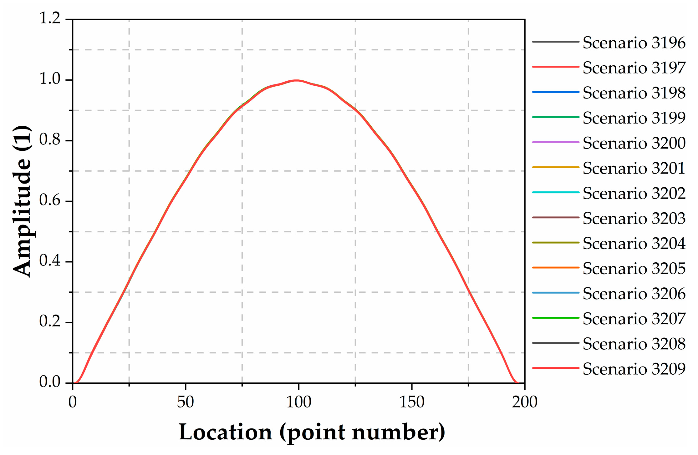
3.3.1. Sample Features

Some first order mode shape samples are shown in Figure 7. There are 14 curves of different damage scenarios in Figure 7 and these curves have different colors; but they are so similar that they look like only one curve. Some first order mode curvature difference samples are shown in Figure 8.

Figure 7 shows that, the first order mode shapes of various damage scenarios are almost the same, they are not distinguishable for naked eyes; on the other hand, the mode curvature differences show evident fluctuations in the damage locations (Figure 8).

As for the input data having distinguishable features, such as the mode curvature differences, the CNN can locate the damaged rods using the shallow learning rather than using the deep learning, as shown in Figure 6, the prediction accuracy is no longer improved when the layer number increases. While if the input data have no obvious fluctuations at the damage locations, such as the first order mode shapes, it requires deep learning to achieve a higher prediction accuracy, as shown in Figure 5, the prediction accuracy is gradually improved as the layer number increases.

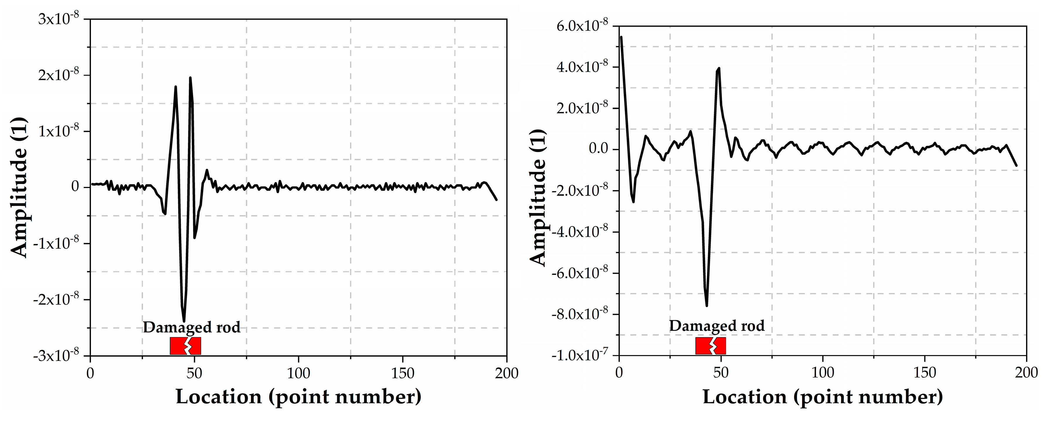
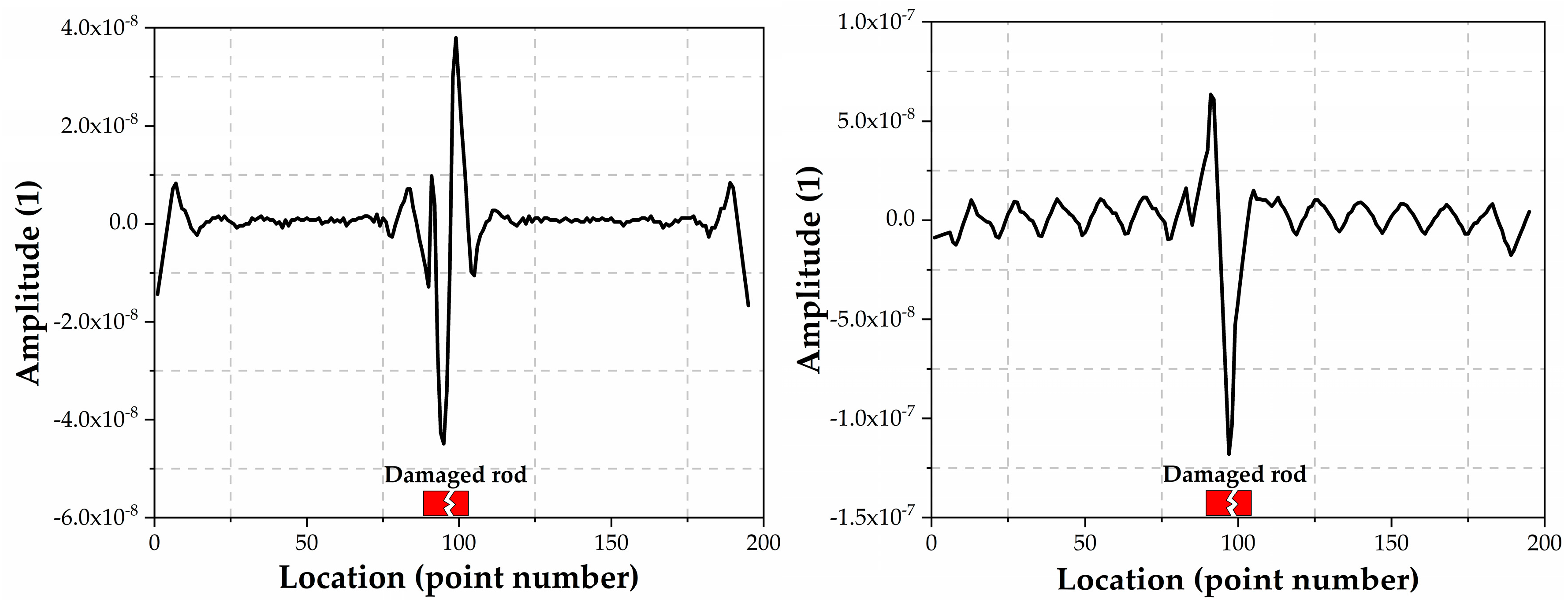
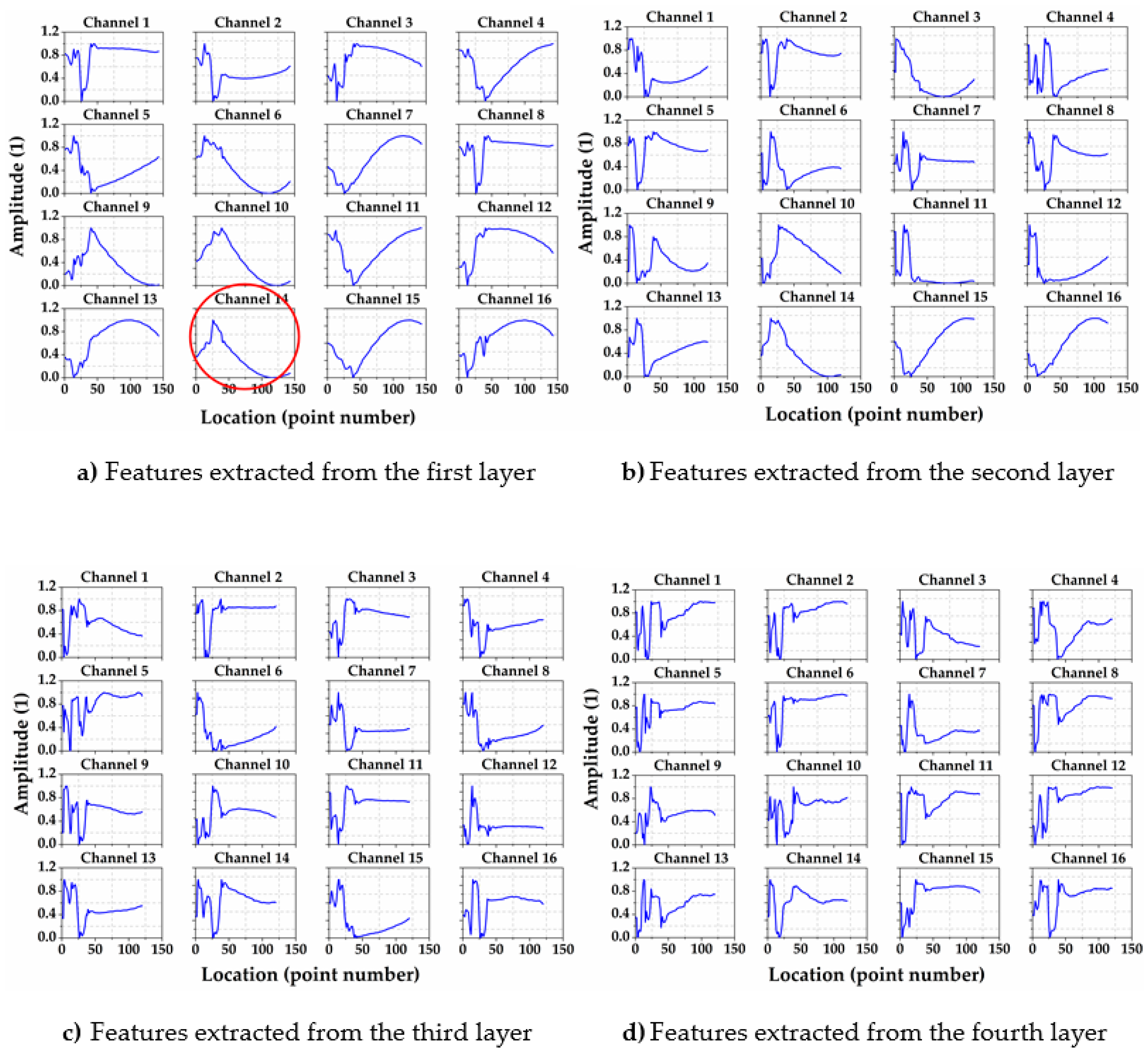
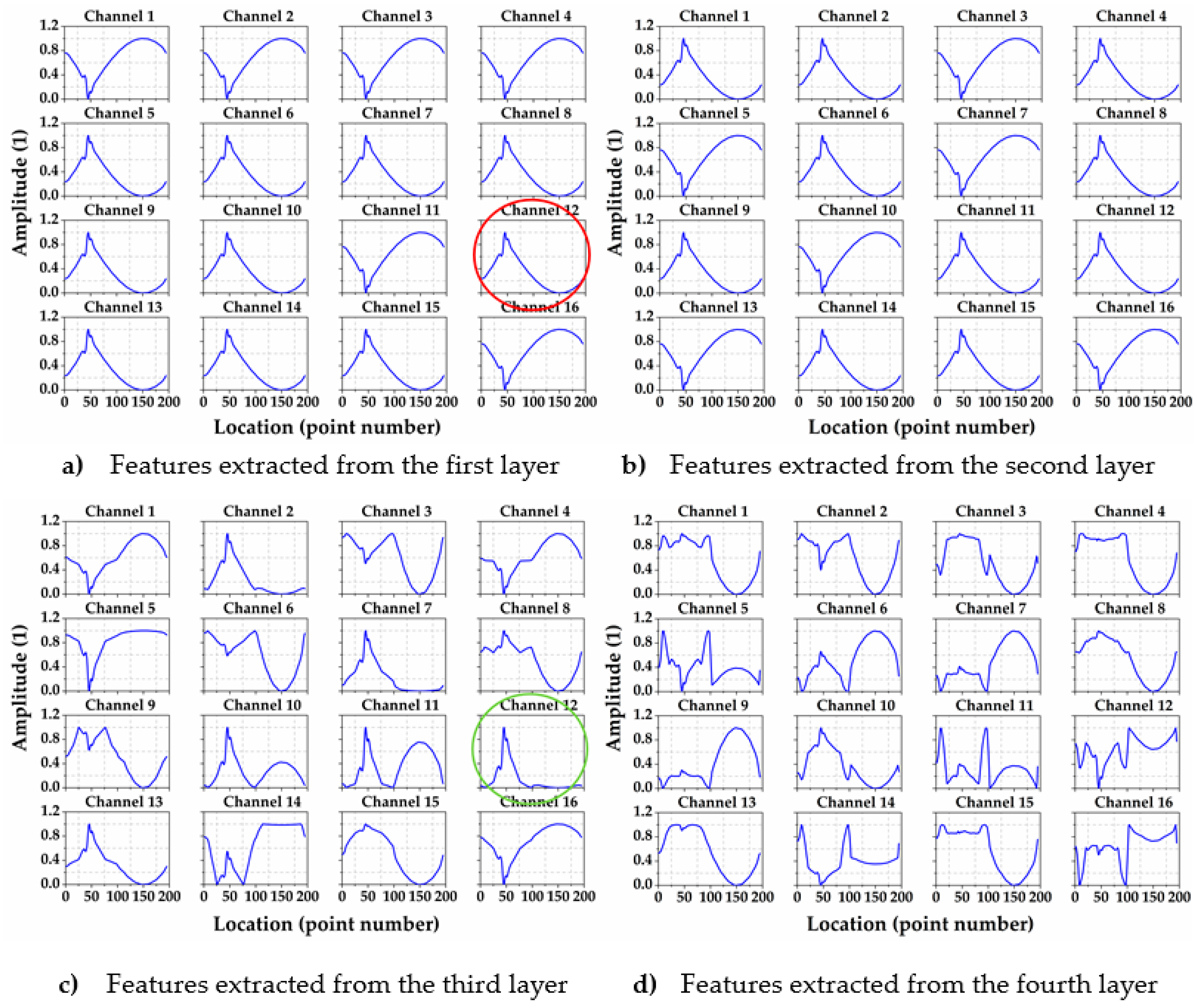
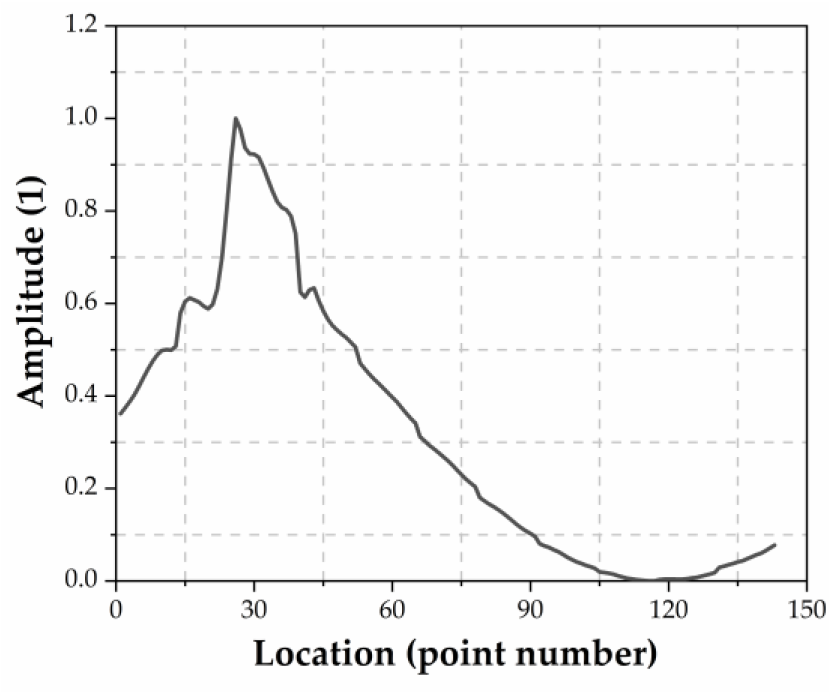
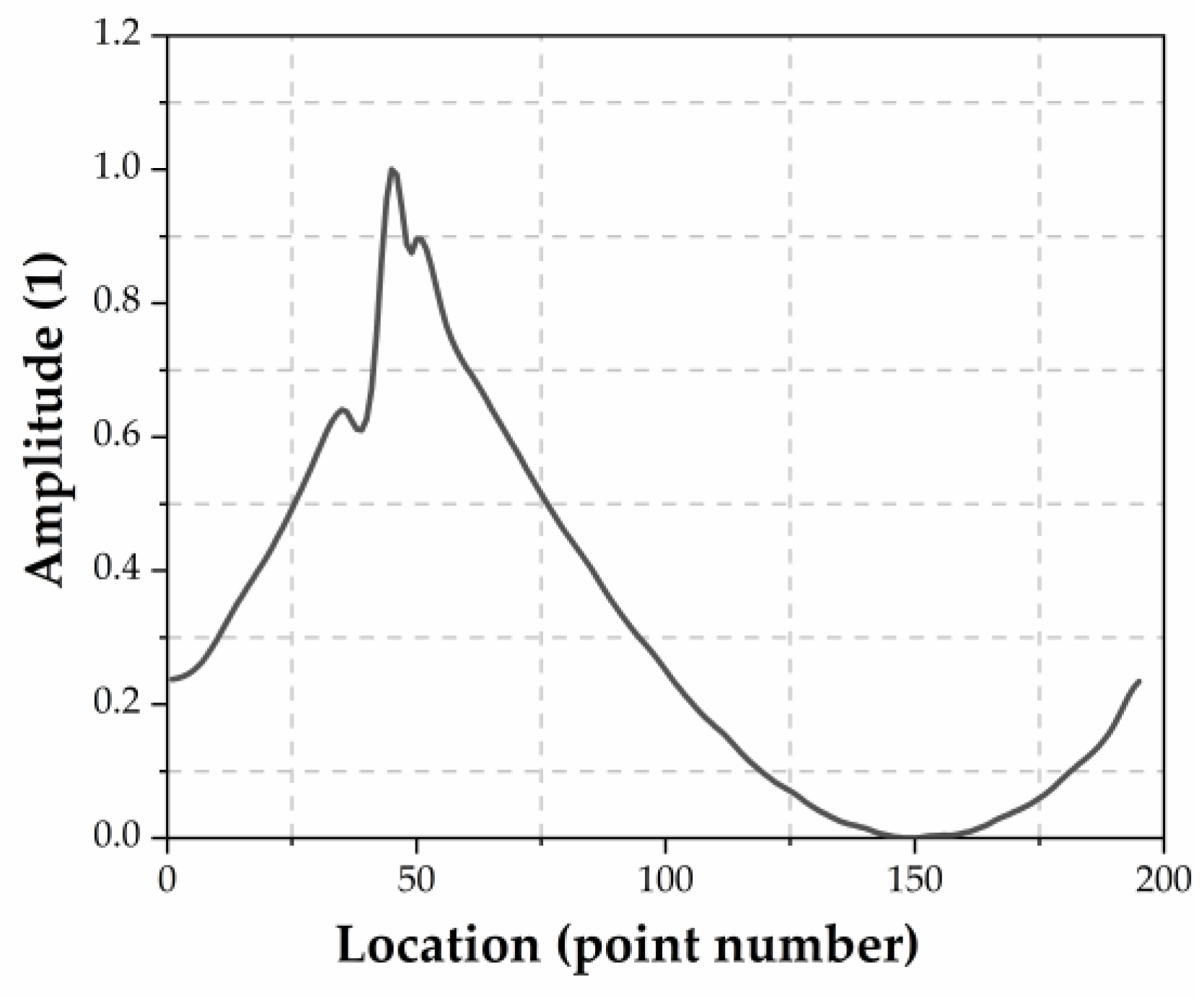
3.3.2. Features Extracted by the CNN

The function “activations” in the MATLAB Deep Learning Toolbox is used to get the features extracted by each convolutional layer. Figure 9 shows the output data of 16 channels of each layer, they represent the features extracted from the 3202-th damage scenario (the front lower rod in the seventh span with a damage of 50%) by the CNN. For all the curves, the x-coordinate is the location and the y-coordinate is its amplitude.

Because the convolution kernel size greater than 1 × 1 will decrease the data dimension, which makes the data difficult to compare, thus the kernels of the four convolutional layers are re-sized to 1 × 1 in the following context and the CNN is re-trained. The prediction accuracy reduced from 84% to 74% after changing the convolution kernel sizes. Figure 10 shows the features extracted from the 3202-th damage scenario by the CNN after the change of the convolution kernel size. As shown in Figure 9 and Figure 10, the features extracted by the two CNNs have certain similarity, especially in the shallow layers, for example, the features marked by red circles in Figure 9 and Figure 10 are very similar to each other. They are normalized and re-drawn in Figure 11 and Figure 12.

Firstly, try to explain the specific meaning of the feature extracted from the first convolutional layer (Figure 12). It is re-drawn on Figure 13 (Curve 1). At the same time, the difference between the average of the training samples and the sample of the 3202-th scenario is calculated and the normalized result is shown in Figure 13 (Curve 2), then the difference between the sample of intact scenario and the sample of the 3202-th scenario is calculated and the normalized result is shown in Figure 13 (Curve 3).

These figures show that the red-circled feature is very similar to the difference between the average of training samples and the sample of the 3202-th scenario, especially at the peak position, they almost overlap each other, but there are still some deviations in other position. The red-circled feature and the difference between the intact scenario and the 3202-th scenario show a better fitting, they almost overlap each other in all positions.

Secondly, the feature marked by green-circled in the third layer is considered. The normalized result is shown in Figure 14 (Curve 1), at the same time, the features extracted by the first convolutional layer (Figure 12) are mapped by a quadratic function and the result is shown in Figure 14 (Curve 2). The comparison shows that the two curves are almost identical, especially at the peak position.

The features in Figure 15 are extracted from the convolutional layers after the first order mode shape samples of other damage scenarios are inputted into the CNN. The features of the top row are extracted from the first convolutional layer for various damage scenarios and the features of the bottom row are from the third convolutional layer. All these features have the same performance as above, the first layer features are similar to the difference between the sample to be classified and the average of training samples, and the third layer features are similar to the mapping of the first layer features via a power function.

Through comprehensive observations of the features extracted from the first to the third layers, it can be found that the input samples produce distinguishable peak features at the damage location after three convolutional layers; the normalized result is very similar to the square of the difference between the sample to be classified and the average of training samples.

4. Discussions and Conclusions

This paper uses the CNN method to locate the damaged rod of a complex steel truss based on the first order mode shapes and mode curvature differences. It shows the prediction accuracies for a variety of damage scenarios and reveals some internal working mechanisms of the network.

Section 3.1. and Section 3.2 show that the CNN method based on the first order mode shape has a higher accuracy when locating the single damaged rod in all damage scenarios, even if the damage degree is only 4%, the prediction accuracies of some rods reach 100%, while the method based on the mode curvature difference can achieve the same prediction accuracy in locating the rod with a high damage degree, but the prediction accuracy is poor when locating the rod with a low damage degree. Section 3.3. shows the features of the two kinds of input data, compared with the first order mode shape (unprocessed data), the curvature difference (processed data) has obvious numerical variations at the damage location, but it does not have a better accuracy as expected, the central difference method may result in the loss of some information, while the original data like the first order mode shape may contain more damage information and the damage detection accuracy based on it is higher. Furthermore, to extract the inconspicuous features from the data, the CNN needs a deep learning architecture to get more powerful features extraction ability, hence, the CNN, using the first order mode shape as the inputs, needs a deep learning architecture to achieve higher accuracy; while the CNN, using the mode curvature difference as the inputs, only needs a shallow learning architecture to achieve its maximum prediction accuracy. However, even for the method based on the first order mode shape, there are always some rods with poor prediction accuracy. The reason may be that, only the vertical displacements of the truss are used as the inputs, they may not contain enough damage information.

By observing the features extracted from the mode shapes, it can be seen that the CNN can obtain the difference between the sample to be classified and the weighted average of the training samples in shallow layers, and then amplify the difference in the subsequent convolutional layer. Thus, it can be inferred that the partial work of the CNN to locate a damaged rod is to render the input data remarkable at the damage segment through updating the internal weights of the network, it appears like the result of calculating the difference between the sample to be classified and the weighted average of the training samples and then map it via a quadratic function. After the calculation of multiple convolutional layers, the mode shapes will have a distinguishable peak feature in the damaged segment like the curvature differences. This kind of data processing is very similar to the existing damage indexes based on the mode curvature differences, mode shape coefficient [21] and mode shape difference function [22], which were used traditionally to overcome the disadvantages of low-order mode shapes.

As the Figure 9 shows, there are certainly many other features extracted by the CNN, but their specific meanings are to be explored. The work above can only identify the damage existing in which segment; however, the CNN should be able to locate the damage existing in which rod. Besides, this paper ignored the function of the large size convolution kernel in the feature extractions; therefore, what the CNN does inside still needs a further exploration.

A neural network is a method simulating the biological neuron through mathematical algorithm model. Through the previous discussions, it can be found that it does something very similar to the human mind in the process of damage locating. By observing the features extracted by the CNN, a simple method of damage location can be derived, that is to calculate the difference between the sample to be classified and the sample of intact scenario to get the mode shape difference function and then map it via a power function to magnify the fluctuation feature, so as to produce a distinguishable peak in the damaged segment and finally locate the damaged segment. The formula is as follows:

$$f(x)={\varphi }^d(x)-\varphi (x)$$

(3)

$$f(x)={\varphi }^d(x)-\varphi (x)$$

(4)

$$F(x)={[f(x)]}^n$$

(5)

$f\left(x\right)$ = mode shape difference function

$\varphi$ = mode shape of the intact structure

${\varphi }^d$ = mode shape of the damaged structure

$x$ = spatial location

$n$ = power factor

From the above discussion, it can be concluded that:

• the CNN method based on the mode shape has a good prediction accuracy of damaged rods, but there are always some rods with low prediction accuracy. Due to the different sensitivity of modal data to the damage of different types of rods, their prediction accuracies are also different;
• the CNN method based on the mode curvature difference has similar good prediction accuracy to the mode shape when locating the rod with high damage degree. However, the prediction accuracy is low when locating the rods with small damage degree. Like the mode shape, there are always some rods with low prediction accuracy due to the different sensitivity of modal data to the damage of different rods;
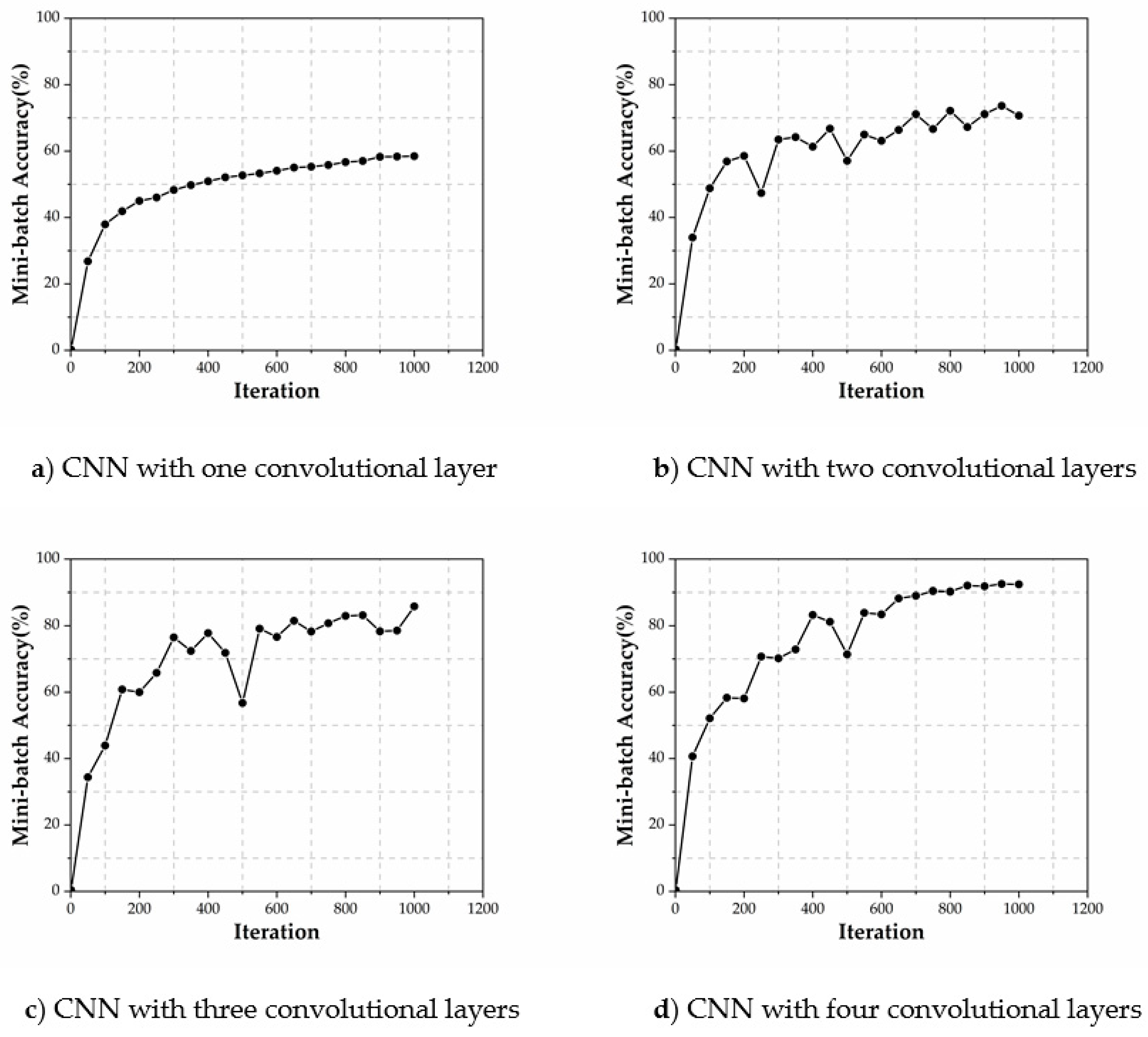
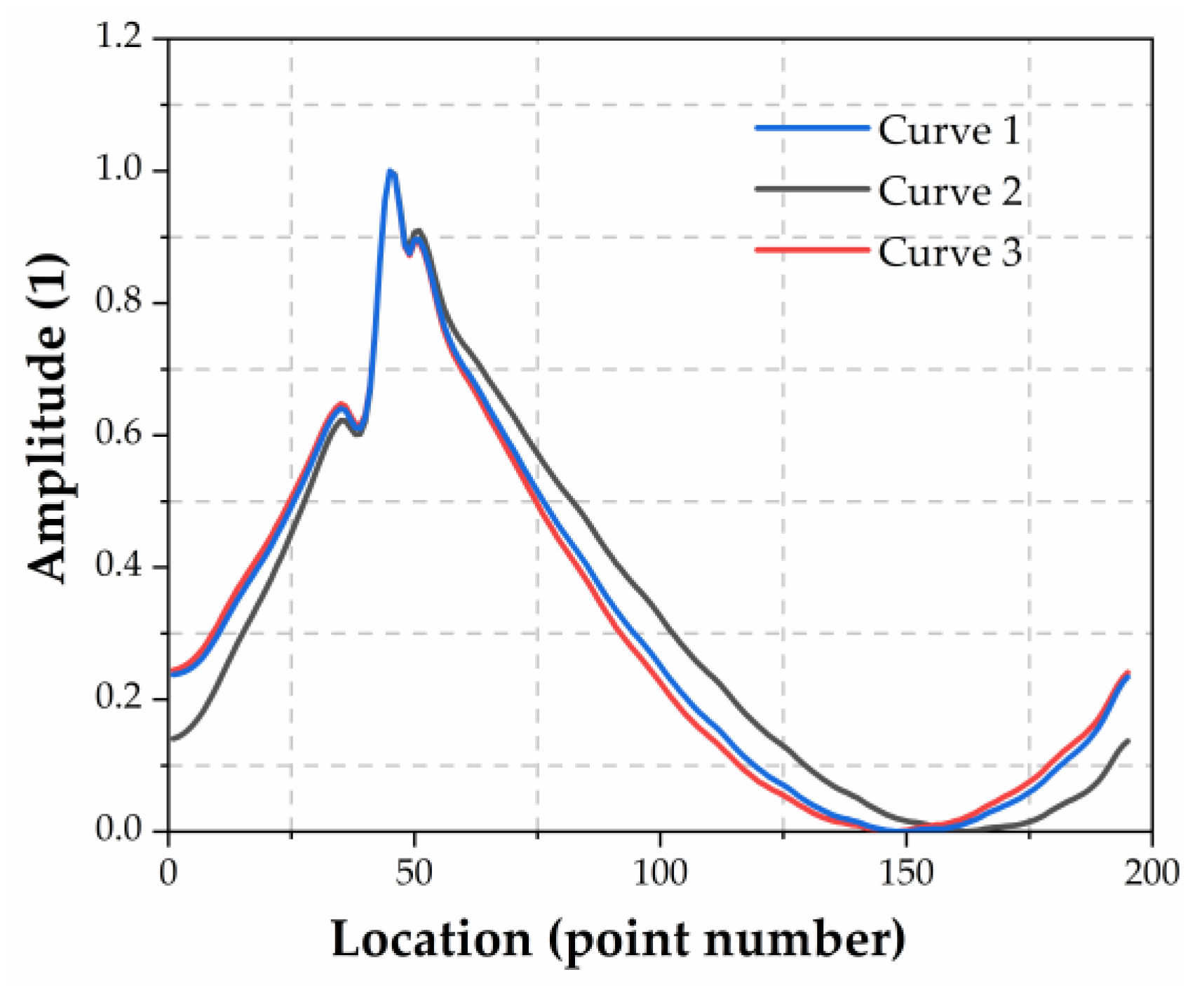
• the origin data has more damage information for the CNN. Though the first order mode shapes look indistinguishable, the multi-layer CNN can extract the damage information from the data, which are indistinguishable for naked eyes;
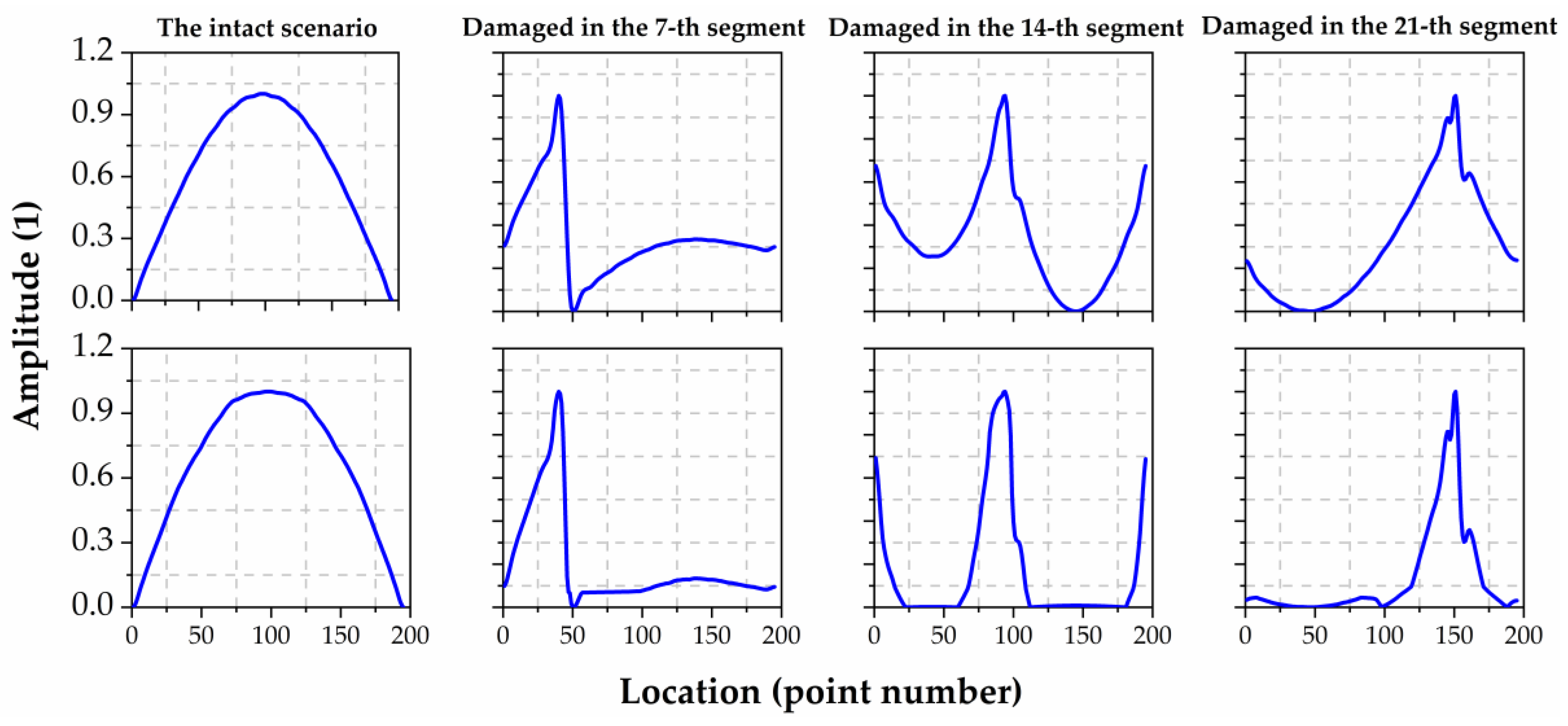
• using the first order mode shape as the input of the CNN to locate the damaged rod, the partial work of the CNN is to update its internal weights to get the difference between the input sample and the weighted average of the training samples in shallow layers, then the data will produce a distinguishable peak feature in the damaged segment after processed by multiple convolutional layers behind. This CNN process is similar to calculating the difference between the sample to be classified and the weighted average of the training samples and then mapping it via a quadratic function.

References

1. Ni, H.; Li, M.H.; Zuo, X. Review on Damage Identification and Diagnosis Research of Civil Engineering Structure. Adv. Mat. Res. 2014, 1006–1007, 34–37. [Google Scholar] [CrossRef]
2. Graybeal, B.A.; Phares, B.M.; Rolander, D.D.; Moore, M.; Washer, G. Visual Inspection of Highway Bridges. J. Nondestruct. Eval. 2002, 21, 67–83. [Google Scholar] [CrossRef]
3. Aguilar, R.; Zonno, G.; Lozano, G.; Boroschek, R.; Lourenço, P.B. Vibration-Based Damage Detection in Historical Adobe Structures: Laboratory and Field Applications. Int. J. Archit. Herit. 2019, 13, 1005–1028. [Google Scholar] [CrossRef]
4. Molina-Viedma, A.J.; Felipe-Ses, E.L.; López-Alba, E.; Díaz, F.A. Full-field modal analysis during base motion excitation using high speed 3D digital image correlation. Meas. Sci. Technol. 2017, 28. [Google Scholar] [CrossRef] [Green Version]
5. Lee, J.H.; Yoon, S.S.; Kim, I.H.; Jung, H.J. Diagnosis of crack damage on structures based on image processing techniques and R-CNN using unmanned aerial vehicle (UAV). In Proceedings of the SPIE Smart Structures and Materials + Nondestructive Evaluation and Health Monitoring, Sensors and Smart Structures Technologies for Civil, Mechanical, and Aerospace Systems, Denver, CO, USA, 27 March 2018; p. 1059811. [Google Scholar] [CrossRef]
6. Xiong, C.; Li, Q.; Lu, X. Automated regional seismic damage assessment of buildings using an unmanned aerial vehicle and a convolutional neural network. Autom. Constr. 2020, 109. [Google Scholar] [CrossRef]
7. Cawley, P.; Adams, R.D. The Location of defects in structures from measurements of natural frequencies. J. Strain Anal. Eng. Des. 1979, 14. [Google Scholar] [CrossRef]
8. Sundermeyer, J.N.; Weaver, R.L. On crack identification and characterization in a beam by non-linear vibration analysis. J. Sound Vib. 1995, 183, 857–871. [Google Scholar] [CrossRef]
9. Shi, Z.Y.; Law, S.S.; Zhang, L.M. Structural damage localization from modal strain energy change. J. Sound Vib. 1998, 218, 825–844. [Google Scholar] [CrossRef]
10. Zou, Y.; Tong, L.; Steven, G.P. Vibration-based model-dependent damage (delamination) and health monitoring for composite structures—a review. J. Sound Vib. 2000, 230, 357–378. [Google Scholar] [CrossRef]
11. Palacz, M.; Krawczuk, M. Vibration parameters for damage detection in structures. J. Sound Vib. 2002, 249, 999–1010. [Google Scholar] [CrossRef]
12. Xu, Z.D.; Wu, Z. Energy damage detection strategy based on acceleration responses for long-span bridge structures. Eng. Struct. 2006, 29, 609–617. [Google Scholar] [CrossRef]
13. Wu, X.; Ghaboussi, J.; Garrett, J.H. Use of neural networks in detection of structural damage. Comput. Struct. 1992, 42, 649–659. [Google Scholar] [CrossRef]
14. Zang, C.; Imregun, M. Structural Damage Detection Using Artificial Neural Networks and Measured Frf Data Reduced via Principal Component Projection. J. Sound Vib. 2001, 242, 813–827. [Google Scholar] [CrossRef]
15. Yao, W. The Researching Overview of Evolutionary Neural Networks. Comput. Sci. 2004, 31, 125–129. [Google Scholar] [CrossRef]
16. Tang, Z.; Chen, Z.; Bao, Y.; Li, H. Convolutional neural network-based data anomaly detection method using multiple information for structural health monitoring. Struct. Control. Health Monit. 2018, 26, e2296. [Google Scholar] [CrossRef] [Green Version]
17. Modarres, C.; Astorga, N.; Droguett, E.L.; Meruane, V. Convolutional neural networks for automated damage recognition and damage type identification. Struct. Control. Health Monit. 2018, 25, e2230. [Google Scholar] [CrossRef]
18. Zhang, Y.; Miyamori, Y.; Mikami, S.; Saito, T. Vibration-based structural state identification by a 1-dimensional convolutional neural network. Comput.-Aided Civ. Infrastruct. Eng. 2019, 34, 1–18. [Google Scholar] [CrossRef]
19. Teng, S.; Chen, G.; Gong, P.; Liu, G.; Cui, F. Structural damage detection using convolutional neural networks combining strain energy and dynamic response. Meccanica 2019, 0, 1–15. [Google Scholar] [CrossRef]
20. Teng, S.; Chen, G.; Liu, G.; Lv, J.; Cui, F. Modal Strain Energy-Based Structural Damage Detection Using Convolutional Neural Networks. Appl. Sci. 2019, 9, 3376. [Google Scholar] [CrossRef] [Green Version]
21. Frans, R.; Arfiadi, Y.; Parung, H. Comparative Study of Mode Shapes Curvature and Damage Locating Vector Methods for Damage Detection of Structures. Procedia Eng. 2017, 171, 1263–1271. [Google Scholar] [CrossRef]
22. Poudel, U.P.; Fu, G.; Ye, J. Wavelet transformation of mode shape difference function for structural damage location identification. Earthq. Eng. Struct. Dyn. 2007, 36, 1089–1107. [Google Scholar] [CrossRef]
Figure 1. Steel truss model.
Applsci 10 04247 g001
Figure 2. Naming convention of rods.
Applsci 10 04247 g002
Figure 3. Convolutional neural network (CNN) architecture.
Applsci 10 04247 g003
Figure 4. Convolution process.
Applsci 10 04247 g004
Figure 5. Training processes.
Applsci 10 04247 g005
Figure 6. Training processes.
Applsci 10 04247 g006
Figure 7. The first order mode shapes of various damage scenarios.
Applsci 10 04247 g007
Figure 8. Mode curvature differences of various damage scenarios.
Applsci 10 04247 g008aApplsci 10 04247 g008b
Figure 9. Features extracted from the 3202-th damage scenario by the CNN before the change of the convolution kernel size.
Applsci 10 04247 g009
Figure 10. Features extracted from the 3202-th damage scenario by the CNN after the change of the convolution kernel size.
Applsci 10 04247 g010
Figure 11. Feature extracted from the first convolutional layer before the change of the convolution kernel size.
Applsci 10 04247 g011
Figure 12. Feature extracted from the first convolutional layer after the change of the convolution kernel size.
Applsci 10 04247 g012
Figure 13. Comparisons of three curves. (a) Curve 1 is the feature extracted from the first convolutional layer (Figure 12); (b) Curve 2 is the difference between the average of training samples and the sample of the 3202-thscenario; (c) Curve 3 is the difference between the intact scenario and the 3202-th scenario.
Applsci 10 04247 g013
Figure 14. Comparisons of two curves. (a) Curve 1 is the feature extracted from the third layer; (b) Curve 2 is the square of the feature extracted from the first layer.
Applsci 10 04247 g014
Figure 15. The features of various damage scenarios extracted from the first (top row) and the third (bottom row) layers.
Applsci 10 04247 g015