Structural Damage Detection Based on Real-Time Vibration Signal and Convolutional Neural Network


Abstract
1. Introduction
2. Methods
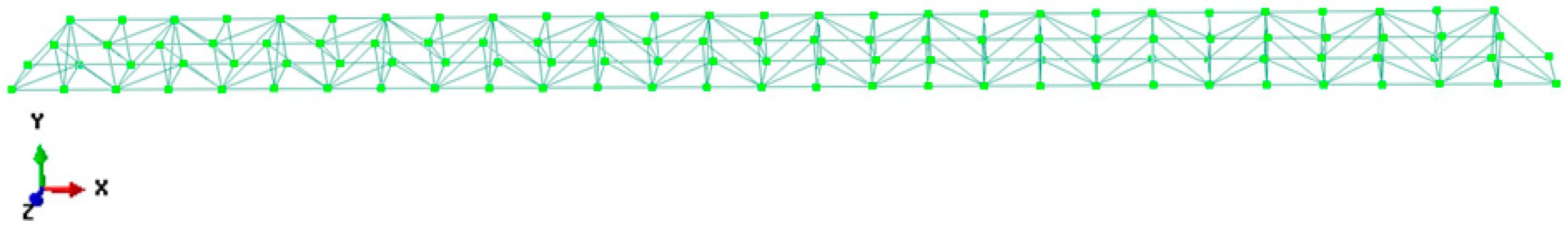
2.1. Numerical Simulations
2.2. Vibration Experiments
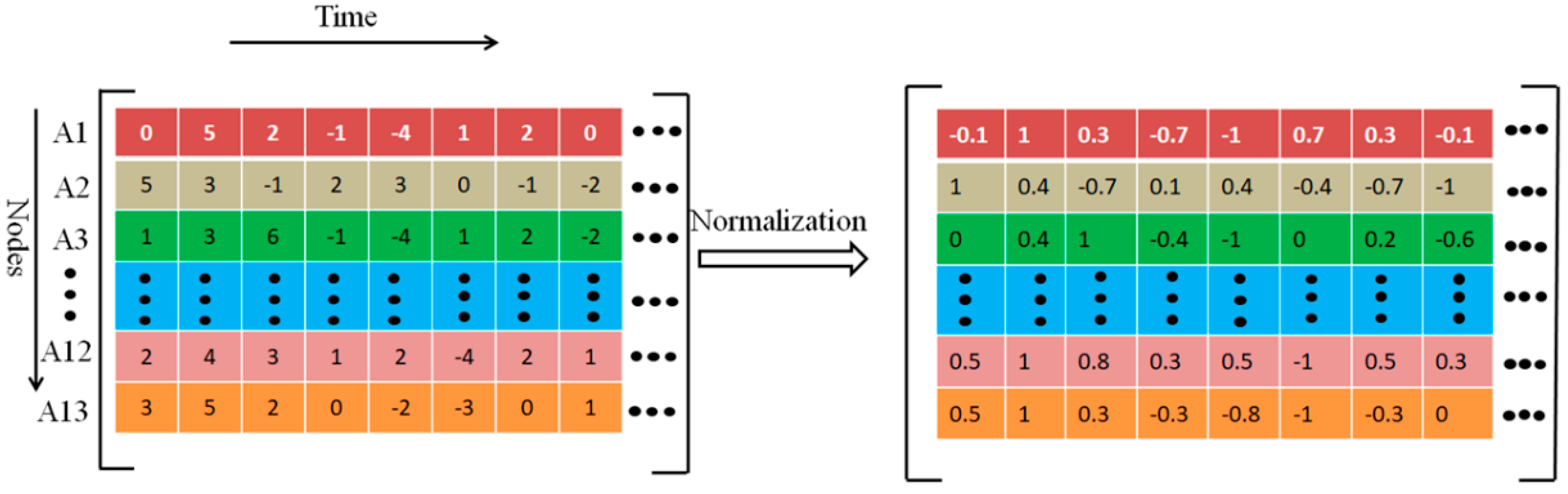
2.3. CNN Samples
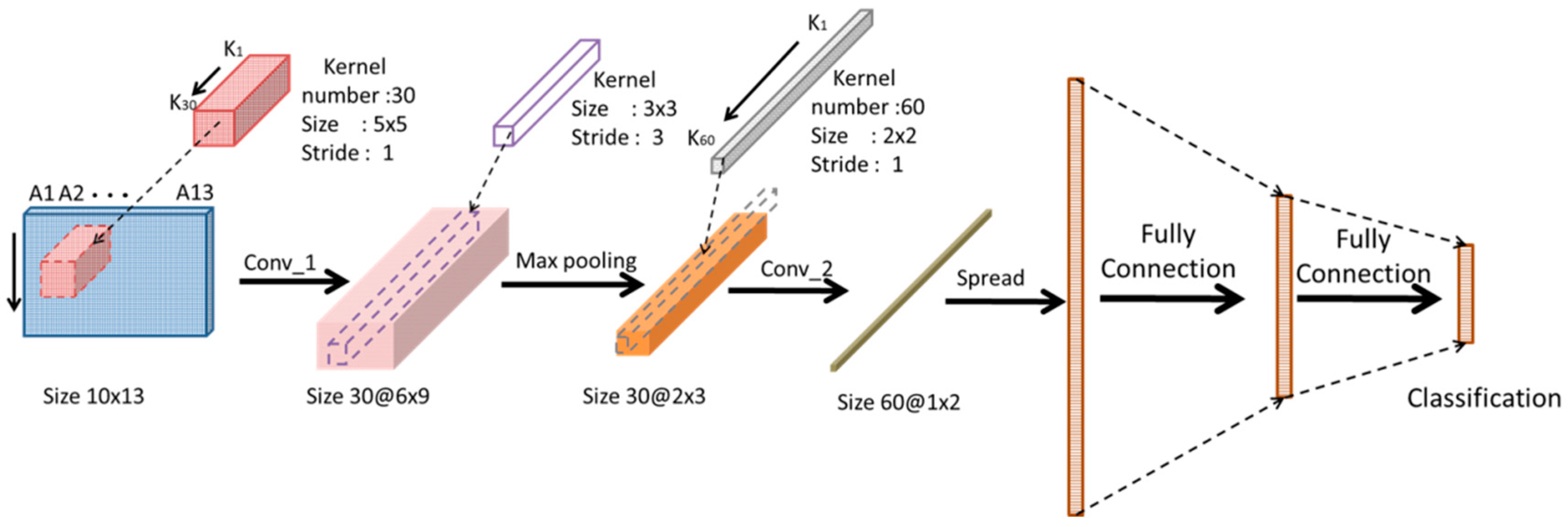
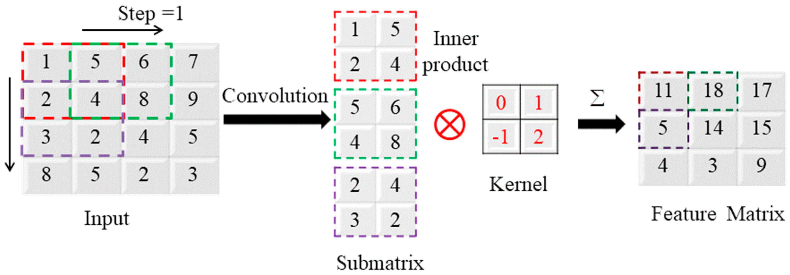
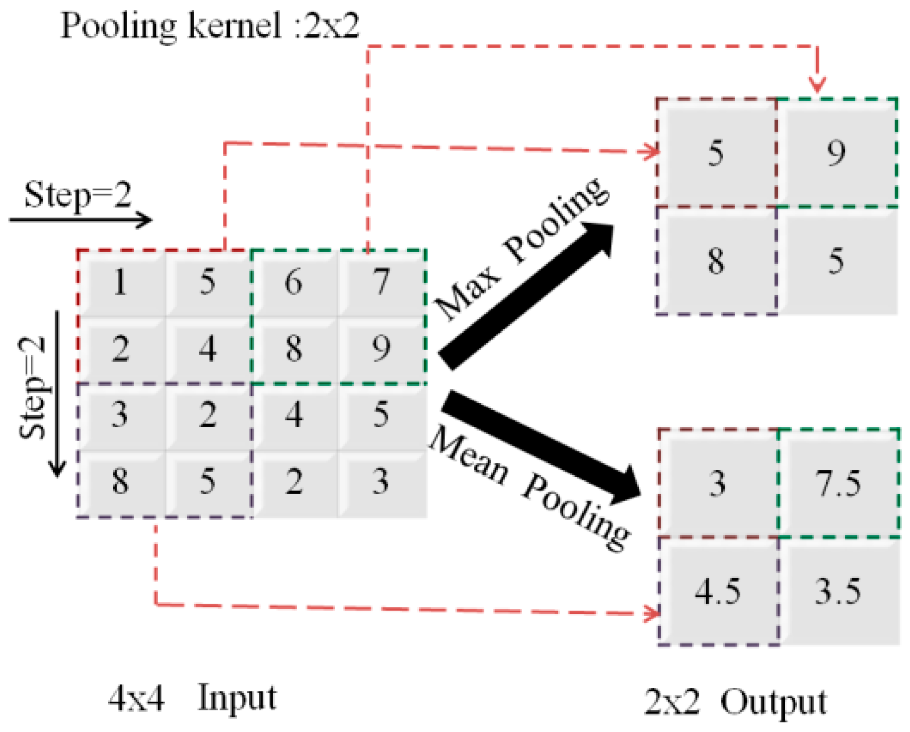
2.4. Convolutional Neural Network
2.5. Structural Damage Detection
3. Results
3.1. Damage Classification Based on Numerical Simulations
3.2. Structural Damage Classification under Vibration Experiments
4. Discussion and Conclusions
Author Contributions
Funding
Conflicts of Interest
References
- Das, S.; Saha, P.; Patro, S.K. Vibration-based damage detection techniques used for health monitoring of structures: A review. J. Civ. Struct. Health Monit. 2016, 6, 477–507. [Google Scholar] [CrossRef]
- Chang, K.C.; Kim, C.W. Modal-parameter identification and vibration-based damage detection of a damaged steel truss bridge. Eng. Struct. 2016, 122, 156–173. [Google Scholar] [CrossRef]
- Farahani, R.V.; Penumadu, D. Damage identification of a full-scale five-girder bridge using time-series analysis of vibration data. Eng. Struct. 2016, 115, 129–139. [Google Scholar] [CrossRef]
- Pandey, A.K.; Biswas, M.; Samman, M.M. Damage detection from changes in curvature mode shapes. J. Sound Vib. 1991, 145, 321–332. [Google Scholar] [CrossRef]
- Salawu, O.S. Detection of structural damage through changes in frequency: A review. Eng. Struct. 1997, 19, 718–723. [Google Scholar] [CrossRef]
- Cawley, P.; Adams, R.D. The location of defects in structures from measurements of natural frequencies. J. Strain Anal. Eng. Des. 1979, 14, 49–57. [Google Scholar] [CrossRef]
- Chen, Y.; Hou, X.B.; Li, W.; Zhang, X.H. Applications of different criteria in structural damage identification based on natural frequency and static displacement. Sci. China Technol. Sci. 2016, 59, 1746. [Google Scholar]
- Döhler, M.; Hille, F.; Mevel, L.; Rücker, W. Structural health monitoring with statistical methods during progressive damage test of S101 Bridge. Eng. Struct. 2014, 69, 183–193. [Google Scholar] [CrossRef]
- Dutta, A.; Talukdar, S. Damage detection in bridges using accurate modal parameters. Finite Elem. Anal. Des. 2004, 40, 287–304. [Google Scholar] [CrossRef]
- Sung, S.H.; Koo, K.Y.; Jung, H.J. Modal flexibility-based damage detection of cantilever beam-type structures using baseline modification. J. Sound Vib. 2014, 333, 4123–4138. [Google Scholar] [CrossRef]
- Cha, Y.; Buyukozturk, O. Structural Damage Detection Using Modal Strain Energy and Hybrid Multiobjective Optimization. Comput.-Aided Civ. Infrastruct. Eng. 2015, 30, 347–358. [Google Scholar] [CrossRef]
- Hou, Z.; Noori, M.; Amand, R.S. Wavelet-Based Approach for Structural Damage Detection. J. Eng. Mech. 2000, 126, 677–683. [Google Scholar] [CrossRef]
- Li, Z.; Park, H.S.; Adeli, H. New method for modal identification of super high-rise building structures using discretized synchrosqueezed wavelet and Hilbert transforms. Struct. Des. Tall Spec. Build. 2017, 26, e1312. [Google Scholar] [CrossRef]
- Tibaduiza, D.A.; Torres-Arredondo, M.A.; Mujica, L.E.; Rodellar, J.; Fritzen, C.P. A study of two unsupervised data driven statistical methodologies for detecting and classifying damages in structural health monitoring. Mech. Syst. Signal Process. 2013, 41, 467–484. [Google Scholar] [CrossRef]
- Ghiasi, R.; Ghasemi, M.R. Optimization-based method for structural damage detection with consideration of uncertainties- a comparative study. Smart Struct. Syst. 2018, 22, 561–574. [Google Scholar]
- Chen, S.; Lin, B.; Han, X.; Liang, X. Automated inspection of engineering ceramic grinding surface damage based on image recognition. Int. J. Adv. Manuf. Technol. 2013, 66, 431–443. [Google Scholar] [CrossRef]
- Screen efficiency comparisons of decision tree and neural network algorithms in machine learning assisted drug design. Sci. China 2019, 62, 110–118.
- Lee, J.J.; Lee, J.W.; Yi, J.H.; Yun, C.B.; Jung, H.Y. Neural networks-based damage detection for bridges considering errors in baseline finite element models. J. Sound Vib. 2005, 280, 555–578. [Google Scholar] [CrossRef]
- Hakim, S.J.S.; Razak, H.A. Structural damage detection of steel bridge girder using artificial neural networks and finite element models. Steel Compos. Struct. 2013, 14, 367–377. [Google Scholar] [CrossRef]
- Zang, C.; Imregun, M. Structural damage detection using artificial neural networks and measured frf data reduced via principal component projection. J. Sound Vib. 2001, 242, 813–827. [Google Scholar] [CrossRef]
- Yao, X. Evolutionary artificial neural networks. Int. J. Neural Syst. 1993, 4, 203–222. [Google Scholar] [CrossRef] [PubMed]
- Yao, W.S. The Researching Overview of Evolutionary Neural Networks. Comput. Sci. 2004, 31, 125–129. [Google Scholar]
- Koziarski, M.; Cyganek, B. Image recognition with deep neural networks in presence of noise-Dealing with and taking advantage of distortions. Integr. Comput.-Aided Eng. 2017, 24, 1–13. [Google Scholar] [CrossRef]
- Simonyan, K.; Zisserman, A. Very Deep Convolutional Networks for Large-Scale Image Recognition. arXiv 2014, arXiv:1409.1556. [Google Scholar]
- Cha, Y.; Choi, W.; Büyüköztürk, O. Deep Learning-Based Crack Damage Detection Using Convolutional Neural Networks. Comput.-Aided Civ. Infrastruct. Eng. 2017, 32, 361–378. [Google Scholar] [CrossRef]
- Lin, Y.Z.; Nie, Z.H.; Ma, H.W. Structural Damage Detection with Automatic Feature extraction through Deep Learning. Comput.-Aided Civ. Infrastruct. Eng. 2017, 32, 1–22. [Google Scholar] [CrossRef]
- Abdeljaber, O.; Avci, O.; Kiranyaz, S.; Gabbouj, M.; Inman, D.J. Real-time vibration-based structural damage detection using one-dimensional convolutional neural networks. J. Sound Vib. 2017, 388, 154–170. [Google Scholar] [CrossRef]
- Zhang, Y.; Miyamori, Y.; Mikami, S.; Saito, T. Vibration-based structural state identification by a 1-dimensional convolutional neural network. Comput.-Aided Civ. Infrastruct. Eng. 2019, 34, 1–18. [Google Scholar] [CrossRef]
- Teng, S.; Chen, G.; Gong, P.; Liu, G.; Cui, F. Structural damage detection using convolutional neural networks combining strain energy and dynamic response. Meccanica 2019, 55, 945–959. [Google Scholar] [CrossRef]
- Scherer, D.; Müller, A.; Behnke, S. Evaluation of Pooling Operations in Convolutional Architectures for Object Recognition. In Proceedings of the International Conference on Artificial Neural Networks, Thessaloniki, Greece, 15–18 September 2010. [Google Scholar]
- Krizhevsky, A.; Sutskever, I.; Hinton, G.E. ImageNet Classification with Deep Convolutional Neural Networks. In Proceedings of the International Conference on Neural Information Processing Systems, Lake Tahoe, NV, USA, 3–6 December 2012; pp. 1097–1105. [Google Scholar]
- Kingma, D.; Ba, J. Adam: A Method for Stochastic Optimization. arXiv 2014, arXiv:1412.6980. [Google Scholar]
- García-Macías, E.; Ubertini, F. MOVA/MOSS: Two integrated software solutions for comprehensive Structural Health Monitoring of structures. Mech. Syst. Signal Process. 2020, 143, 106830. [Google Scholar] [CrossRef]
- Kita, A.; Cavalagli, N.; Ubertini, F. Temperature effects on static and dynamic behavior of Consoli Palace in Gubbio, Italy. Mech. Syst. Signal Process. 2019, 120, 180–202. [Google Scholar] [CrossRef]


| Datasets | Damage Scenarios | Samples | Total |
|---|---|---|---|
| A | State 0 | 15,991 | 159,910 |
| State 1 | 15,991 | ||
| … | … | ||
| … | … | ||
| State 9 | 15,991 | ||
| B | State 1 | 15,991 | |
| State 2 | 15,991 | ||
| … | … | 575,676 | |
| … | … | ||
| State 36 | 15,991 | ||
| C | State 1 | 15,991 | |
| State 2 | 15,991 | ||
| … | … | 1,343,244 | |
| … | … | ||
| State 83 | 15,991 | ||
| State 84 | 15,991 |
| Damage Scenarios | Samples | Damage Scenarios | Samples |
|---|---|---|---|
| State 0 | 15,991 | State 4 | 15,991 |
| State 1 | 15,991 | State 5 | 15,991 |
| State 2 | 15,991 | State 6 | 15,991 |
| State 3 | 15,991 | State 7 | 15,991 |
| Total | 127,928 |
| Damage Scenarios | Samples | Damage Scenarios | Samples |
|---|---|---|---|
| State 0 | 791 | State 4 | 791 |
| State 1 | 791 | State 5 | 791 |
| State 2 | 791 | State 6 | 791 |
| State 3 | 791 | State 7 | 791 |
| Total | 6328 |
| Layer | Type | Kernel Number | Kernel Size | Stride | Padding | Activation |
|---|---|---|---|---|---|---|
| 1 | Input | None | None | None | None | None |
| 2 | Convolution | 30 | [5 5] | [1 1] | 0 | ReLU |
| 3 | Max Pooling | None | [3 3] | [3 3] | 0 | None |
| 4 | Convolution | 60 | [2 2] | [1 1] | 0 | ReLU |
| 5 | FC | None | None | None | None | None |
| 6 | Softmax | None | None | None | None | None |
| 7 | Output | None | None | None | None | None |
| Amount | Prediction Damage Location | ||||||||||||
|---|---|---|---|---|---|---|---|---|---|---|---|---|---|
| 0 | 1 | 2 | 3 | 4 | 5 | 6 | 7 | 8 | 9 | Total | % | ||
| Actual damage location | 0 | 675 | 10 | 0 | 0 | 65 | 0 | 0 | 41 | 0 | 0 | 791 | 85.3 |
| 1 | 5 | 766 | 0 | 0 | 14 | 0 | 0 | 4 | 2 | 0 | 791 | 96.8 | |
| 2 | 0 | 0 | 791 | 0 | 0 | 0 | 0 | 0 | 0 | 0 | 791 | 100 | |
| 3 | 0 | 0 | 2 | 789 | 0 | 0 | 0 | 0 | 0 | 0 | 791 | 99.7 | |
| 4 | 40 | 27 | 0 | 0 | 724 | 0 | 0 | 0 | 0 | 0 | 791 | 91.5 | |
| 5 | 0 | 0 | 0 | 0 | 0 | 791 | 0 | 0 | 0 | 0 | 791 | 100 | |
| 6 | 0 | 0 | 0 | 0 | 1 | 0 | 790 | 0 | 0 | 0 | 791 | 99.9 | |
| 7 | 66 | 5 | 0 | 0 | 31 | 0 | 0 | 689 | 0 | 0 | 791 | 87.1 | |
| 8 | 2 | 1 | 0 | 0 | 0 | 0 | 0 | 0 | 788 | 0 | 791 | 99.6 | |
| 9 | 0 | 0 | 0 | 0 | 0 | 0 | 0 | 0 | 0 | 791 | 791 | 100 | |
| Total | 788 | 809 | 793 | 789 | 835 | 791 | 790 | 734 | 790 | 791 | 7910 | 96 | |
| Damage State | Predicted Number | Total | % | Damage State | Predicted Number | Total | % |
|---|---|---|---|---|---|---|---|
| 1 | 726 | 791 | 91.8 | 19 | 715 | 791 | 90.4 |
| 2 | 744 | 791 | 94.1 | 20 | 780 | 791 | 98.6 |
| 3 | 715 | 791 | 90.4 | 21 | 783 | 791 | 99.0 |
| 4 | 754 | 791 | 95.3 | 22 | 736 | 791 | 93.0 |
| 5 | 727 | 791 | 91.9 | 23 | 726 | 791 | 91.8 |
| 6 | 727 | 791 | 91.9 | 24 | 752 | 791 | 95.1 |
| 7 | 697 | 791 | 88.1 | 25 | 727 | 791 | 91.9 |
| 8 | 727 | 791 | 91.9 | 26 | 700 | 791 | 88.5 |
| 9 | 783 | 791 | 99.0 | 27 | 781 | 791 | 98.7 |
| 10 | 721 | 791 | 91.2 | 28 | 727 | 791 | 91.9 |
| 11 | 778 | 791 | 98.4 | 29 | 788 | 791 | 99.6 |
| 12 | 773 | 791 | 97.7 | 30 | 776 | 791 | 98.1 |
| 13 | 732 | 791 | 92.5 | 31 | 712 | 791 | 90.0 |
| 14 | 783 | 791 | 99.0 | 32 | 787 | 791 | 99.5 |
| 15 | 779 | 791 | 98.5 | 33 | 783 | 791 | 99.0 |
| 16 | 745 | 791 | 94.2 | 34 | 736 | 791 | 93.0 |
| 17 | 780 | 791 | 98.6 | 35 | 697 | 791 | 88.1 |
| 18 | 773 | 791 | 97.7 | 36 | 790 | 791 | 99.9 |
| Total | 94.6 |
| Damage State | Predicted Number | Total | % | Damage State | Predicted Number | Total | % |
|---|---|---|---|---|---|---|---|
| 1 | 758 | 791 | 95.8 | 43 | 788 | 791 | 99.6 |
| 2 | 714 | 791 | 90.3 | 44 | 707 | 791 | 89.4 |
| 3 | 769 | 791 | 97.2 | 45 | 784 | 791 | 99.1 |
| 4 | 754 | 791 | 95.3 | 46 | 788 | 791 | 99.6 |
| 5 | 754 | 791 | 95.3 | 47 | 753 | 791 | 95.2 |
| 6 | 748 | 791 | 94.6 | 48 | 732 | 791 | 92.5 |
| 7 | 741 | 791 | 93.7 | 49 | 790 | 791 | 99.9 |
| 8 | 744 | 791 | 94.1 | 50 | 733 | 791 | 92.7 |
| 9 | 756 | 791 | 95.6 | 51 | 768 | 791 | 97.1 |
| 10 | 756 | 791 | 95.6 | 52 | 760 | 791 | 96.1 |
| 11 | 750 | 791 | 94.8 | 53 | 765 | 791 | 96.7 |
| 12 | 755 | 791 | 95.4 | 54 | 767 | 791 | 97.0 |
| 13 | 756 | 791 | 95.6 | 55 | 786 | 791 | 99.4 |
| 14 | 730 | 791 | 92.3 | 56 | 767 | 791 | 97.0 |
| 15 | 727 | 791 | 91.9 | 57 | 790 | 791 | 99.9 |
| 16 | 788 | 791 | 99.6 | 58 | 785 | 791 | 99.2 |
| 17 | 704 | 791 | 89.0 | 59 | 722 | 791 | 91.3 |
| 18 | 745 | 791 | 94.2 | 60 | 788 | 791 | 99.6 |
| 19 | 750 | 791 | 94.8 | 61 | 791 | 791 | 100.0 |
| 20 | 763 | 791 | 96.5 | 62 | 744 | 791 | 94.1 |
| 21 | 776 | 791 | 98.1 | 63 | 732 | 791 | 92.5 |
| 22 | 765 | 791 | 96.7 | 64 | 791 | 791 | 100.0 |
| 23 | 743 | 791 | 93.9 | 65 | 755 | 791 | 95.4 |
| 24 | 755 | 791 | 95.4 | 66 | 756 | 791 | 95.6 |
| 25 | 742 | 791 | 93.8 | 67 | 747 | 791 | 94.4 |
| 26 | 742 | 791 | 93.8 | 68 | 743 | 791 | 93.9 |
| 27 | 697 | 791 | 88.1 | 69 | 767 | 791 | 97.0 |
| 28 | 762 | 791 | 96.3 | 70 | 763 | 791 | 96.5 |
| 29 | 745 | 791 | 94.2 | 71 | 750 | 791 | 94.8 |
| 30 | 789 | 791 | 99.7 | 72 | 778 | 791 | 98.4 |
| 31 | 781 | 791 | 98.7 | 73 | 758 | 791 | 95.8 |
| 32 | 749 | 791 | 94.7 | 74 | 775 | 791 | 98.0 |
| 33 | 791 | 791 | 100.0 | 75 | 744 | 791 | 94.1 |
| 34 | 791 | 791 | 100.0 | 76 | 789 | 791 | 99.7 |
| 35 | 750 | 791 | 94.8 | 77 | 789 | 791 | 99.7 |
| 36 | 758 | 791 | 95.8 | 78 | 728 | 791 | 92.0 |
| 37 | 773 | 791 | 97.7 | 79 | 736 | 791 | 93.0 |
| 38 | 762 | 791 | 96.3 | 80 | 785 | 791 | 99.2 |
| 39 | 759 | 791 | 96.0 | 81 | 737 | 791 | 93.2 |
| 40 | 789 | 791 | 99.7 | 82 | 759 | 791 | 96.0 |
| 41 | 746 | 791 | 94.3 | 83 | 791 | 791 | 100.0 |
| 42 | 791 | 791 | 100.0 | 84 | 690 | 791 | 87.2 |
| Total | 95.8 |
| Amount | Prediction Damage Location | ||||||||||
|---|---|---|---|---|---|---|---|---|---|---|---|
| 0 | 1 | 2 | 3 | 4 | 5 | 6 | 7 | Total | % | ||
| Actual damage location | 0 | 773 | 0 | 16 | 0 | 2 | 0 | 0 | 0 | 791 | 97.7 |
| 1 | 0 | 770 | 1 | 0 | 0 | 20 | 0 | 0 | 791 | 97.3 | |
| 2 | 32 | 0 | 757 | 0 | 2 | 0 | 0 | 0 | 791 | 95.7 | |
| 3 | 0 | 0 | 1 | 774 | 16 | 0 | 0 | 0 | 791 | 97.9 | |
| 4 | 2 | 0 | 0 | 49 | 740 | 0 | 0 | 0 | 791 | 93.6 | |
| 5 | 0 | 33 | 0 | 0 | 0 | 758 | 0 | 0 | 791 | 95.8 | |
| 6 | 3 | 1 | 0 | 0 | 0 | 0 | 787 | 0 | 791 | 99.5 | |
| 7 | 0 | 0 | 0 | 0 | 0 | 0 | 0 | 791 | 791 | 100 | |
| Total | 810 | 804 | 775 | 823 | 760 | 778 | 787 | 791 | 6328 | 97.2 | |
| Amount | Prediction Damage Location | ||||||||||
|---|---|---|---|---|---|---|---|---|---|---|---|
| 0 | 1 | 2 | 3 | 4 | 5 | 6 | 7 | Total | % | ||
| Actual damage location | 0 | 742 | 4 | 33 | 0 | 12 | 0 | 0 | 0 | 791 | 93.8 |
| 1 | 41 | 687 | 9 | 0 | 0 | 54 | 0 | 0 | 791 | 86.9 | |
| 2 | 56 | 17 | 691 | 7 | 20 | 0 | 0 | 0 | 791 | 87.3 | |
| 3 | 15 | 0 | 19 | 702 | 45 | 10 | 0 | 0 | 791 | 88.7 | |
| 4 | 27 | 0 | 7 | 78 | 679 | 0 | 0 | 0 | 791 | 85.8 | |
| 5 | 9 | 69 | 2 | 8 | 0 | 693 | 10 | 0 | 791 | 87.6 | |
| 6 | 0 | 12 | 0 | 0 | 0 | 38 | 741 | 0 | 791 | 93.6 | |
| 7 | 0 | 0 | 0 | 0 | 0 | 5 | 21 | 765 | 791 | 96.7 | |
| All | 890 | 789 | 761 | 795 | 756 | 800 | 772 | 765 | 6328 | 90.1 | |
© 2020 by the authors. Licensee MDPI, Basel, Switzerland. This article is an open access article distributed under the terms and conditions of the Creative Commons Attribution (CC BY) license (http://creativecommons.org/licenses/by/4.0/).
Share and Cite
Teng, Z.; Teng, S.; Zhang, J.; Chen, G.; Cui, F. Structural Damage Detection Based on Real-Time Vibration Signal and Convolutional Neural Network. Appl. Sci. 2020, 10, 4720. https://doi.org/10.3390/app10144720
Teng Z, Teng S, Zhang J, Chen G, Cui F. Structural Damage Detection Based on Real-Time Vibration Signal and Convolutional Neural Network. Applied Sciences. 2020; 10(14):4720. https://doi.org/10.3390/app10144720
Chicago/Turabian StyleTeng, Zhiqiang, Shuai Teng, Jiqiao Zhang, Gongfa Chen, and Fangsen Cui. 2020. "Structural Damage Detection Based on Real-Time Vibration Signal and Convolutional Neural Network" Applied Sciences 10, no. 14: 4720. https://doi.org/10.3390/app10144720
APA StyleTeng, Z., Teng, S., Zhang, J., Chen, G., & Cui, F. (2020). Structural Damage Detection Based on Real-Time Vibration Signal and Convolutional Neural Network. Applied Sciences, 10(14), 4720. https://doi.org/10.3390/app10144720