Bridge Crack Detection Based on SSENets

Abstract

Bridge crack detection is essential to prevent transportation accidents. However, the surrounding environment has great interference with the detection of cracks, which makes it difficult to ensure the accuracy of the detection. In order to accurately detect bridge cracks, we proposed an end-to-end model named Skip-Squeeze-and-Excitation Networks (SSENets). It is mainly composed of the Skip-Squeeze-Excitation (SSE) module and the Atrous Spatial Pyramid Pooling (ASPP) module. The SSE module uses skip-connection strategy to enhance the gradient correlation between the shallow network and deeper network, alleviating the vanishing gradient caused by the deepening of the network. The ASPP module can extract multi-scale contextual information of images, while the depthwise separable convolution reduces computational complexity. In order to avoid destroying the topology of crack, we used atrous convolution instead of the pooling layer. The proposed SSENets achieved a detection accuracy of 97.77%, which performed better than the models we compared it with. The designed SSE module which used skip-connection strategy can be embedded in other convolutional neural networks (CNNs) to improve their performance.

1. Introduction

In modern society, it is important to ensure the safety of bridges. Crack is one of the most common diseases of bridge structures, so detecting and repairing cracks in time are important tasks for the maintenance of bridges [1]. It can effectively prevent bridge quality problems from endangering transportation safety. In view of the strict requirements for bridge safety, we have to detect tiny cracks successfully and overcome the interference of noise, scratches and uneven illumination to the detection results. Workers used to rely on subjective judgment to detect bridge cracks, which would cause the problems of low efficiency, accuracy and be time consuming, thus it is not appropriate for actual application. With an advancement in computer vision and deep learning techniques, computer vision has been applied in the field of crack detection [2,3], solving the problem of crack detection methods in recent decades.

In recent years, crack detection algorithms based on computer vision are being continuously developed. Threshold segmentation [4], morphological [5], wavelet transform [6], and the filter-based algorithm [7] have been applied to detect cracks. Although these algorithms may achieve high detection accuracy after adjusting parameters, they are only effective for images captured in specific environments. In other words, when the illumination and shooting distance change, the parameters need to be adjusted to ensure the high detection accuracy.

To satisfy the requirement of working in different environments, we considered the use of convolutional neural networks (CNNs) to detect bridge cracks. CNNs was first proposed by LeCun et al. [8]. It was widely used in image classification [9,10,11,12], object detection [13], and action recognition [14] due to the outstanding learning capability. The deeper network in CNNs can further extract the feature of feature map, which is obtained by shallow network. Influenced by this characteristic of CNNs, researchers have been devoted to the field of pixel-level crack detection. CrackNet [15] was applied to crack detection in 2017. Unlike the traditional CNN structure, it removed pooling layers to avoid loss of detail due to over downsampling. Though high detection accuracy can be achieved, the feature generator used in CrackNet produced handcrafted features using predesigned line filters, which leads to the limitations in learning capability. CrackNet-V [16] was modified on the basis of CrackNet, and it had a deeper structure and fewer parameters. At the same time, CrackNet-V improved detection efficiency and reduced calculation cast. CrackSeg [17] and U-Net [18] can also get high detection accuracy. However, like other pixel-level crack detection algorithms, they need to label each pixel of each image in the datasets, so the production of the datasets is a complex project. Meanwhile, the large number of parameters and long training time of pixel-level crack detection make it less feasible in practical engineering.

In order to meet the fast and accurate requirements in crack detection task, researchers have designed classifiers to judge whether the image cells are cracks. Artificial Neural Networks (ANNs) [19,20,21] and Support Vector Machines (SVMs) [22,23] have been verified to perform classifications on crack detection. However, these techniques generally represent only a few layers of abstraction and could not fully understand the complexity of bridge surface [16]. Cha et al. [24] proposed a network based on CNNs and combined with the sliding window technique, which can detect images with a resolution greater than 256 × 256 pixels. Xu et al. [25] designed an end-to-end model based on the Atrous Spatial Pyramid Pooling (ASPP) module, achieving a detection accuracy of 96.37%. Although these methods could complete the task of crack detection, the accuracy and computational complexity of the detection can be further improved.

The conventional convolution used in the above studies is aggregated simultaneously in the spatial dimension and the channel dimension of the feature map, which ignores the relationship between channels and fails to establish the connections among the channels. Therefore, it would block the network from studying the features of images. In order to deal with the problem of high complexity and low detection accuracy in the conventional convolution, Inception [26,27,28,29], Xception [30], MobileNet [31], Squeeze-and-Excitation Networks (SENets) [32] used depthwise separable convolution, separating the aggregation in spatial dimension and channel dimension. These methods verified that the depthwise separable convolution can improve the performance of the network while reducing the parameters of the model. Compared with other networks, SENets used global information to establish the relationship among channels, and recalibrated the value of the feature map. Though it could improve the network performance, if the input of the SE module is a single feature map, the network performance will be greatly reduced when the vanishing gradient appears with the increase of network depth.

In order to solve above problems, we proposed a convolutional neural network named Skip-Squeeze-and-Excitation Networks (SSENets), which based on the embedded SSE module. Our main contributions are as follows:

• We designed an embedded module with skip-connection strategy, which was called Skip-Squeeze-and-Excitation (SSE) module. By inserting the SSE module into the existing network, the detection accuracy can be improved without increasing the computational complexity.
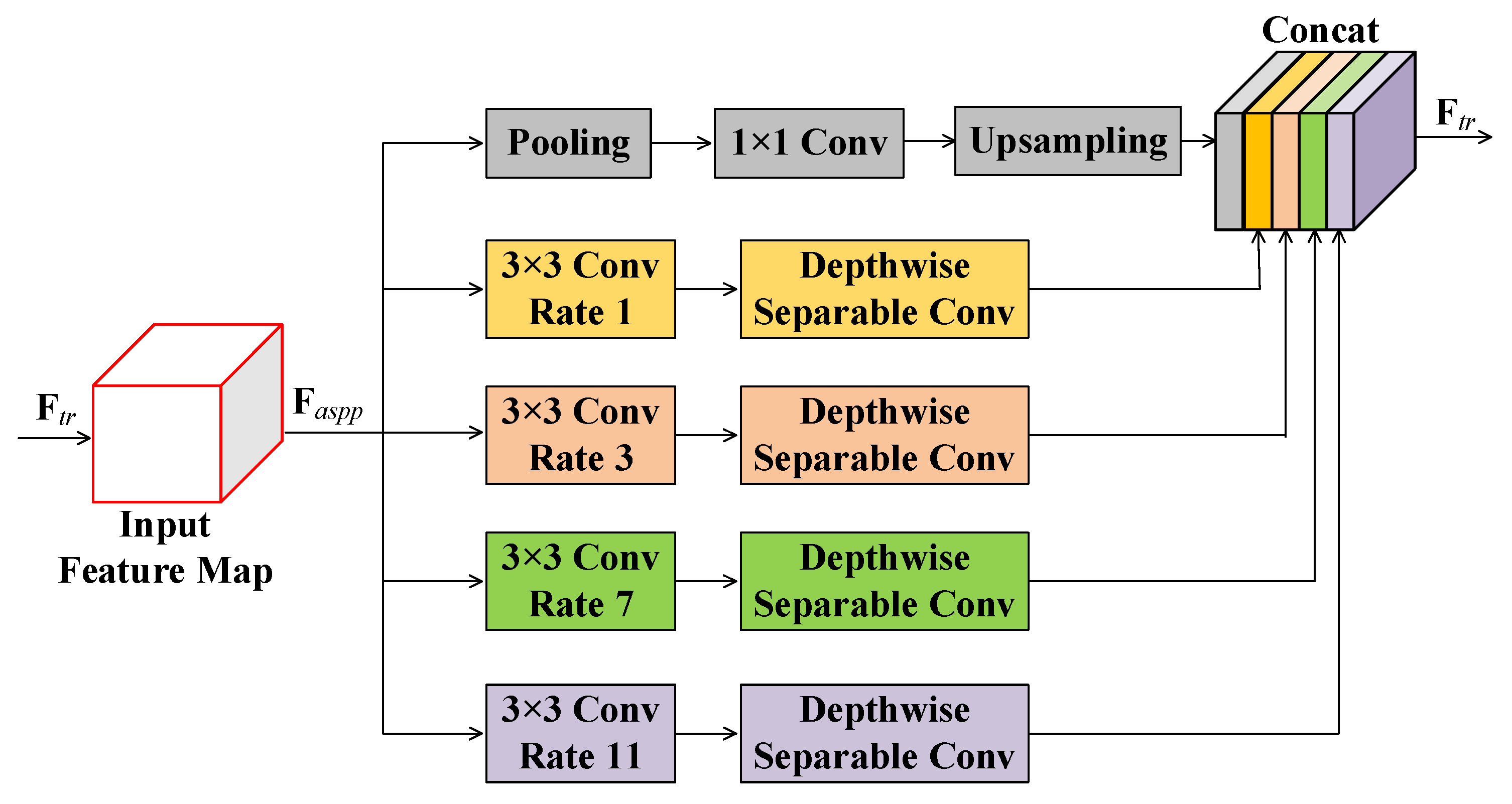
• Considering the large span of crack size in the crack detection task, we introduced the Atrous Spatial Pyramid Pooling (ASPP) module into our model. It can effectively improve the detection accuracy by capturing the context of images in multiple scales.
• Based on the above-mentioned modules, we proposed SSENets, which was applied to the bridge crack detection task. The detection accuracy of SSENets can reach 97.77%, which is higher than the traditional classification models and the model proposed by Xu et al. [25] under the same model complexity.

2. Materials and Methods

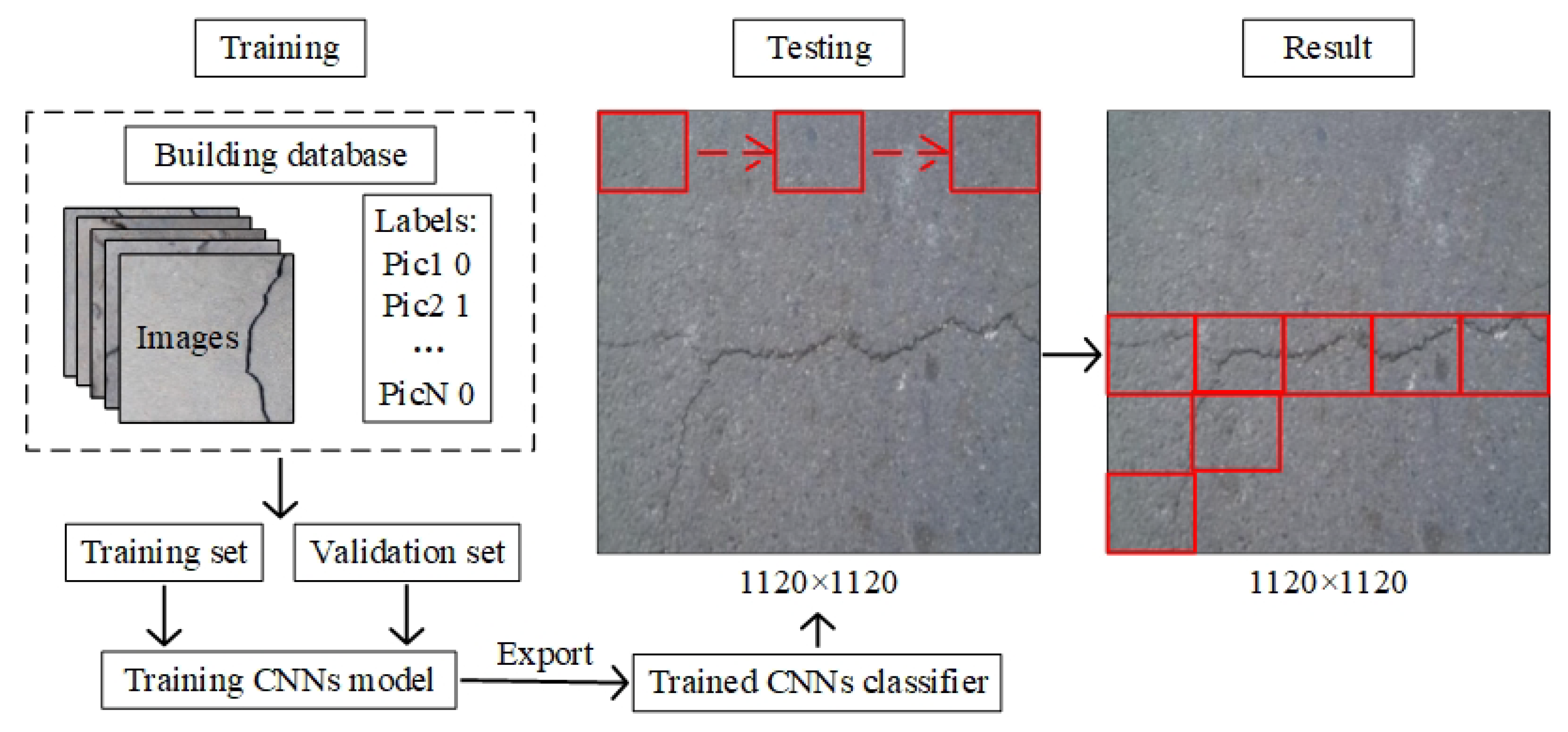
2.1. Datasets

In order to meet the experimental requirements, we used the bridge crack dataset created by Xu et al. [25] as input for training and testing. A total of 2068 initial images of the dataset were collected by Phantom 4 Pro’s Complementary Metal Oxide Semiconductor (CMOS) surface array camera with a resolution of 1024 × 1024. In order to construct positive samples (images with cracks) and negative samples (images without cracks), the initial images were divided into four parts. Sub images were filtered, cropped and flipped, then 6069 images with resolution of 224 × 224 were obtained. The combination of images and labels was used as the dataset. We chose 4856 images as the training set and 1213 images as the testing set. As shown in Figure 1, the flow chart of the crack detection task was divided into two parts: training and testing. By inputting the training set into SSENets, we can get a trained crack classifier. It can be used to detect whether there are cracks in the testing set, and finally get the output of the task. In the test, we used the sliding window technique to traverse the whole image. The structure of SSENets will be described in detail below.

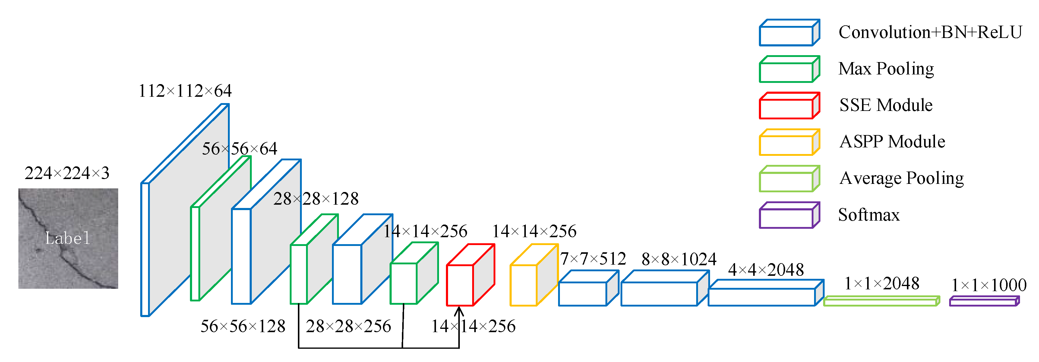
2.2. Proposed Network

In order to improve the capability of the model, reduce the model complexity and alleviate the vanishing gradient in the training process, we proposed a model named SSENets, based on the SSE module using skip-connection strategy and the ASPP module using atrous convolutions with multi-sample rates. The structure of SSENets is shown in Figure 2, which contains the core SSE module, ASPP module and conventional convolutional layers and pooling layers. The role of the first three convolutional layers is to extract the images features. The module takes the feature maps from the second and third convolutional layers as the input of the SSE module, and uses the generated channel weights to recalibrate the feature map. The SSE module uses feature maps from different layers as input, which can improve the problem of the vanishing gradient in the training process. The structure of SSE module will be detailed in Section 2.3. So as to improve the learning capability to cracks features, the model takes the output feature map of SSE module as the input of ASPP module and extracts the multi-scale features. We structure the ASPP module with depthwise separable convolution in order to greatly reduce the parameters and model complexity. The structure of ASPP module will be detailed in Section 2.4. In addition, in order to avoid destroying the topology of the cracks after using several pooling layers to sample the feature map, we introduce atrous convolution with an atrous rate of 2 in the last three convolutional layers. Finally, we use the Softmax function to predict whether the input images contain cracks or not.

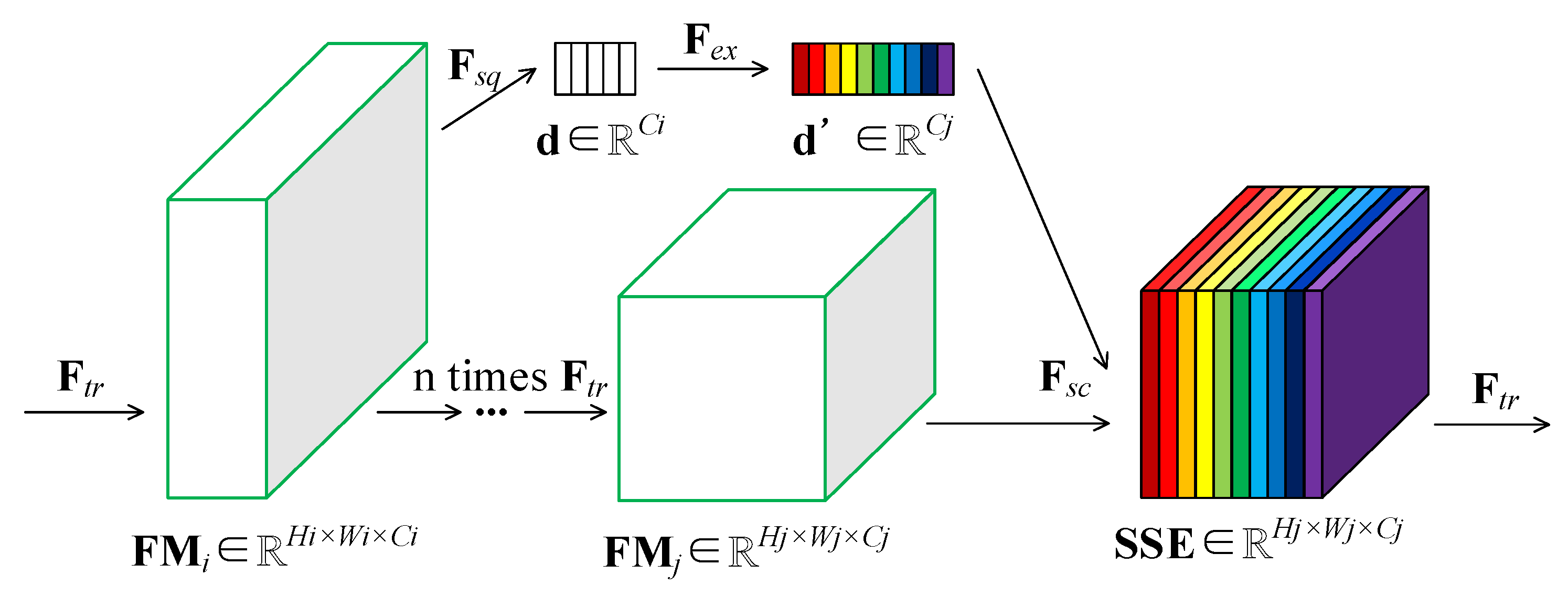
2.3. Skip-Squeeze-and-Excitation Module

To alleviate the vanishing gradient problem with the increase of the depth of the model, we design the embedded SSE module based on the skip-connection strategy, the structure of which is shown in Figure 3. ${\mathrm{F}}_{tr}$ refers to any matrix transformation in the network. The feature map ${\mathrm{FM}}_i\in {ℝ}^{H_i\times W_i\times C_i}$ can be obtained by ${\mathrm{F}}_{tr}$, where $i\le n$, $n$ is the total number of convolutional layers in the network. ${\mathrm{F}}_{sq}$ represents the squeeze operator in the SSE module. The input of the Squeeze operation is the feature map ${\mathrm{FM}}_i$, and its spatial dimensions of each channel will be aggregated to get the channel-wise descriptor $\mathrm{d}\in {ℝ}^{C_i}$. ${\mathrm{F}}_{ex}$ represents the excitation operator in the SSE module. The excitation operator maps the input channel-wise descriptor $\mathrm{d}$ to a set of channel weights $\mathrm{d}\prime \in {ℝ}^{C_j}$, the channel number of which is the same as the output feature map ${\mathrm{FM}}_j\in {ℝ}^{H_j\times W_j\times C_j}$. Then select the feature map ${\mathrm{FM}}_j\in {ℝ}^{H_j\times W_j\times C_j}$ obtained by the j-th convolutional layer, multiply with channel weights $\mathrm{d}\prime$. During the training process, the channel weight $\mathrm{d}\prime$ is adjusted continuously, and each channel of ${\mathrm{FM}}_j$ is recalibrated, so as to enhance the learning capability of the module.

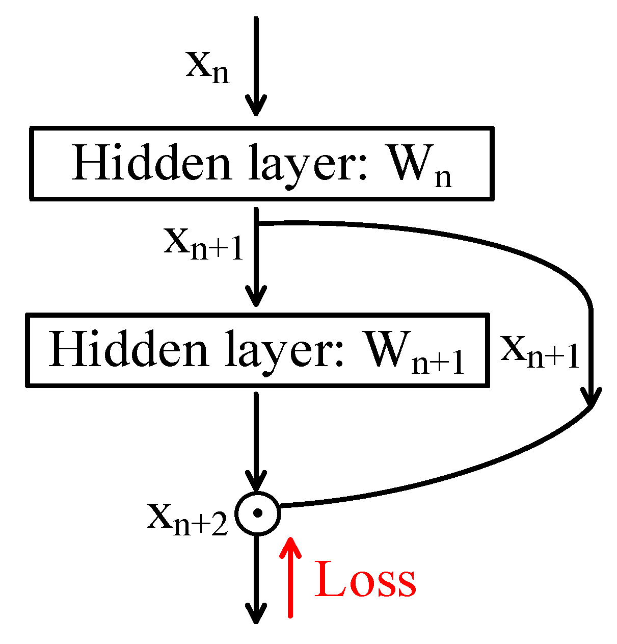
2.3.1. Skip-Connection

The appearance of VGGNets [33] proves that the performance of network increases with the increase of network depth. However, with the increase of network depth, vanishing gradient would appear. The essence that CNNs can iterate continuously is the back propagation of parameters. The chain rule of back propagation will make the gradient less than 1 close to 0 after iteration, so that the parameters far from the output layer cannot be undated. Therefore, it is impossible to increase the number of network layers without limitation in order to improve the network performance.

To alleviate the vanishing gradient caused by the depth increase of the network, this paper designs the SSE module using the skip-connection strategy. SSE module selects the feature map of different depths as input, and uses the channel weight $\mathrm{d}\prime$ generated by the shallow layer to recalibrate the feature map ${\mathrm{FM}}_j$ generated by the deeper layers. This strategy can increase the gradient correlation of the model, and alleviate the vanishing gradient of CNNs with the increase of the depth of the model. Therefore, it makes the model easier to optimize, and improves the detection accuracy. The simplified model of SSE module is shown in Figure 4. We assume that the input of the model is $x_n$, the output is $x_{n+2}$ after two hidden layers. The formula of $x_{n+2}$ is shown in Equation (1):

$$x_{n+2}=x_{n+1}⨀ℱ\left(x_{n+1},W_{n+1}\right),$$

(1)

where $W_n$ represents the parameters of the hidden layer. Operator $⨀$ represents Hadamard product of the matrix. From the chain rule, the partial derivative of loss function $Loss$ to parameter $W_n$ is shown in Equation (2):

$$\frac{\partial Loss}{\partial W_n}=\frac{\partial Loss}{\partial x_{n+2}}·\frac{\partial x_{n+2}}{\partial x_{n+1}}·\frac{\partial x_{n+1}}{\partial W_n}=\frac{\partial Loss}{\partial x_{n+2}}\left[ℱ\left(x_{n+1},W_{n+1}\right)+x_{n+1}·\frac{\partial }{\partial x_{n+1}}ℱ\left(x_{n+1},W_{n+1}\right)\right]\frac{\partial x_{n+1}}{\partial W_n},$$

(2)

It can be seen from the formula that the square brackets contain two items, even if the partial derivative $\frac{\partial }{\partial x_{n+1}}ℱ\left(x_{n+1},W_{n+1}\right)$ approaches 0 with the increase of iteration times and the depth of the model, $\frac{\partial Loss}{\partial W_n}$ won’t be 0. Therefore, our model can alleviate vanishing gradient of the network.

2.3.2. Squeeze

Each pixel obtained from conventional convolution is only related to the context in the local receptive field and cannot take advantage of the context outside the receptive field. To solve this problem, we use the Squeeze operator to aggregate global information into a channel descriptor $\mathrm{d}$. We apply global average pooling to generate a channel-wise vector from the input feature map ${\mathrm{FM}}_i$. It can shrink the context with the size of $H_i\times W_i$ to the size of $1\times 1$ in spatial dimension. The formula of channel descriptor is shown in Equation (3):

$$d_c={\mathrm{F}}_{sq}\left({\mathrm{FM}}_{ci}\right)=\frac{1}{H_i\times W_i}{\displaystyle \sum }_{m=1}^{H_i}{\displaystyle \sum }_{n=1}^{W_i}F{M}_{ic}\left(m,n\right),$$

(3)

where $d_c$ is the value of c-th channel in the channel descriptor $\mathrm{d}$ and $F{M}_{ic}$ refers to the c-th channel of the feature map ${\mathrm{FM}}_i$. We choose the simplest aggregation strategy [32], which can improve the capability of the module while minimizing the complexity of the module.

2.3.3. Excitation

In order to alleviate the vanishing gradient of the network with the increase of the depth of the model, we choose the feature map ${\mathrm{FM}}_j$ from deeper layer interaction with the channel descriptor $\mathrm{d}$ from the shallow feature map. However, the number of channels in ${\mathrm{FM}}_j$ and $\mathrm{d}$ is generally different. To make them possible to be multiplied, we have to post-process the channel descriptor $\mathrm{d}$. Squeeze operator establishes the global information of each channel in spatial dimension, but it does not consider the connection between channels. Therefore, excitation operator adopts the gating strategy [32] to focus on establishing the connection between channels, the formula is shown in Equation (4):

$$\mathrm{d}\prime ={\mathrm{F}}_{ex}\left(\mathrm{d},{\mathrm{W}}_1,{\mathrm{W}}_2\right)=\delta \left({\mathrm{W}}_2\delta \left({\mathrm{W}}_1\mathrm{d}\right)\right),$$

(4)

where $\mathrm{d}\prime =\left[d_1^{\prime },d_2^{\prime },\dots ,d_c^{\prime },\dots ,d_j^{\prime }\right]$, $\delta$ refers to the Rectified Linear Unit (ReLU) activation function [34], ${\mathrm{W}}_1\in {ℝ}^{\frac{C_i}{r}\times C_i}$ and ${\mathrm{W}}_2\in {ℝ}^{C_j\times \frac{C_i}{r}}$, r is reduction ratio. To build up the correlation between channels, we take the channel descriptor $\mathrm{d}$ as the input of two fully-connected layers. According to Equation (4), the first fully-connected layer changes the number of channels from $C_i$ to $\frac{C_i}{r}$, and the second changes the number of channels from $\frac{C_i}{r}$ to $C_j$, which is same as the channels number of feature map ${\mathrm{FM}}_j$. Besides, both of the fully-connected layer uses the ReLU activation function.

The output of SSE module is obtained by the following formula:

$${\mathrm{SSE}}_c={\mathrm{F}}_{sc}\left({\mathrm{FM}}_{jc},d_c^{\prime }\right)=d_c^{\prime }{\mathrm{FM}}_{jc},$$

(5)

where $\mathrm{SSE}=\left[{\mathrm{SSE}}_1,{\mathrm{SSE}}_2,\dots ,{\mathrm{SSE}}_c,\dots ,{\mathrm{SSE}}_j\right]$, ${\mathrm{F}}_{sc}\left({\mathrm{FM}}_{jc},d_c^{\prime }\right)$ refers to channel-wise multiplication between the channel weights $d_c^{\prime }$ and the feature map ${\mathrm{FM}}_{jc}$.

The SSE module essentially introduces the skip-connection strategy and depthwise separable convolution: we select the feature maps of different depths as input, and use the channel weights generated by the shallow feature map to multiply the deeper feature map to enhance the gradient transmission ability of the network; the squeeze operator aggregates feature maps in the spatial dimension to obtain the global information of each channel; the excitation operator uses the gating strategy to establish the correlation between the channels, and converts the channel descriptor into the channel weights, which can be used to recalibrate the input feature map with the global information considering the channel relationship.

2.4. Atrous Spatial Pyramid Pooling Module

In crack detection task, cracks only occupy a small proportion of the image, and the width of cracks is quite different. Conventional convolution cannot be used for multi-scale analysis of cracks with different widths, which is not conducive to fully capturing the features of cracks. The Atrous Spatial Pyramid Pooling (ASPP) module [35] uses atrous convolutions with different rates to extract multi-scale features of cracks. As shown in Figure 5, the structure of ASPP module contains 5 parallel sub-networks. The first part obtains global information through the global average pooling while the remaining four parts use atrous convolutions with multi-sample rates of 1, 3, 7, and 11. The parallel atrous convolutions are processed by depthwise separable convolution in order to reduce the model complexity. Since the ASPP module captures the contextual information of cracks on multiple scale, it could improve the detection accuracy.

3. Experimental Results and Ablation Study

In this paper, all experiments are performed on an Inter(R) Core (TM) i5-9400F CPU @ 2.90 GHz CPU, a 32 GB RAM and a NVIDIA GeForce GTX 1660 GPU. The model was constructed by Pytorch. Models and code are available on [36].

3.1. Hyperparameters

SSENets uses Stochastic Gradient Descent (SGD) algorithm to train the training set containing 4856 images and labels mentioned in Section 2. We use the learning rate reduction strategy proposed by Wilson and Martinez et al. [37] for training, in which initial learning rate is 0.001, momentum is 0.9, weight decay is 0.3 and each batch contains 32 samples.

3.2. Experimental Results

In order to fairly test the performance of SSENets, we choose to compare with the model proposed by Xu et al. [25] and several traditional classification models for comparison. We guarantee that all models in the test apply the hyperparameters mentioned in Section 3.1. The experimental results are shown in

Table 1. Experimental results of different models.

Model	Epochs	Accuracy
SSENets	100	97.77%
Xu’s Model	100	96.37%
Resnet18	100	93.56%
Resnet34	100	94.89%
Resnet50	100	95.71%

. Compared with other models, SSENets achieves a higher detection accuracy [38] of 97.77, which proves the SSENets could perform better on bridge cracks dataset.

3.3. Ablation Study

In this section, ablation experiments are conducted to gain a better understanding of the effect of using different configurations on components of the SSENets. All ablation experiments are performed on the datasets mentioned in Section 2.1. and the hyperparameters mentioned in Section 3.1.

3.3.1. SSE Module

In Section 2.3 we introduce the structure of SSE module and its effectiveness, as well as the improvement compared with SE module. In order to verify the above content, we designed the experiment as shown in

Table 2. Comparison with or without the SSE module.

SE Module	SSE Module	Epochs	Accuracy
-	-	100	95.53%
√	-	100	96.23%
-	√	100	97.77%

. As shown in Table 2, the experimental results show that the detection accuracy of SSE module is 1.44% higher than that of SE module. It is proven that SSE module with skip-connection strategy can effectively enhance network performance and improve the crack detection accuracy.

3.3.2. Reduction Ratio

Reduction ratio $r$ is a hyperparameter introduced in Equation (4). By changing $r$, we can change the vector size between the two fully-connected layers of excitation operator in SSE module. In order to discuss the influence of $r$ on the experimental result, we ensure that the input feature maps of the SSE module are the same (select the feature map Con_2 obtained from the second convolutional layer and Con_3 obtained from the third convolutional layer). It can be concluded from

Table 3. Comparison between SSE module at different reduction ratios.

Reduction Ratio	Epochs	Input	Accuracy
0.5	100	Con_2, Con_3	97.77%
1	100	Con_2, Con_3	96.29%
2	100	Con_2, Con_3	96.29%
4	100	Con_2, Con_3	95.30%
8	100	Con_2, Con_3	94.40%

that the detection accuracy decreases with the increase of $r$, and the highest detection accuracy is obtained when $r=0.5$. [32] proves that the larger $r$ is, the less the parameters of the model are. When $r=0.5$, the model has the most parameters and the strongest ability, thereby achieving the highest detection accuracy.

3.3.3. Location of SSE Module

In order to discuss the effect of the location of SSE module on the detection accuracy, we ensure that there are no ASPP modules in each model, and the reduction ratio $r$ and other hyperparameters are the same. Since there are 6 convolutional layers in the model, we select 5 groups of adjacent convolutional layers as the input of SSE module in turn. As shown in

Table 4. Comparison between SSE Module at different locations.

Input	Epochs	Accuracy
Con_1, Con_2	100	95.47%
Con_2, Con_3	100	96.87%
Con_3, Con_4	100	95.88%
Con_4, Con_5	100	94.81%
Con_5, Con_6	100	95.05%

, the detection accuracy of SSE module with Con_2 and Con_3 as input is the highest, reaching 96.87%. The number of feature map channels obtained in the shallow layer is small, and the global information obtained by squeeze operator is limited, which blocks the capacity and ability of the model. Meanwhile, the number of channels of the feature map obtained in the deeper layer is larger, which increases the risk of over fitting when the datasets are small. Therefore, different locations of SSE module should be chosen for different datasets to achieve the best detection accuracy.

3.3.4. Skipping Span of SSE Module

In order to find the relationship between the detection performance and the skipping span of the input feature maps of the SSE module, we keep the second input feature map unchanged and change the skipping span of the two input feature maps. The experimental results are shown in

Table 5. Comparison between SSE Module at different skipping span.

Skipping Span	Epochs	Accuracy
Con_5, Con_6	100	95.05%
Con_4, Con_6	100	95.30%
Con_3, Con_6	100	95.64%
Con_2, Con_6	100	95.88%
Con_1, Con_6	100	96.62%

. It can be seen that the larger the input skipping span of SSE module, the higher the detection accuracy. The reason is that SSE module uses skip-connection strategy, which applies the channel weights obtained from the shallow feature map to the deeper feature map, and establishes the gradient connection between the shallow network and deeper network. Once the skipping span of the input increases, the gradient correlation between the shallow network and the deeper network increases, thereby increasing the transmission capacity of the network and further improving the performance of the network.

3.3.5. ASPP Module

In order to verify the contribution of ASPP module to the model and the influence of different sampling rates on the experimental results, we choose the model without the ASPP module as the control group, and the rest three models set the multi-sample rates as [1,3,6,9], [1,3,7,11] and [1,4,8,12], respectively. The experimental results are shown in

Table 6. Comparison between ASPP at different atrous rate.

ASPP Rate	Epochs	Accuracy
-	100	93.49%
[1,3,6,9]	100	95.36%
[1,3,7,11]	100	95.53%
[1,4,8,12]	100	94.32%

. It can be found that the detection accuracy of the model with ASPP module is higher than that of the control group while the highest detection accuracy is obtained when the multi-sample rate is set to [1,3,7,11]. Compared with the multi-sample rate set to [1,3,6,9], the module set to [1,3,7,11] can obtain a larger receptive field, so as to capture more contextual information, therefore improve the detection accuracy. However, the cracks are tiny, and the size of crack will be further reduced after down sampling. The excessive multi-sample rate will lead to the transformation of a $3\times 3$ atrous convolution into a simple $1\times 1$ convolution [39], so that the detection accuracy of setting the multi-sample rate to [1,4,8,12] is lower than setting to [1,3,7,11]. In practical applications, we have to consider the characteristics of the detection object, and choose the appropriate sampling rates, to achieve the best detection performance.

3.4. Evaluation and Discussion

3.4.1. Performance of Models

To quantitatively analyze the testing result, several evaluation factors commonly used in the binary classification task, which have been discussed in detail in [25], are chosen to compare the performance of models. According to the evaluate results in

Table 7. Evaluate results of different models.

Model	Accuracy	Precision	Sensitive	Specificity	F1 Score
SSENets	97.77%	95.45%	100%	95.83%	97.67%
Xu’s Model	96.37%	93.94%	100%	91.66%	96.88%
Resnet18	93.56%	88.46%	100%	89.96%	93.88%
Resnet34	94.89%	89.47%	100%	90.91%	94.44%
Resnet50	95.71%	93.33%	100%	88.89%	95.55%

, SSENets is superior to other models in accuracy, precision, specificity and $F_1$ score.

3.4.2. The 5-Fold Cross-Validation

Furthermore, we use 5-fold cross-validation to demonstrate the generalization ability of the models. After dividing the datasets into five parts on average, we choose each part as the testing set and the rest as training set. The detection accuracy of training is shown in

Table 8. The 5-fold cross-validation of training.

Model	1	2	3	4	5	AVG
SSENets	99.28%	99.90%	94.59%	99.79%	99.69%	98.65%
Xu’s Model	98.04%	99.28%	93.92%	99.59%	99.28%	98.02%
Resnet18	99.07%	99.49%	87.44%	99.79%	99.59%	97.07%
Resnet34	98.76%	99.17%	84.34%	99.59%	99.79%	96.33%
Resnet50	99.48%	99.49%	91.97%	99.69%	99.28%	97.98%

while that of testing is shown in

Table 9. The 5-fold cross-validation of testing.

Model	1	2	3	4	5	AVG
SSENets	98.10%	99.18%	88.57%	99.79%	99.79%	97.09%
Xu’s Model	94.74%	97.94%	79.81%	99.79%	98.66%	94.19%
Resnet18	95.47%	92.89%	79.81%	99.48%	98.89%	93.31%
Resnet34	92.89%	99.07%	80.33%	99.48%	98.76%	94.11%
Resnet50	97.52%	99.28%	72.40%	99.79%	99.07%	93.61%

.

As shown in Table 8 and Table 9, SSENets achieves the highest average detection accuracy in both training and testing. In order to make the data more intuitive, we use a histogram to draw the results of the 5-fold cross-validation. The histograms are shown in Figure 6.

3.4.3. Computational Efficiency and Complexity of Models

We use floating-point operations (FLOPs) and running time to measure the efficiency and complexity of the models. As shown in

Table 10. Computational efficiency and complexity of models.

Model	Epochs	FLOPs	Running Time
SSENets	100	2.54 G	95 min 49 s
Xu’s Model	100	2.53 G	94 min 52 s
Resnet18	100	1.82 G	53 min 8 s
Resnet34	100	3.67 G	74 min 38 s
Resnet50	100	4.12 G	138 min 51 s

, compared with Xu’s model, the FLOPs of SSENets is increased by 0.4%, the running time is increased by 1%. Compared with Resnet50, which performs best in ResNets, the FLOPs of SSENets is decreased by 38.35% while the running time is decreased by 30.99%.

3.4.4. Discussion

In this part, we will discuss the performances between SSENets and other models:

• In Section 3.4.1, Table 7 shows SSENets achieves a better performance in terms of accuracy, precision, specificity and $F_1$ score, compared with other models. It proves that the designed embedded SSE module, which selects feature maps of different depths as inputs, and can improve the effectiveness of the model by recalibrating the feature maps by squeeze operator and excitation operator.
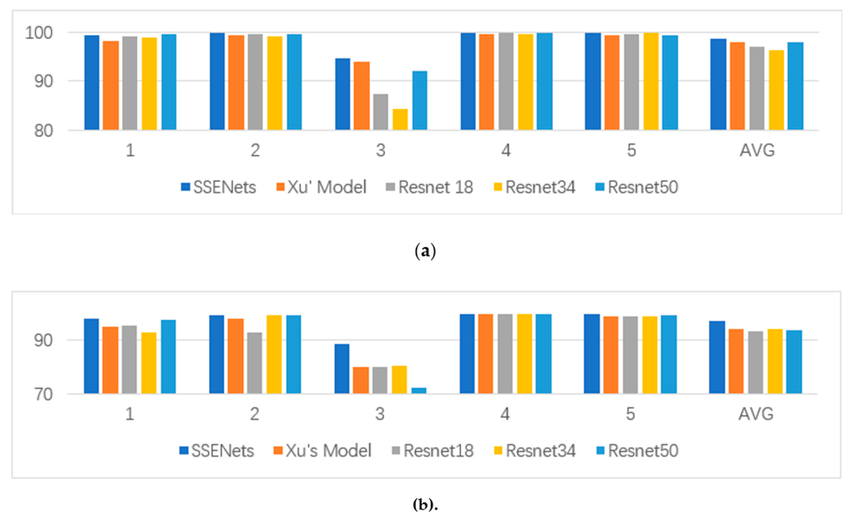
• As shown in Table 8 and Table 9, the testing accuracy has been improved more in comparison to the training accuracy, which shows that SSENets has a better generalization ability. Besides, all the models get low detection accuracy at the third fold cross-validation. The reason is that its testing set contains about two-thirds of the background images, which makes the number of cracks images in training set is far more less than background images. Though this situation will affect the training results of models, SSENets still achieve a higher detection accuracy than other models. Considering the great improvement in the specificity factor, which is shown in Table 7, we conclude that SSENets can reduce the proportion of background images that are classified as crack images.
• Taking advantage of depthwise separable convolution, SSENets has smaller FLOPs and a shorter running time, compared to Resnets. Therefore, SSENets can greatly reduce the complexity of the model and improve the calculation efficiency, thus improving the detection performance of the model.
• Though SSENets could achieve a high detection accuracy in most situations, it still has limitations. As the number of negative samples in the training set decreases, the detection accuracy of SSENets will decrease, so we will devote future work to improving this problem.

4. Conclusions

In this paper, an image classification model SSENets for crack detection is proposed, which is mainly composed of the SSE module using the skip-connection strategy and the ASPP module using the atrous convolution with multi-sample rates. By applying the channel weights generated by shallow feature map to the deeper feature map, SSE module establishes the gradient connection between the shallow network and deeper network. It will alleviate the vanishing gradient during the network training, increase the gradient correlation, and enhance the transmission ability of the model. In view of the crack detection task, we introduce the ASPP module to capture multi-scale features from crack images, thereby improving the accuracy of crack detection. The proposed model can achieve a detection accuracy of 97.77%, which performs better than the comparison models.

Furthermore, the SSE module can be embedded in any convolutional neural network to improve performance. In future work, we will apply SSE module to pixel-level crack detection. Given the computational complexity of this task, we hope that the SSE module will reduce the model parameters while improving the detection accuracy.

References

1. Alipour, M.; Harris, D.K. Increasing the robustness of material-specific deep learning models for crack detection across different materials. Eng. Struct. 2020, 206, 110157. [Google Scholar] [CrossRef]
2. Jahangiri, A.; Rakha, H.A.; Dingus, T.A. Adopting Machine Learning Methods to Predict Red-light Running Violations. In Proceedings of the 2015 IEEE 18th International Conference on Intelligent Transportation Systems, Las Palmas, Spain, 15–18 September 2015; pp. 650–655. [Google Scholar]
3. Jahangiri, A.; Rakha, H.A. Applying Machine Learning Techniques to Transportation Mode Recognition Using Mobile Phone Sensor Data. IEEE Trans. Intell. Transp. Syst. 2015, 16, 2406–2417. [Google Scholar] [CrossRef]
4. Oliveira, H.; Correia, P.L. Automatic Road Crack Segmentation Using Entropy and Image Dynamic Thresholding. In Proceedings of the 2009 17th European Signal Processing Conference, Piscataway, NJ, USA, 24–28 August 2009; pp. 622–626. [Google Scholar]
5. Elbehiery, H.; Hefnawy, A.; Elewa, M. Surface Defects Detection for Ceramic Tiles Using Image Processing and Morphological Techniques. In Proceedings of the WEC’05: 3rd World Enformatika Conference, Istanbul, Turkey, 27–29 April 2005; pp. 158–162. [Google Scholar]
6. Georgieva, K.; Koch, C.; König, M. Wavelet Transform on Multi-GPU for Real-Time Pavement Distress Detection. In Proceedings of the Computing in Civil Engineering 2015. International Workshop on Computing in Civil Engineering, Reston, VA, USA, 21–23 June 2015; American Society of Civil Engineers. pp. 99–106. [Google Scholar]
7. Zhang, A.; Li, Q.J.; Wang, K.C.R. Matched Filtering Algorithm for Pavement Cracking Detection. J. Transp. Res. Rec. 2013, 2367, 30–42. [Google Scholar] [CrossRef]
8. Lecun, Y.; Bottou, L.; Bengio, Y.; Haffner, P. Gradient-based learning applied to document recognition. Proc. IEEE 1998, 86, 2278–2324. [Google Scholar] [CrossRef] [Green Version]
9. Sermanet, P.; Chintala, S.; LeCun, Y. Convolutional Neural Networks Applied to House Numbers Digit Classification. In Proceedings of the 2012 21st International Conference on Pattern Recognition, Univ Tsukuba, Tsukuba, Japan, 11–15 November 2012; pp. 3288–3291. [Google Scholar]
10. He, K.; Zhang, X.; Ren, S.; Sun, J. Deep residual learning for image recognition. In Proceedings of the IEEE Conference on Computer Vision and Pattern Recognition, Boston, MA, USA, 10 December 2015; pp. 770–778. [Google Scholar]
11. Zoph, B.; Vasudevan, V.; Shlens, J.; Le, Q.V.; IEEE. Learning Transferable Architectures for Scalable Image Recognition. In Proceedings of the 2018 Ieee/Cvf Conference on Computer Vision and Pattern Recognition, Salt Lake City, UT, USA, 18–22 June 2018; pp. 8697–8710. [Google Scholar]
12. Zagoruyko, S.; Komodakis, N. Wide residual networks. arXiv 2016, arXiv:1605.07146. [Google Scholar]
13. Redmon, J.; Farhadi, A. YOLO9000: Better, Faster, Stronger. In Proceedings of the 30th IEEE Conference on Computer Vision and Pattern Recognition, Las Vegas, NV, USA, 26 June 2017; pp. 6517–6525. [Google Scholar]
14. Wang, L.; Xiong, Y.; Wang, Z.; Qiao, Y.; Lin, D.; Tang, X.; VanGool, L. Temporal Segment Networks: Towards Good Practices for Deep Action Recognition. In Proceedings of the European Conference on Computer Vision (ECCV), Amsterdam, The Netherlands, 8–16 October 2016; Leibe, B., Matas, J., Sebe, N., Welling, M., Eds.; Springer: Cham, Switzerland, 2016; Volume 9912, pp. 20–36. [Google Scholar]
15. Zhang, A.; Wang, K.C.P.; Li, B. Automated Pixel-Level Pavement Crack Detection on 3D Asphalt Surfaces Using a Deep-Learning Network. J. Comput.-Aided Civil Infrastruct. Eng. 2017, 32, 805–819. [Google Scholar] [CrossRef]
16. Fei, Y.; Wang, K.C.P.; Zhang, A. Pixel-Level Cracking Detection on 3D Asphalt Pavement Images Through Deep-Learning-Based CrackNet-V. IEEE Trans. Intell. Transp. Syst. 2020, 21, 273–284. [Google Scholar] [CrossRef]
17. Song, W.D.; Jia, G.H.; Zhu, H.; Jia, D.; Gao, L. Automated Pavement Crack Damage Detection Using Deep Multiscale Convolutional Features. J. Adv. Transp. 2020, 2020, 1–11. [Google Scholar] [CrossRef]
18. Li, G.; Ma, B.; He, S.; Ren, X.; Liu, Q. Automatic Tunnel Crack Detection Based on U-Net and a Convolutional Neural Network with Alternately Updated Clique. Sensors 2020, 20, 717. [Google Scholar] [CrossRef] [PubMed] [Green Version]
19. Kaseko, M.S.; Ritchie, S.G. A neural network-based methodology for pavement crack detection and classification. Transp. Res. C Emerg. Technol. 1993, 1, 275–291. [Google Scholar] [CrossRef]
20. Chou, J.; Cheng, H.D. Pavement distress classification using neural networks. In Proceedings of the IEEE International Conference on Systems, Man and Cybernetics, New York, NY, USA, 2–5 October 1994; pp. 397–401. [Google Scholar]
21. Nguyen, T.S.; Avila, M.; Begot, S. Automatic detection and classification of defect on road pavement using anisotropy measure. In Proceedings of the 2009 17th European Signal Processing Conference, New York, NY, USA, 24–28 August 2009; pp. 617–621. [Google Scholar]
22. Moussa, G.; Hussain, K. A new technique for automatic detection and parameters estimation of pavement crack. In Proceedings of the 4th Int. MultiConf. Eng. Technol. Innov., Orlando, FL, USA, 19–22 July 2011; pp. 11–16. [Google Scholar]
23. Daniel, A.; Preeja, V. Automatic road distress detection and analysis. Int. J. Comput. Appl. 2014, 101, 18–23. [Google Scholar] [CrossRef]
24. Cha, Y.J.; Choi, W.; Buyukozturk, O. Deep Learning-Based Crack Damage Detection Using Convolutional Neural Networks. Comput. Aided Civil Infrastruct. Eng. 2017, 32, 361–378. [Google Scholar] [CrossRef]
25. Xu, H.; Su, X.; Wang, Y.; Cai, H.; Cui, K.; Chen, X. Automatic Bridge Crack Detection Using a Convolutional Neural Network. Appl. Sci. 2019, 9, 2867. [Google Scholar] [CrossRef] [Green Version]
26. Szegedy, C.; Liu, W.; Jia, Y.; Sermanet, P.; Reed, S.; Anguelov, D.; Erhan, D.; Vanhoucke, V.; Rabinovich, A. Going deeper with convolutions. In Proceedings of the IEEE Conference on Computer Vision and Pattern Recognition, Honolulu, HI, USA, 26 July 2017; pp. 1–9. [Google Scholar]
27. Ioffe, S.; Szegedy, C. Batch normalization: Accelerating deep network training by reducing internal covariate shift. In Proceedings of the International Conference on International Conference on Machine Learning JMLR.org, Lile, France, 6–11 July 2015. [Google Scholar]
28. Szegedy, C.; Vanhoucke, V.; Ioffe, S.; Shlens, J.; Wojna, Z. Rethinking the Inception Architecture for Computer Vision. In Proceedings of the 2016 IEEE Conference on Computer Vision and Pattern Recognition (CVPR), Los Alamitos, CA, USA, 27–30 June 2016. [Google Scholar]
29. Szegedy, C.; Ioffe, S.; Vanhoucke, V.; Alemi, A. Inceptionv4, inception-resnet and the impact of residual connections on learning. In Proceedings of the Thirty-First Aaai Conference on Artificial Intelligence, San Francisco, CA, USA, 4–9 February 2017. [Google Scholar]
30. Chollet, F. Xception: Deep Learning with Depthwise Separable Convolutions. In Proceedings of the 2017 IEEE Conference on Computer Vision and Pattern Recognition (CVPR), Los Alamitos, CA, USA, 21–26 July 2017. [Google Scholar]
31. Howard, A.G.; Zhu, M.; Chen, B.; Kalenichenko, D.; Wang, W.; Weyand, T.; Andreetto, M.; Adam, H. MobileNets: Efficient convolutional neural networks for mobile vision applications. arXiv 2017, arXiv:1704.04861. [Google Scholar]
32. Hu, J.; Shen, L.; Sun, G. Squeeze-and-excitation networks. In Proceedings of the 2018 IEEE/CVF Conference on Computer Vision and Pattern Recognition (CVPR), Los Alamitos, CA, USA, 18–23 June 2018. [Google Scholar]
33. Simonyan, K.; Zisserman, A. Very Deep Convolutional Networks for Large-Scale Image Recognition. In Proceedings of the 3rd International Conference on Learning Representations, ICLR 2015, San Diego, CA, USA, 7–9 May 2015. [Google Scholar]
34. Nair, V.; Hinton, G.E. Rectified Linear Units Improve Restricted Boltzmann Machines Vinod Nair. In Proceedings of the 27th International Conference on Machine Learning (ICML-10), Haifa, Israel, 21–25 June 2010. [Google Scholar]
35. Chen, L.C.; Papandreou, G.; Kokkinos, I.; Murphy, K.; Yuille, A.L. DeepLab: Semantic Image Segmentation with Deep Convolutional Nets, Atrous Convolution, and Fully Connected CRFs. IEEE Trans. Pattern Anal. Mach. Intell. 2018, 40, 834–848. [Google Scholar] [CrossRef] [PubMed]
36. Bridge Crack Detection Based on SSENets. Available online: https://github.com/543630836/Crack_detection_SSENets (accessed on 25 May 2020).
37. Wilson, D.R.; Martinez, T.R. The need for small learning rates on large problems. In Proceedings of the International Joint Conference on Neural Networks, Proceedings (Cat. No. 01CH37222), IJCNN’01, Washington, DC, USA, 15–19 July 2001; pp. 115–119. [Google Scholar]
38. Sokolova, M.; Lapalme, G. A systematic analysis of performance measures for classification tasks. Inf. Process. Manag. 2009, 45, 427–437. [Google Scholar] [CrossRef]
39. Ioffe, S.; Szegedy, C. Batchnormalization: Accelerating deepnetwork training byreducing internal covariate shift. arXiv 2015, arXiv:1502.03167. [Google Scholar]
Figure 1. Flowchart of crack detection.
Applsci 10 04230 g001
Figure 2. Illustration of the crack detection network, SSENets.
Applsci 10 04230 g002
Figure 3. Structure of Skip-Squeeze-Excitation (SSE) Module.
Applsci 10 04230 g003
Figure 4. Simplified model of SSE module.
Applsci 10 04230 g004
Figure 5. Structure of Atrous Spatial Pyramid Pooling (ASPP) Module.
Applsci 10 04230 g005
Figure 6. Histograms of 5-fold cross-validation. (a) The detection accuracy of training; (b) The detection accuracy of testing.
Applsci 10 04230 g006