Article

Exploring Benefits of Using Blending Splines as Transition Curves

Faculty of Engineering Science and Technology, UiT The Arctic University of Norway, Lodve Langesgate 2, 8514 Narvik, Norway
*
Author to whom correspondence should be addressed.
Appl. Sci. 2020, 10(12), 4226; https://doi.org/10.3390/app10124226
Submission received: 19 May 2020 / Revised: 15 June 2020 / Accepted: 16 June 2020 / Published: 19 June 2020

Abstract

:
Track geometry is a fundamental subject in railway construction. With the demand for increased capacity in terms of load and speed, the need for suitable transitions between consecutive track sections is highly relevant. Properly constructed transition curves lead to improved travel comfort, increased safety, and reduced wear. The well known clothoid curve is widely used as a transition curve; however, the linear curvature is not sufficiently smooth to meet the requirements for railways carrying high speed trains or heavy hauls. Blending spline curves are flexible spline constructions possessing favourable smoothness properties at the end points, which makes them considerable for use as transition curves. This paper demonstrates some selected blending splines applied as transition curves between two existing circular arc segments selected from the Ofotbanen railway. The main results in this paper are related to the smoothness at the end points and the behaviour of the curvature of the curves, where the new transition curves were shown to be smoother than the original clothoid. Another new result is the observation that the proposed method allows for the improvement of existing railways without forcing extensive changes to the original track. Some representative examples are included to highlight the flexibility of this first instance of blending splines as transition curves.

1. Introduction

Transition curves are an important development in the railway industry. They were introduced to create easements between straight and curved railway sections, and between curved sections of different radii. Properly constructed transition curves increased safety and comfort while travelling, and reduced wear on the rail [1,2]. Various curves have been recommended as transition curves over the years, among them, the clothoid [3,4], which has become the most used to this day. The search for new types of transition curves for railways is still relevant and ongoing, due to new knowledge related to curve properties [5], where the linear curvature of the clothoid is not smooth enough in the end regions to be optimal. Both in relation to passenger comfort, for speeds above 120 km/h [6], and in relation to wear on the tracks with heavy haul traffic.
The recent research on transition curves can be divided into linear- and non-linear curvature curves. The most common topic of the two is non-linear curvature curves, since the problem of increasing curvature smoothness has received attention. Some examples are a remodelling of the cubic parabola [7], a new design of the Bloss curve [8], sinusoid transition curves [9], and the Wiener Bogen curves [10]. Under the topic of linear curvature curves, two types of curves have been analysed: log-aesthetic curves [6], which are identified to give equal properties as clothoids, and Symmetrically Projected Transition Curves [11], which are simpler and more accurate curves compared to the clothoid and cubic parabolas, and are meant as a better option in cases where the cubic parabola is preferred over the clothoid.
In addition, experiments have been performed on hybrid solutions, e.g., curves with linear middle parts and non-linear ends. Two examples are parametric transition curves [12] and smoothed transition curves [13,14]. All of the previously mentioned curves are curves that replace a single element in the railway. However, there is also research where multiple elements are replaced. General transition curves [15,16] and universal transition curves [17,18] are curves that replace the segments: first transition curves–circular arc–second transition curve, or first transition curves–second transition curve. Multiple element transition curves are not investigated in this paper, but are interesting for future work.
A common denominator with the research on transition curves is that there is rarely a connection between research and industry, as can be observed in [19]. A challenge here is replacing segments in an already existing railway. Recent research does not take into account the layout of the new transition curves and the effects they will have on the existing railway, in regard to the horizontal alignment of the rail.
A blending spline curve [20] is a spline construction where local functions are blended together by C k -smooth blending functions. Blending splines were introduced [21] as an additional tool in computer-aided geometric design (CAGD) with emphasis on user interactivity via the editing capabilities. Due to the flexibility in the blending process, when connected to possible local functions and blending functions, the authors suggest that the spline may be suitable as a transition curve.
The scope of this study was to find a new railway transition curve, with better properties than the clothoid in regard to the smoothness between segments, that can replace the clothoid in an already existing railway without making changes to the original alignment. The need to be able to increase smoothness without making extensive changes to the alignment is relevant for existing railways where large modifications may be invasive or impossible. One example is Ofotbanen, a Norwegian railway line, essential in the transportation of ore from Kiruna in Sweden, and goods between the northern and southern parts of Norway [22]. Ofotbanen is known for its challenging railway geometry, which is vulnerable to wear. Making extensive changes to the alignment of Ofotbanen requires considerable intervention and is impossible in some places due to the mountainous terrain the railway ventures through.
The aim of the study was to reveal the suitability of blending splines as a transition curve, replacing one segment (a clothoid) in an already existing railway. A focus was given to making the least amount of intervention to the existing railway by considering the segments attached to the clothoid static, and only allowing the length of the transition curve to increase by moving the entry points along the adjacent segments. In this paper, blending splines of various forms were implemented and analysed as transitions between two circular arc segments of dissimilar radii. The new transition curves were compared to the replaced clothoid by analysing their curvature functions against each other, and drawing conclusions based on the smoothness and value of the curvature derivatives. This is the first time blending splines have been considered as transition curves, and, to the best of the authors’ knowledge, the first time adjacent railway segments remained fixed.
The remainder of the paper is organised as follows: Section 2 gives a short explanation of blending splines and transition curves. In Section 3, the methods are described. Section 4 presents the obtained results, together with a discussion on the data. Lastly, Section 5 draws a conclusion and gives recommendations for future work.

2. Preliminaries

The preliminaries section provides an overview of the relevant theory connected to the work. A short presentation of the blending spline is given, together with a brief overview of transition curves in railway.

2.1. Blending Spline

A blending spline is a collective term of the family of blending-type spline constructions originating from research conducted since 2003. The initial blending spline, called Expo-rational B-spline (ERBS), was presented for the first time in [23] and within two years published in [20,24]. After that the family grew, with new splines derived from the ERBS, including generalized expo-rational B-splines [25] and logistic expo-rational B-splines [26]. The blending spline is a construction where local functions at the knots are blended together by C k -smooth basis functions, see Figure 1. It is defined in [21] as
f ( t ) = k = 1 n l k ( t ) B k ( t ) , t ( t 1 , t n ] ,
where the coefficients l k ( t ) are scalar-, vector-, or point-valued local functions defined on ( t k 1 , t k + 1 ) . t = { t k } k = 0 n + 1 is an increasing knot vector, and B k ( t ) are the blending functions (B-functions). The B-functions can be any function possessing the following set of properties:
  • B : I I ( I = [ 0 , 1 ] R ) ,
  • B ( 0 ) = 0 ,
  • B ( 1 ) = 1 ,
  • B ( t ) 0 , t I ,
  • B ( t ) + B ( 1 t ) = 1 , t I .
The last property is optional and specifies the point symmetry around the point ( 0.5 , 0.5 ) . Figure 2 shows a plot of possible B-functions meeting the properties. In this paper, we considered a subset of ERBS called the scalable subset, proposed in [21], that used a specific B-function (the ERB-function), which is C -smooth,
B k ( t ) = S k 1 0 ω k 1 ( t ) ψ k 1 ( s ) d s if t k 1 < t t k , S k ω k ( t ) 1 ψ k ( s ) d s if t k < t < t k + 1 , 0 otherwise ,
where S k = ( 0 1 ψ ( s ) d s ) 1 , ω k ( t ) = t t k t k + 1 t k , and ψ k ( s ) = e β | s λ | α ( 1 + γ ) ( s ( 1 s ) γ ) α with the intrinsic parameters restricted to α > 0 , β > 0 , γ > 0 , and 0 λ 1 . We also note that the ERBS shares the minimal support and partition of unity properties of the linear B-spline, which means that only two functions are blended together in every knot interval (i.e., between two knots) and that the two B-functions in the interval sum up to 1 for a given t. By applying the two previous properties, the simplified formula of (1), over one knot interval, becomes
f ( t ) = B k ( t ) l k ( t ) + B k + 1 ( t ) l k + 1 ( t ) = ( 1 B k + 1 ( t ) ) l k ( t ) + B k + 1 ( t ) l k + 1 ( t ) = l k ( t ) + B k + 1 ( t ) ( l k + 1 ( t ) l k ( t ) ) .
For the experiments in this paper, we use parametric curves as local functions l k ( t ) . The specific choices are presented and explained in Section 3.2.

2.2. Transition Curves

In railway design, the transition curves fulfill the role of connecting straight sections to curved sections, and curved sections of different radii [27]. The task of the transition curve is to gradually decrease/increase the radius of the curvature from radius R 1 to R 2 , and to provide a change in superelevation following the same behaviour as the curvature, usually by linear, Bloss, sine, or cosine functions. These properties are important in order to counteract a sudden jerk in the centrifugal forces, and instead gently introduce them over the course of the transition curve. The main advantages of using transition curves are [28,29]:
  • Providing a comfortable ride for passengers.
  • Providing a safer ride for passengers.
  • Enabling the vehicle to drive at a higher speed.
  • Reducing the wear and tear on wheels and rails, thus, decreasing the maintenance and repair costs.
As mentioned in the introduction, the clothoid is the most used transition curve today. One of the first discoveries of the clothoid as a transition curve in railways was by Arthur Talbot in [30], who was among the first to approach the transition problem mathematically. A clothoid (of length l and end radius r) is a spiral defined parametrically as
x y = C ( t ) S ( t ) ,
where C ( t ) and S ( t ) are the Fresnel integrals,
C ( t ) = 1 a 0 t ^ cos π 2 u 2 d u , S ( t ) = 1 a 0 t ^ sin π 2 u 2 d u ,
with a = 1 π r l being a scaling factor, and t ^ = a t , < t < . A main reason for the clothoid’s popularity as a transition curve is its curvature, which changes linearly with the curve length.

3. Method

This section describes the parameters and equations used in setting up the original (existing) railway curve example, the relevant parameters for creating the blending spline transition curve and how they are modified, and an explanation of the criteria for comparing the blending spline against the clothoid from the original railway track.

3.1. The Original Railway Curve

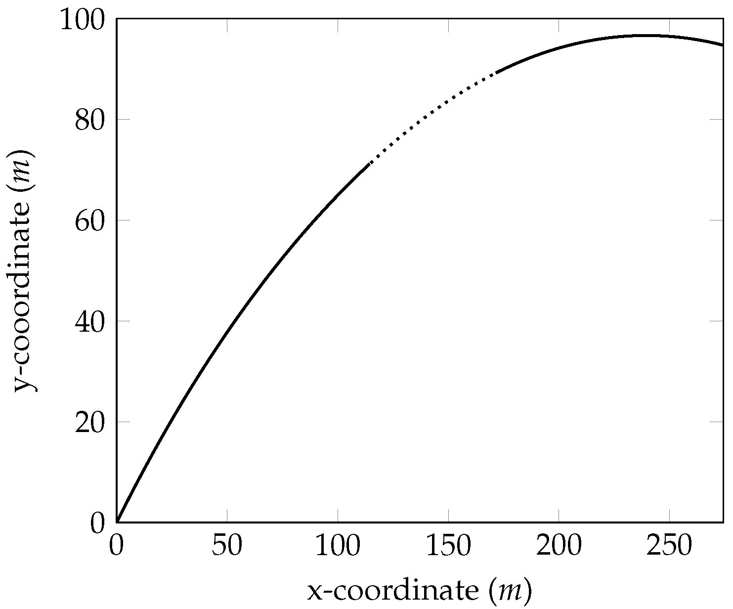
The original railway curve consists of two arc segments, of different radii, connected by a clothoid transition curve. The example is extracted from the Norwegian railway line, Ofotbanen. Parameters for the segment are presented in Table 1, with the layout plotted in Figure 3.
The clothoid is implemented by exploiting a power series expansion of the integrals in (5), given in [31] as,
C ( t ) = 1 a i = 0 ( 1 ) i ( π 2 ) 2 i t ^ 4 i + 1 ( 2 i ) ! ( 4 i + 1 ) , S ( t ) = 1 a i = 0 ( 1 ) i ( π 2 ) 2 i + 1 t ^ 4 i + 3 ( 2 i + 1 ) ! ( 4 i + 3 ) ,
where the variable a is set up for the clothoid to join two arcs, instead of an arc and a line.

3.2. Blending Spline Fitting

The blending spline curve is created for one knot interval, using expression (3), in order to preserve the maximum flexibility over the entire transition curve. It is relevant to adjust three parameters in this study: entry points, local curves, and B-functions.

3.2.1. Entry Points

The entry points for the blending spline on the adjacent circular segments were tested for three positions: [ p 1 , q 1 ] , [ p 2 , q 2 ] , and [ p 3 , q 3 ] , as shown in Figure 4. [ p 1 , q 1 ] is the same entry point as the clothoid, [ p 2 , q 2 ] is placed 1 4 of the circular segment’s curve length from [ p 1 , q 1 ] , and [ p 3 , q 3 ] is in the middle of the circular segment. The motivation for choosing entry points only on half of the circular segments is to account for the possibility of also creating blending splines on both sides of the example segments, so that future work can include the replacement of multiple clothoid segments.

3.2.2. Local Curves

The curves that can be used as local curves in a blending spline transition curve have to comply with three criteria. They must have the correct curvature for one end, be possible to connect to adjacent segments with a smoothness equal to or higher than the clothoid, and be scalable in length. The most intuitive curves to use as local curves in the blending spline, for this transition case, are circular arc segments, given by
c ( t ) = ( R sin ( t ) , R ( 1 cos ( t ) ) ) , 0 < t < 2 π ,
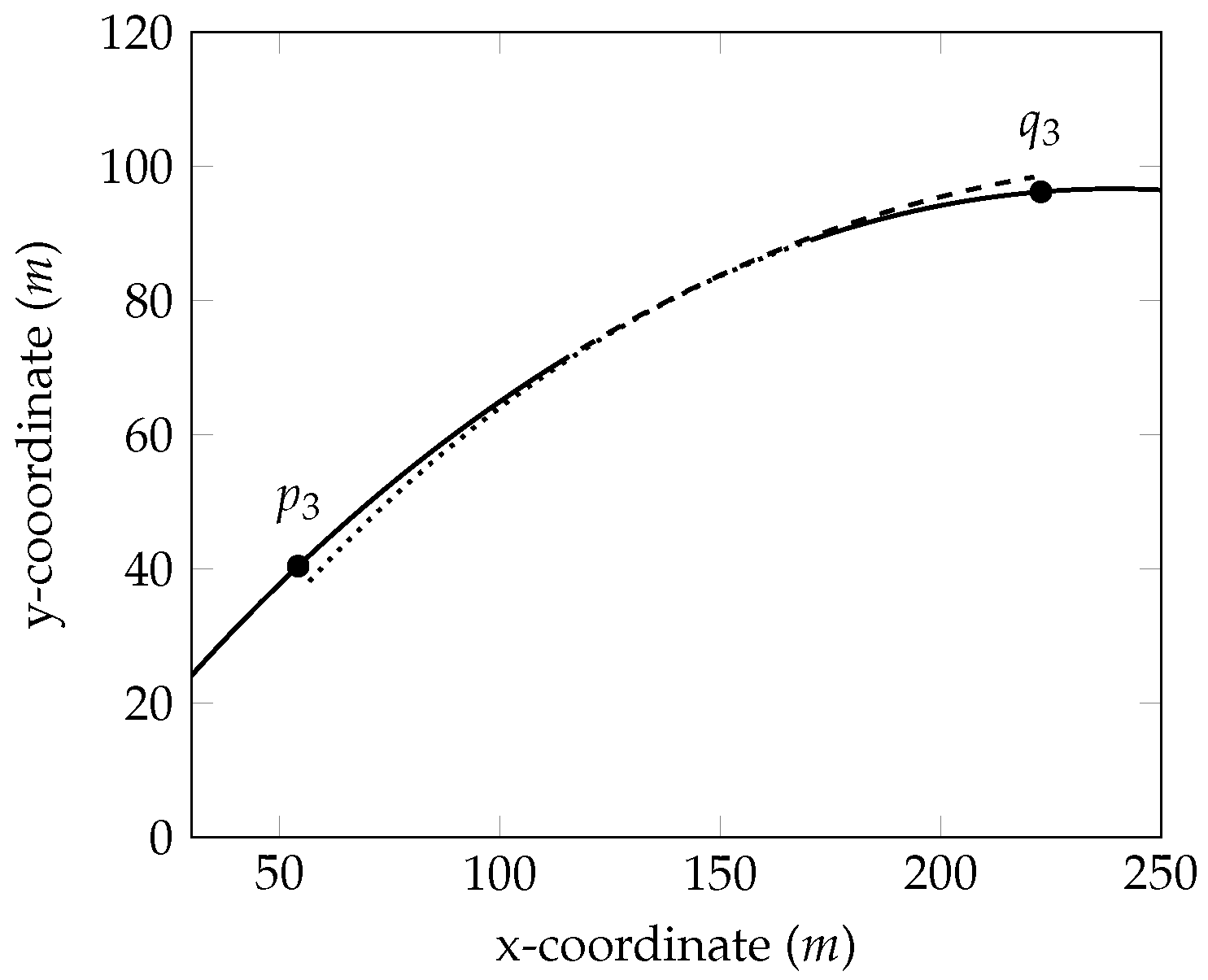
with the same radius R as the original railway arcs (401 and 315, in this case). They have the correct curvature and smoothness for at least one end, are easy to scale in size, and easy to place correctly against the adjacent segments. An example of two local arc curves starting at entry point [ p 3 , q 3 ] is shown in Figure 5.
In addition to the circular arcs, Bézier curves are also tested as local curves in the blending spline. Bézier curves are industry standard representations of free-form shapes, and are available in most design and CAD software. They are expressed as
c ( t ) = i = 0 n c i b i , n ( t ) ,
where c i are control points, and b i , n ( t ) are Bernstein polynomials of degree n. Compared to the arcs, the Bézier curves are more flexible as their shapes can be altered through control points. The Bézier curves in this research are created by approximating the previously described arcs via performing a Taylor expansion of a point and d derivatives in the entry points (which becomes the start of the Bézier curves). To achieve sufficient smoothness at the entry points, while also having the opportunity to manipulate the control point at the opposite end, the degree of the Bézier curves should be at least four ( d > 3 ). For the local Bézier curve examples in this paper, the number of derivatives extracted in the start point is 4, which means that d = 4 and 5 control points are placed.
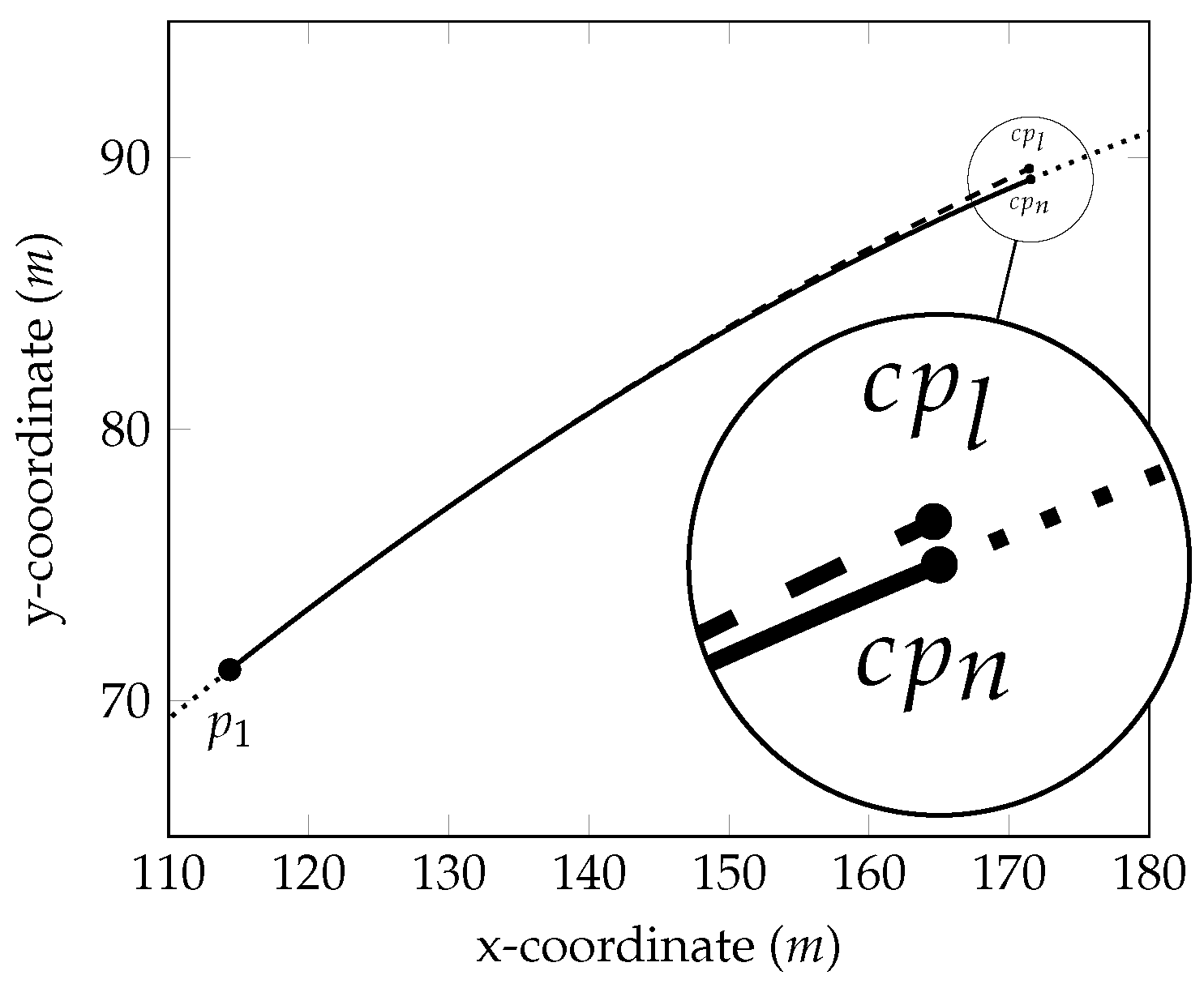
To maintain a smooth connection to the adjacent circular arc segments, while at the same time experimenting with the placement of the local curves, the first four control points, from the start of the curves, are fixed and the last control point is moved to the start of the local curve in the opposite end. A visual explanation is given in Figure 6. This is expected to give different results compared with using arcs as local curves, and to show if placing the local curves closer to the original clothoid has a significant effect on the curvature.

3.2.3. B-Function

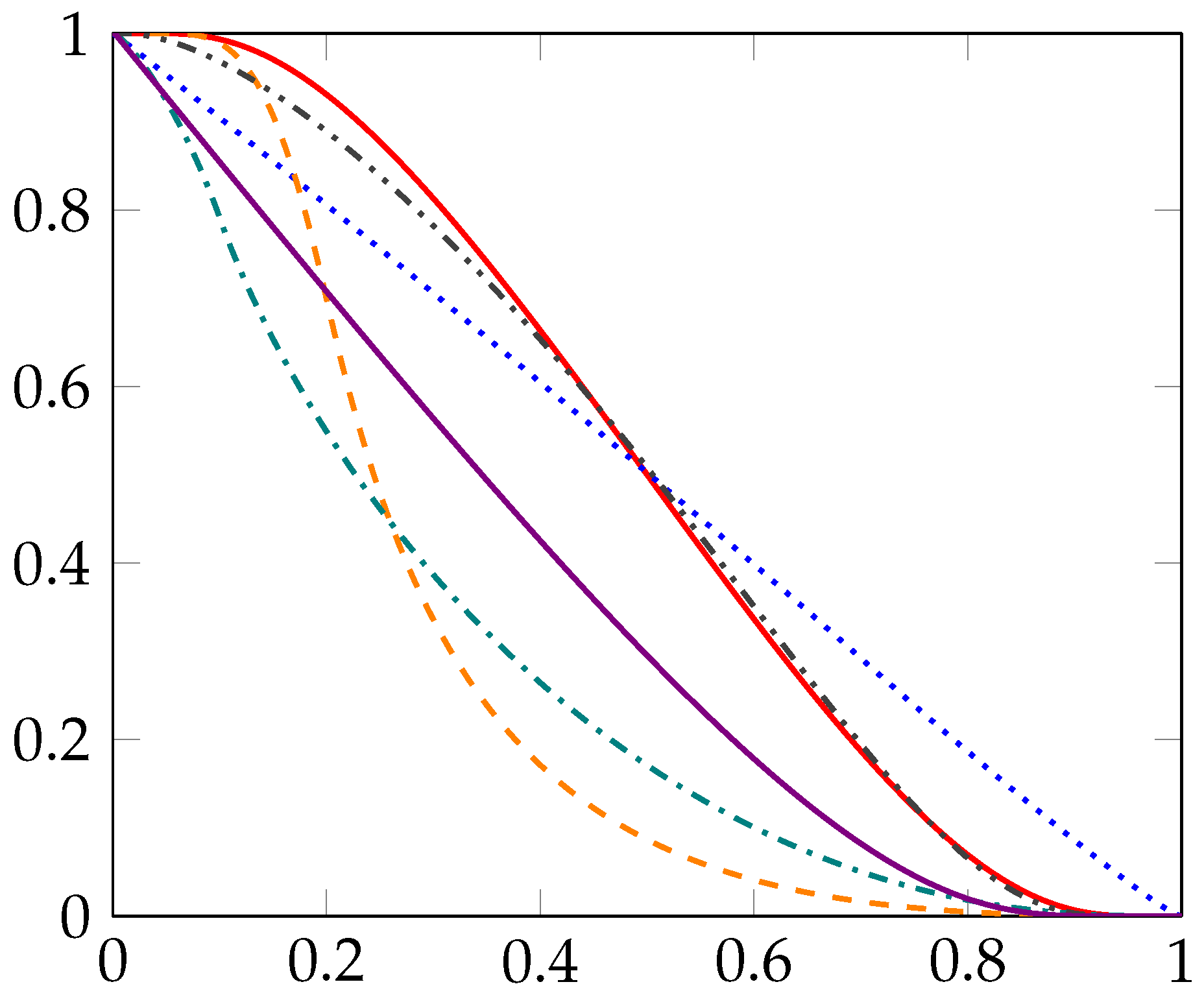
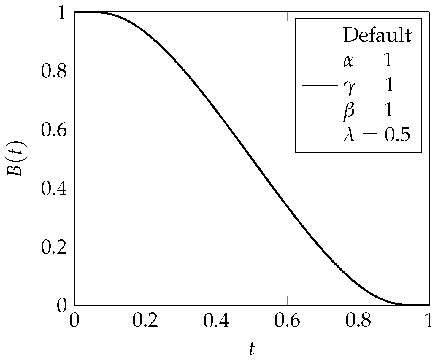
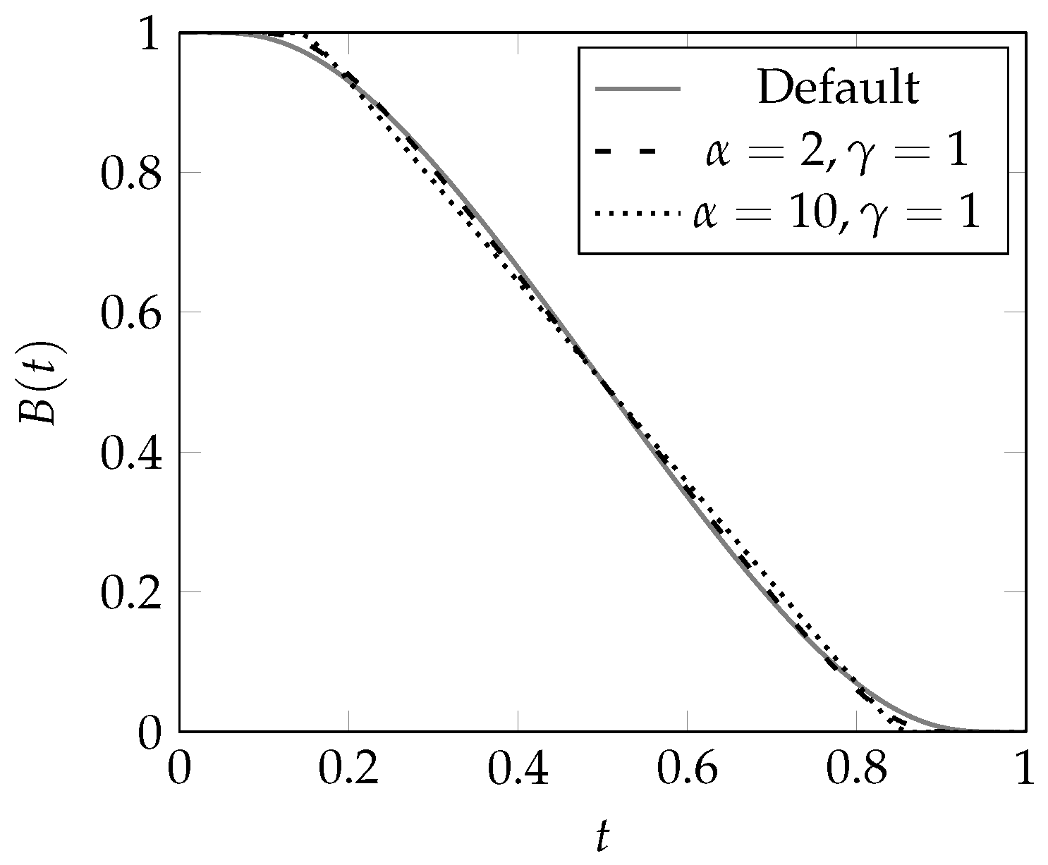
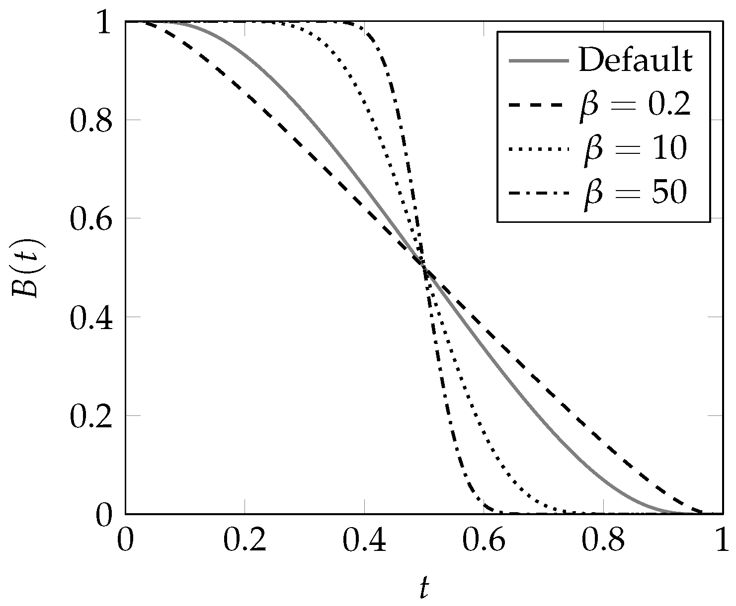
The B-funtion used in the study is the one presented in (2), an ERB-function. This function can be varied through the following parameters: α > 0 , β > 0 , γ > 0 , and 0 λ 1 , where α , γ N and β , λ R . The default ERB-function is given by α = 1 , β = 1.0 , γ = 1 , and λ = 0.5 , as seen in Figure 7. α and γ are called the asymmetric tightening parameters. Increasing them tightens the function so that its shape goes toward a linear function on parts of the domain. Figure 8 shows plots of ERB-functions with varying tightening values. β is called the slope parameter. This adjusts the steepness of the function.
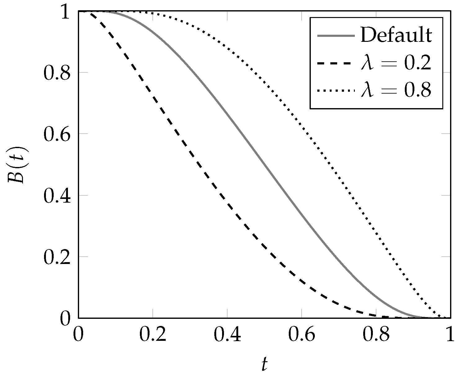
Figure 9 shows ERB-functions with varying slope values. λ is called the balance parameter. Varying this moves the function along the x-axis. Figure 10 gives plots of ERB-functions with varying balance values. For the comparisons in this paper, the parameters were adjusted independently, modifying one while keeping the default values for the rest. The tested values for each parameter are given in Table 2. They are selected based on the shape differences that they bring to the B-function, so that a range of contrasting blending functions are tested.

3.3. Comparison Criteria

To evaluate the blending spline as a transition curve it was compared against the original clothoid with the following criteria, presented in [6].
  • Common connection point: the coordinates of the two curves must be equal in the connection points.
  • Common tangent: the tangents of the two curves must be equal in the connection points.
  • Equal radius of curvature: the radii of the two curves must be equal in the connection points (eliminates discontinuities in the form of jumps in the curvature diagram).
  • Common tangent of curvature functions: the first derivative of the curvature functions of the two curves must be equal in the connection points (eliminates discontinuities in the form of breaks in the curvature diagram).
  • Equal radius of curvature of curvature functions: the second derivative of the curvature functions of the two curves must be equal in the connection points (needed for extremely high-speed railways).
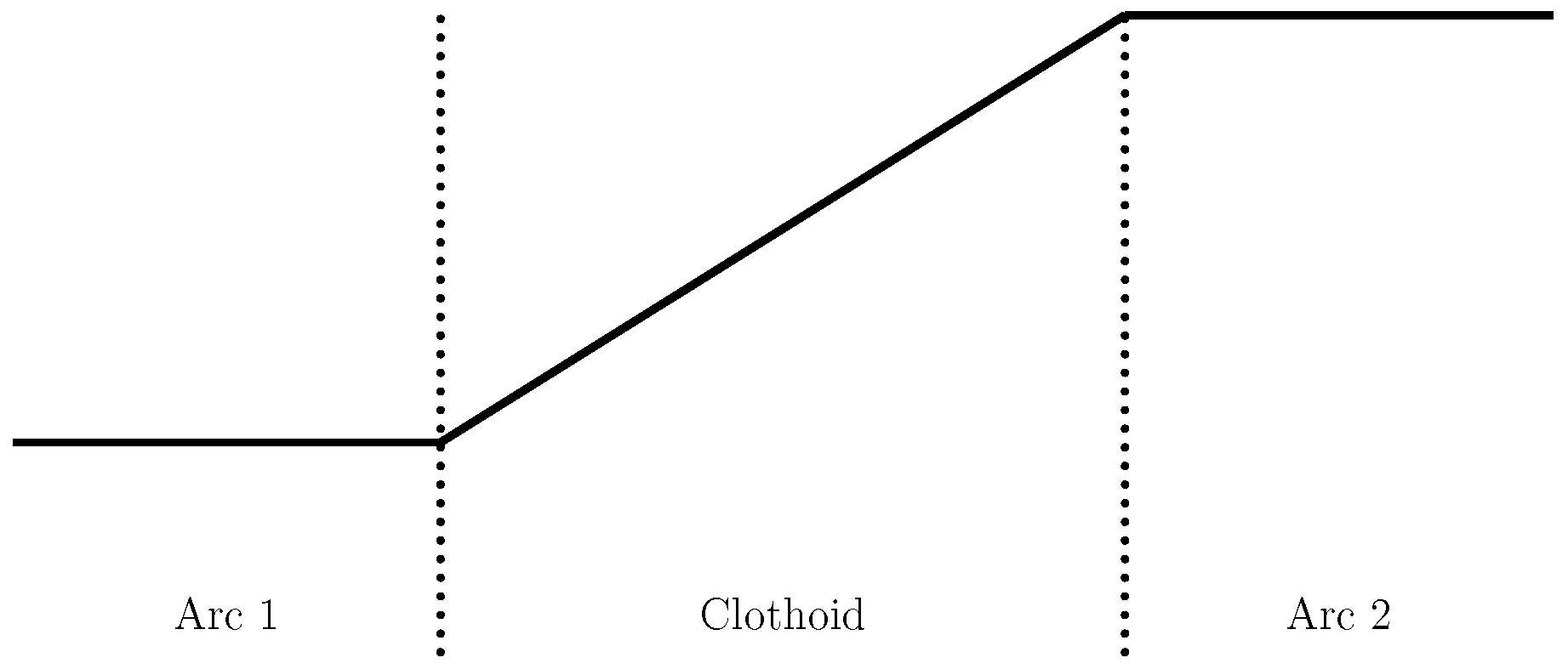
The clothoid fulfills criterion 1 to 3, which means that it has discontinuities in the form of breaks in the curvature diagram, see Figure 11. The reason for considering only the curvature, as an evaluation criteria, is the close connection it has to the jerk of the railway wagon, for instance through Lateral change of acceleration (LCA) [5].

3.4. Experimental Set-Up

The experiments were conducted via computer programming utilizing the in-house software library GMlib [32,33]. Geometric descriptions of the existing railway were implemented with GMlib to provide a reference for comparison of the new results with the original data. All curves were implemented as parametric curves and the data were extracted by evaluating the curves uniformly from start to end. The curve properties that were of interest in this paper were the curvature, and the first and second derivative of the curvature. These properties were analysed and compared by visual examination of the graphs plotted from the evaluated data, and the focus was on the behaviour of the graphs and values at the end points. Comparisons were made between the curvatures of the existing railway segments and the blending splines, and in addition, the curvatures of the various blending splines were compared against each other.

4. Results and Discussions

This section shows the results of the method applied to the Ofotbanen example described in Section 3.1. The results are divided in two, based on the type of local curves used in the blending spline: arcs and Béziers. For each of the local curves, the curvature plots of the blending splines were analysed and discussed, and compared with the clothoid, for varying entry points and ERB-function parameters. The curvature is presented as κ in the figures, and κ -der represents the first and second derivatives of the curvature.

4.1. Arc as Local Curves

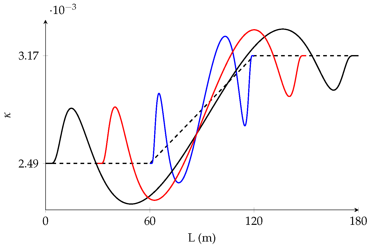
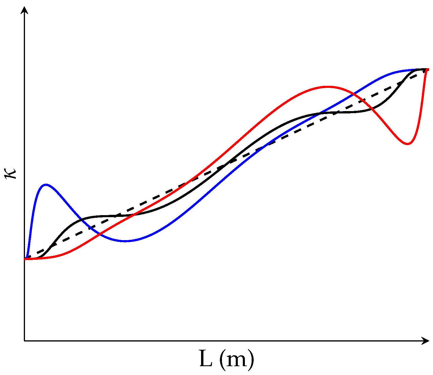
Curvature plots for the clothoid and three blending spline transition curves (with entry points [ p 1 , q 1 ] , [ p 2 , q 2 ] , and [ p 3 , q 3 ] ), using circular arcs as local curves and a default ERB-function for blending, can be seen in Figure 12. The dashed function is the clothoid curvature, while the solid functions are blending spline curvatures ( [ p 1 , q 1 ] in blue, [ p 2 , q 2 ] in red, and [ p 3 , q 3 ] in black). From the figure, it can be seen that changing the entry points did not have a great impact on the behaviour of the blending spline. The main difference was the length of the curves ( L = 60 m for [ p 1 , q 1 ] , L = 120 m for [ p 2 , q 2 ] , and L = 180 m for [ p 3 , q 3 ] ), which arose from the selection of entry points.
Compared to the clothoid’s linear curvature, the blending splines have five inflection points in their curvature graphs, which is not optimal and should be attempted smoothed out. A positive characteristic of the blending splines is that they go smoothly towards the end points, where the clothoid has a discontinuity in connection to the constant curvature of the adjacent segments, as described in Figure 11. This leads us to believe that the blending spline, at least with a default ERB-function, satisfies the additional criteria (4 and 5 presented in Section 3.3) when compared to the clothoid.
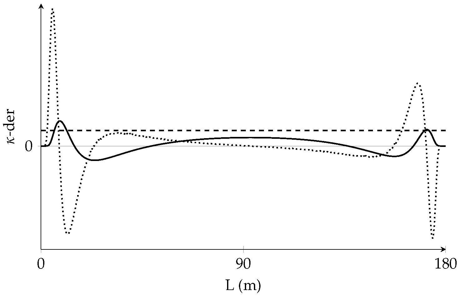
To test our hypothesis, graphs of the first and second derivatives of the curvature for the blending spline in [ p 3 , q 3 ] were printed. As the behaviour was fairly familiar for the three blending splines in the end points only one was checked. The result can be seen in Figure 13, where the constant first derivative of the clothoid’s curvature (dashed) is plotted against the first (solid) and second (dotted) derivatives of the blending spline’s curvature. From the figure, it can be observed that the first and second derivatives of the blending spline go to zero in the ends. These conditions are exactly what is needed to fulfill criteria 4 and 5. Hence, the blending spline is better than the clothoid when it comes to smoothness in the connection points to the adjacent segments.
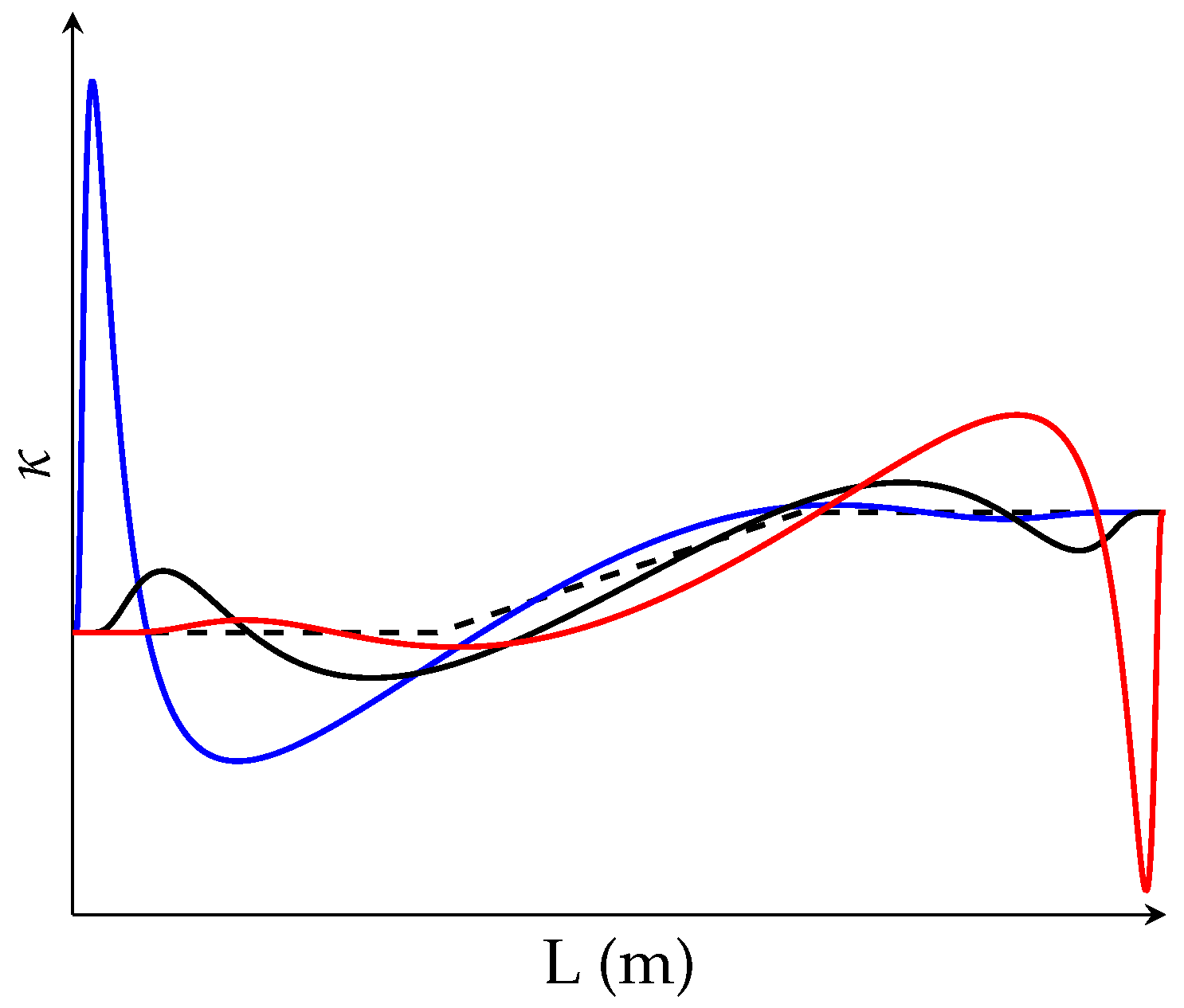
From the previous results, an assumption can be made that any blending spline with a smoother curvature diagram towards the end points, than the default ERB-funtion blending spline, will meet all the criteria in Section 3.3. Thus, the focus of the discussion when varying the ERB parameters will be on smoothing the curvature along the blending spline. In the adjustment of the ERB parameters, the curves that are studied have entry points [ p 3 , q 3 ] .
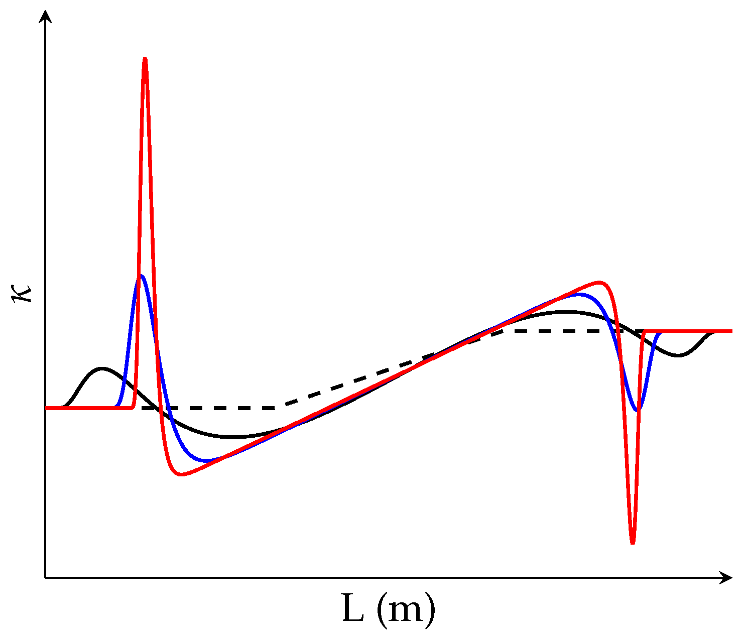
By varying the tightening parameters, α and γ , as described in Table 2, the resulting curvature diagrams, of the blending splines, become as shown in Figure 14. From the plots, it can be observed that by increasing α , the smoothness in the end points increased and the bumps became more prominent, with higher amplitudes of the extreme values. By varying the slope parameter, β , as described in Table 2, the resulting curvature diagrams, of the blending splines, became as plotted in Figure 15. From the plots, it can be observed that by increasing β , the bumps were shifted toward the middle of the graph and the smoothness increased in the end points. By varying the balance parameter, λ , as described in Table 2, the resulting curvature diagrams, of the blending splines, became as plotted in Figure 16. From the plots, it can be observed that by moving the balance of the ERB-function left or right, the smoothness increased in one end and decreased in the other. The same was true for the bumps: in one end they were smoothed, while in the other they became more prominent.
Attempting to smooth the curvature by varying the ERB parameters was not straightforward. It seems that the slope parameter can dampen the fluctuations to some extent, which was also the case in one end when varying the balance parameter. However, overall, the ERB parameters did not change the characteristics of the curvature, they only affected the extreme values and shifted the amplitude of the bumps.

4.2. Bézier as Local Curves

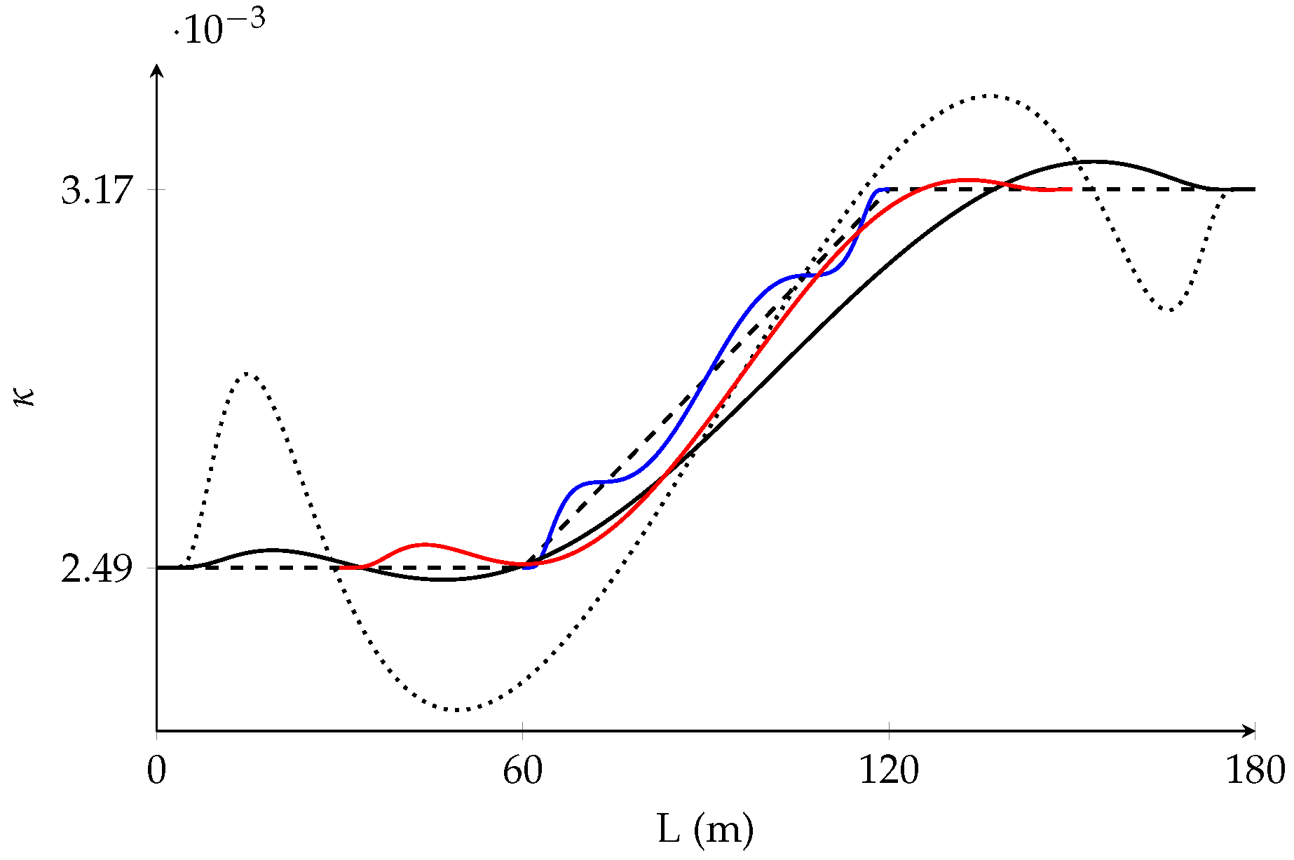
Using Bézier curves as local curves and starting with a default ERB-function for blending, the curvature for the three blending spline transition curves together with the clothoid, and the blending spline in [ p 3 , q 3 ] from Figure 12, can be seen in Figure 17. As before, the dashed function is the clothoid curvature, while the solid functions are blending spline curvatures. In addition, a blending spline (dotted) with local arc curves in [ p 3 , q 3 ] was plotted for comparison. From the figure, it can be seen that using Bézier curves as local curves, instead of arcs, yielded blending splines with curvatures that lay closer to the clothoid, while still having a smooth transition to the end points. With this observation, we concluded that the three first criteria from Section 3.3 were fulfilled, and that there is a possibility that more criteria are met.
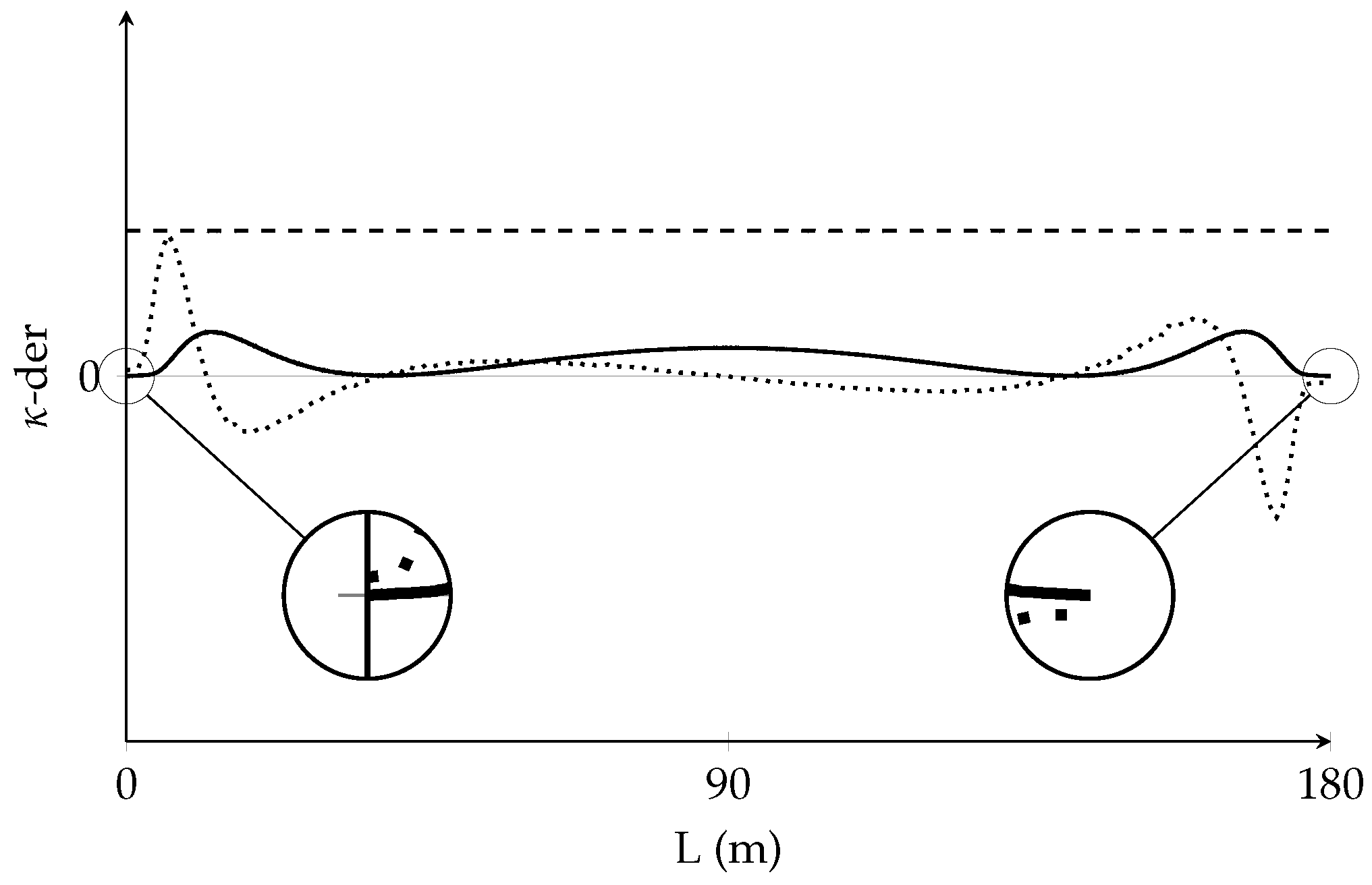
In Figure 18 the first (solid) and second (dotted) derivative of the curvature for the blending spline in [ p 1 , q 1 ] are plotted, together with the first derivative of the curvature for the clothoid (dashed). From the figure, it can be observed that the first derivative of the blending spline went to zero in the ends, while the second derivative ended a little above and below zero in the two end points. This indicates that criterion 4 was fulfilled, but not criterion 5, as there will be a small jump in the connection points for the second derivative function. However, the blending spline with local Bézier curves was still better than the clothoid for smoothness in the connection points to the adjacent segments. One method of increasing the smoothness, so that it also fulfills criterion 5, could be to raise the degree of the Bézier curves from d = 4 to d = 5 , and fix the first four control points.
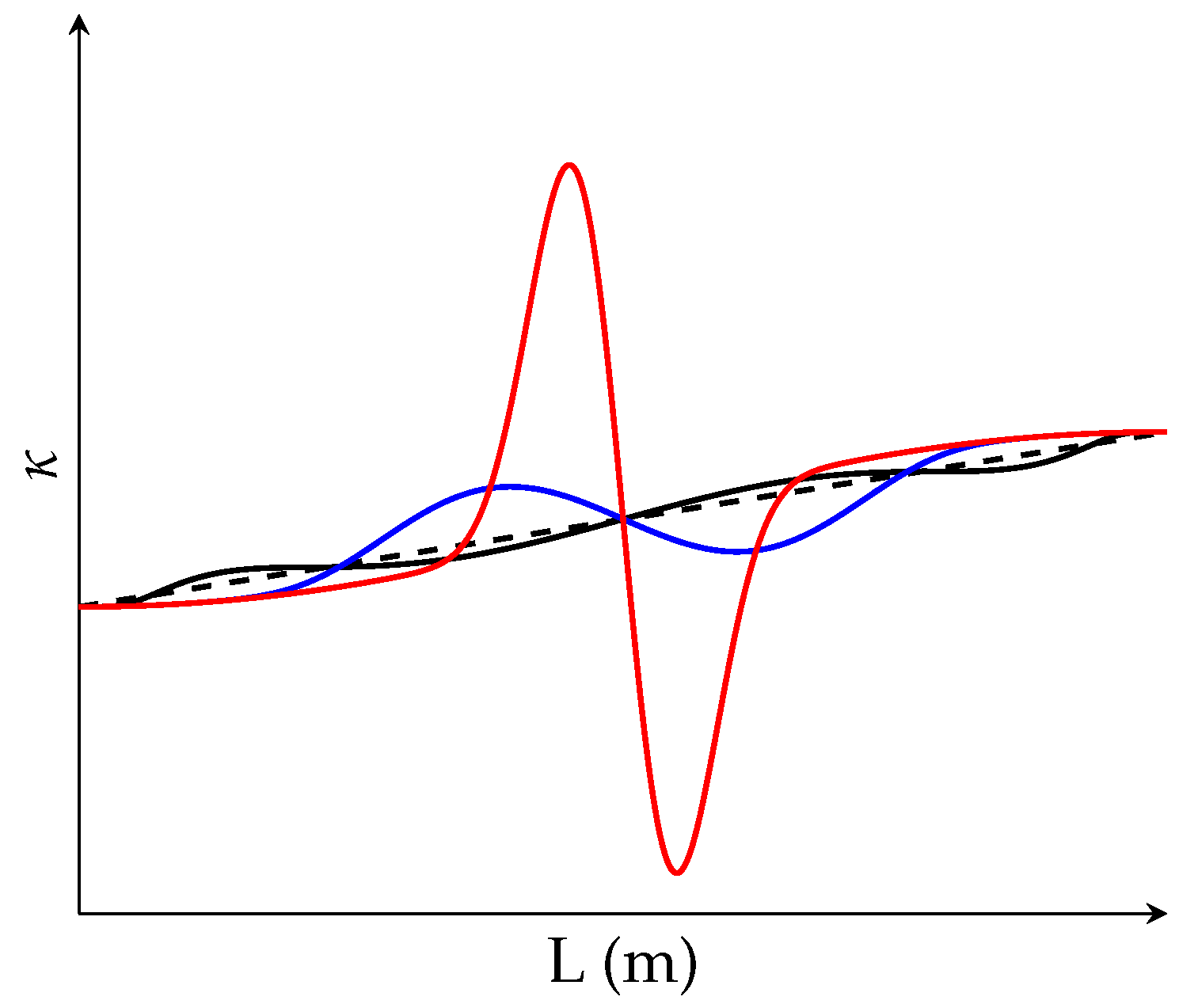
The same assumption is made here, as in the discussion with arc curves, that any blending spline with a smoother curvature diagram towards the end points, than the default ERB-function blending spline, will fulfill criteria 1–4 in Section 3.3. Thus, the focus when varying the ERB parameters will be on smoothing the curvature along the blending spline. In the variation of the ERB parameters, the curves that were studied had entry points [ p 1 , q 1 ] , because the curvature lay closest to the clothoid in Figure 17. The parameters were varied in the same manner as with the blending spline with local arc curves, described in Table 2. In Figure 19, the tightening parameters were varied; in Figure 20, the slope parameter was varied; and in Figure 21, the balance parameter was varied.
The results that emerged were very similar to the results obtained for the blending spline with local arc curves: by varying the tightening parameters, the smoothness in the end points increased and the bumps became more prominent, with higher extreme values. By varying the slope parameters, the bumps were shifted toward the middle and the smoothness increased in the ends. By varying the balance parameter, the smoothness increased in one end and decreased in the other, and the bumps were smoothed in one end, while becoming more prominent in the other.
Thus, with these results, a conclusion can be drawn, that the ERB parameters did not change the behaviour of the curvature, they only affected the extreme values and shifted the amplitude of the bumps. However, a new result was obtained here, showing that by re-shaping the local curves, the characteristics of the curvature can be changed, causing smaller fluctuations along the function.

5. Concluding Remarks

In this paper, a family of splines (blending splines) were applied and analysed as transition curves for an already existing railway. Three segments from the Ofotbanen railway were extracted as two circular arcs connected by a clothoid. The goal was to make the least amount of intervention to the existing railway, by keeping the placement of the arcs unchanged and only allowing the transition curve entry points to move. Under this constraint, the blending splines were compared to the clothoid with regard to the smoothness of the end points and the shape of the curvature graph. The main findings in the paper can be summarized as follows:
  • the blending spline transition curves had a higher degree of curvature smoothness ( G 1 ) in the connection points compared to the clothoid, which was G 0 ;
  • the blending spline yielded the possibility of replacing transition curves in an existing railway without moving the adjacent segments;
  • the choice of blending function and local curves had a large impact on the curvature of the curve, and on the degree of smoothness in the connection points.
The results showed that the blending splines, with appropriately selected local curves, were smoother than the clothoid for the ends. However, the curvature plots of the blending splines had fluctuations along the lengths, which may not be optimal in a transition case if the fluctuations are large. An observation was made that the choice of ERB parameters and local curves had a large impact on these fluctuations. The choice of local curve type and shape had an even larger impact. By using Bézier curves as local curves, with a default ERB-function, the fluctuations were relatively small, as can be observed in Figure 17. The curvature function was close to a monotonically increasing function, which seems to be the norm for transition curves. However, there exists at least one transition curve that is not, the Wiener Bogen [10].
The Wiener Bogen uses a non-monotonically increasing curvature curve together with a monotonically increasing superelevation ramp, which provides better transition properties than the clothoid. Whether the blending spline curves can be used in the same manner as the Wiener Bogen remains to be tested, and may yield interesting results if the blending splines are smoother in the end points when compared with the clothoid. A different approach, which is very relevant for future work, is to test other local curves that may dampen the fluctuations more (or even remove them). From the results on local Bézier curves, it will be of interest to raise the degree of the Bézier so that more than one control point in the ends can be manipulated. There are strong indications that these extra degrees of freedom can be utilized to smooth the curvature function more than for fourth degree Bézier curves where only one control point is manipulated.
In this work, the control point was moved manually in order to test the hypothesis. However, there are indications that it would be possible to develop an algorithmic solution for the placement of the control points in the local Bézier curves, under the constraints of a given optimal curvature. This, together with inspecting ERB-functions where several parameters are modified, with respect to the characteristics of the resulting curvature, is out of scope in the current paper and is considered for future work.
From a technical point of view, the local curves of the proposed transition curves can be represented in already existing software, as circular arcs and Bézier curves are fundamental elements in CAD. Utilizing blending spline transition curves with established workflows and software tools can then be performed in several ways. For example, the blending spline evaluator can be implemented as a stand alone tool (requiring export, processing, and import of the data), as a plug in, or integrated into an existing software package.
The new transition curves were developed from a geometric point of view. The analysis was conducted by utilizing pure geometric comparison criteria, as outlined in Section 3.3. The maintenance and modification of existing railways provides certain additional challenges. As pointed out in [34], one would have to consider additional mechanical parameters, such as the wheel–rail conditions, to deal with track cant transitions. Kaewunruen et al. [35,36] demonstrated that wheel–rail contact forces relate to the curvature distribution, and that rail surface defects, or squats, commonly appear along the transition arc length [36,37]. The smoothness of the spline construction yields extra derivatives, which may assist track cant transition design. For this reason, it would be interesting to investigate the performance of practical blending spline transition curves with respect to the relation between track geometry and wheel–rail interface problems; however, it would be important to optimize the curvature fluctuations to avoid disadvantageous rail squat development.

Author Contributions

Conceptualization, T.F.B. and R.D.; software, T.F.B.; formal analysis, T.F.B.; investigation, T.F.B.; resources, T.F.B.; data curation, T.F.B.; writing—original draft preparation, T.F.B.; writing—review and editing, T.F.B. and R.D.; visualization, T.F.B.; supervision, R.D. All authors have read and agreed to the published version of the manuscript.

Funding

The publication charges for this article were funded by a grant from the publication fund of UiT The Arctic University of Norway.

Conflicts of Interest

The authors declare no conflict of interest.

References

  1. Glover, J. Transition curves for railways. Proc. Inst. Civ. Eng. 1900, 140, 161–179. [Google Scholar]
  2. Miller, A.W. The transition spiral. Aust. Surv. 1939, 7, 518–526. [Google Scholar] [CrossRef]
  3. Archibald, R.C. Euler Integrals and Euler’s Spiral, Sometimes Called Fresnel Integrals and the Clothoide or Cornu’s Spiral. Am. Math. Mon. 1918, 25, 276–282. [Google Scholar]
  4. Higgins, A.L. The Transition Spiral and Its Introduction to Railway Curves With Field Exercises in Construction and Alignment; Van Nostrand Company: New York, NY, USA, 1922. [Google Scholar]
  5. Baykal, O. Concept of Lateral Change of Acceleration. J. Surv. Eng. 1996, 122, 132–141. [Google Scholar] [CrossRef]
  6. Arslan, A.; Tari, E.; Ziatdinov, R.; Nabiyev, R. Transition Curve Modeling with Kinematical Properties: Research on Log-Aesthetic Curves. Comput. Aided Des. Appl. 2014, 11, 509–517. [Google Scholar] [CrossRef] [Green Version]
  7. Shebl, S. Geometrical analysis of non-linear curvature transition curves of high speed railways. Asian J. Curr. Eng. Math. 2016, 5, 52–58. [Google Scholar] [CrossRef]
  8. Ciobanu, C. Bloss transition—A short design guide. PWI J. 2015, 133, 14–18. [Google Scholar]
  9. Pirti, A.; Yücel, M.; Ocalan, T. Transrapid and the transition curve as sinusoid. Tehnički Vjesnik 2016, 23, 315–320. [Google Scholar]
  10. Wojtczak, R. Charakterystyka Krzywej Przejściowej Wiener Bogen®; Publishing House of Poznan University of Technology: Poznan, Poland, 2017. [Google Scholar]
  11. Eliou, N.; Kaliabetsos, G. A new, simple and accurate transition curve type, for use in road and railway alignment design. Eur. Transp. Res. Rev. 2014, 6, 171–179. [Google Scholar] [CrossRef] [Green Version]
  12. Koc, W. Transition Curve with Smoothed Curvature at its Ends for Railway Roads. Curr. J. Appl. Sci. Technol. 2017, 22, 1–10. [Google Scholar] [CrossRef]
  13. Koc, W. Smoothed transition curve for railways. Przeglad Komunikacyjny 2019, 19–32. [Google Scholar] [CrossRef]
  14. Koc, W. New Transition Curve Adapted to Railway Operational Requirements. J. Surv. Eng. 2019, 145. [Google Scholar] [CrossRef]
  15. Kobryn, A. Use of polynomial transition curves in the design of horizontal arcs. Roads Bridges Drogi i Mosty 2017, 16, 5–14. [Google Scholar]
  16. Kobryn, A. New Solutions for General Transition Curves. J. Surv. Eng. 2014, 140, 12–21. [Google Scholar] [CrossRef]
  17. Kobryn, A. Universal Solutions of Transition Curves. J. Surv. Eng. 2016, 142, 04016010. [Google Scholar] [CrossRef]
  18. Kobryn, A.; Stachera, P. S-Shaped Transition Curves as an Element of Reverse Curves in Road Design. Baltic J. Road Bridge Eng. 2019, 14, 484–503. [Google Scholar] [CrossRef]
  19. Brustad, T.F.; Dalmo, R. Railway Transition Curves: A Review of the State-of-the-Art and Future Research. Infrastructures 2020, 5, 43. [Google Scholar] [CrossRef]
  20. Dechevsky, L.T.; Lakså, A.; Bang, B. Expo-rational B-splines. Int. J. Pure Appl. Math. 2006, 27, 319–369. [Google Scholar]
  21. Lakså, A. Basic properties of Expo-Rational B-splines and practical use in Computer Aided Geometric Design. Ph.D. thesis, University of Oslo, Oslo, Norway, 2007. [Google Scholar]
  22. Bane Nor. Ofotbanen. Available online: https://www.banenor.no/jernbanen/banene/ofotbanen/ (accessed on 3 July 2019).
  23. Dechevsky, L.T. Expo-rational B-splines. In Proceedings of the Sixth International Conference on Mathematical Methods for Curves and Surfaces, Tromsø, Norway, 1–6 July 2004. [Google Scholar]
  24. Dechevsky, L.T.; Lakså, A.; Bang, B. Exploring Expo-Rational B-splines for Curves and Surfaces. In Mathematical Methods for Curves and Surfaces; Dæhlen, M., Mørken, K., Schumaker, L.L., Eds.; Nashboro Press: Brentwood, TN, USA, 2005; pp. 253–262. [Google Scholar]
  25. Dechevsky, L.T.; Bang, B.; Lakså, A. Generalized expo-rational B-splines. Int. J. Pure Appl. Math. 2009, 57, 833–872. [Google Scholar]
  26. Dechevsky, L.T.; Zanaty, P. Smooth GERBS, orthogonal systems and energy minimization. AIP Conf. Proc. 2013, 1570, 135–162. [Google Scholar]
  27. Mundrey, J. Railway Track Engineering, 4th ed.; Tata McGraw-Hill: New York, NY, USA, 1988. [Google Scholar]
  28. Hickerson, T.F. Route Location And Design, 5th ed.; McGraw-Hill: New York, NY, USA, 1964. [Google Scholar]
  29. Lipičnik, M. New Form of Road/Railway Transition Curve. J. Transp. Eng. 1998, 124, 546–556. [Google Scholar] [CrossRef]
  30. Talbot, A. The Railway Transition Spiral; Reprinted from The Technograph No. 13; University Illinois: Champaign, IL, USA, 1899. [Google Scholar]
  31. Abramowitz, M.; Stegun, I.A. Handbook of Mathematical Functions With Formulas, Graphs, and Mathematical Tables; Dover Publications, Inc.: New York, NY, USA, 1972. [Google Scholar]
  32. Lakså, A.; Bang, B.; Kristoffersen, A.R. GM_lib, a C++ Library for Geometric Modeling; Technical report; Narvik University College: Narvik, Norway, 2006. [Google Scholar]
  33. UiT The Arctic University of Norway. GMlib/GMlib2 C++ Geometric Modeling Library. 2019. Available online: https://source.coderefinery.org/gmlib (accessed on 3 June 2020).
  34. Chrostowski, P.; Koc, W.; Palikowska, K.; Kaewunruen, S. Discussion: Prospects in elongation of railway transition curves. Proc. Inst. Civ. Eng. Transp. 2018. [Google Scholar] [CrossRef] [Green Version]
  35. Kaewunruen, S.; Ishida, M.; Marich, S. Dynamic Wheel–Rail Interaction Over Rail Squat Defects. Acoust. Aust. 2015, 43, 97–107. [Google Scholar] [CrossRef]
  36. Kaewunruen, S.; Ishida, M. In Situ Monitoring of Rail Squats in Three Dimensions Using Ultrasonic Technique. Exp. Tech. 2016, 40, 1179–1185. [Google Scholar] [CrossRef]
  37. Wilson, A.; Kerr, M.; Marich, S.; Kaewunruen, S. Wheel/rail conditions and squat development on moderately curved tracks. In Proceedings of the Rail—The Core of Integrated Transport: CORE 2012: Conference On Railway Engineering, Brisbane, Australia, 10–12 September 2012; pp. 223–230. [Google Scholar]
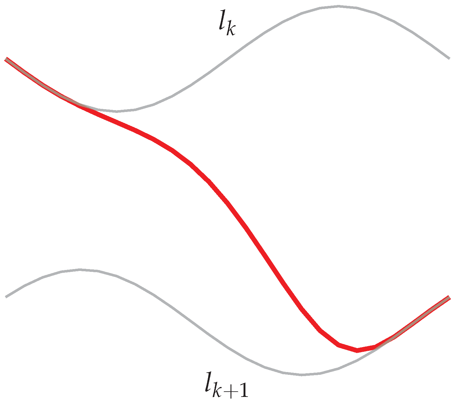
Figure 1. Two local curves ( l k and l k + 1 ) blended together to create a blending spline (red curve).
Applsci 10 04226 g001
Figure 2. Plots of possible blending functions.
Applsci 10 04226 g002
Figure 3. Layout of the original railway curve. Two circular arc segments (solid) connected by a clothoid segment (dotted).
Applsci 10 04226 g003
Figure 4. The three entry points for the blending spline transition curve on the circular segments.
Applsci 10 04226 g004
Figure 5. An example of two local arc curves (dashed and dotted) starting in [ p 3 , q 3 ] .
Applsci 10 04226 g005
Figure 6. An example of how the last control point c p l is moved to the start of the local curve in the opposite end c p n , for the left side local Bézier curve starting in p 1 . The dashed curve is the first Bézier approximation of the arc, and the solid curve is the one used in the blending.
Applsci 10 04226 g006
Figure 7. Plot of the default ERB-function.
Applsci 10 04226 g007
Figure 8. Plots of Expo-rational blending functions (ERB-functions) with varying tightening parameters. The solid function is the default ERB ( α = γ = 1 ), the dashed function has α = 2 and γ = 1 , and the dotted function has α = 10 and γ = 1 .
Applsci 10 04226 g008
Figure 9. Plots of ERB-functions with varying slope parameters. The solid function is the default ERB ( β = 1 ), the dashed function has β = 0.2 , the dotted function has β = 10 , and the dashdotted function has β = 50 .
Applsci 10 04226 g009
Figure 10. Plots of ERB-functions with varying balance parameters. The solid function is the default ERB ( λ = 0.5 ), the dashed function has λ = 0.2 , and the dotted function has λ = 0.8 .
Applsci 10 04226 g010
Figure 11. Curvature diagram of a clothoid connected to two arc segments of different radii.
Applsci 10 04226 g011
Figure 12. Curvature plots of the clothoid with parts of the circular segments (dashed) and default ERB-function blending splines, with local arc curves, for the three entry points [ p 1 , q 1 ] (blue), [ p 2 , q 2 ] (red), and [ p 3 , q 3 ] (black).
Applsci 10 04226 g012
Figure 13. Plots of the first derivative of the curvature for the clothoid (dashed) and default ERB-function blending splines, with local arc curves, in [ p 3 , q 3 ] (solid), and the second derivative of the curvature for the blending spline, scaled by 1 10 (dotted).
Applsci 10 04226 g013
Figure 14. Curvature plots of the clothoid with parts of the circular segments (dashed) and blending splines in [ p 3 , q 3 ] for tightening parameters α , γ = 1 , 1 (black, default), α , γ = 4 , 1 (blue), and α , γ = 10 , 1 (red).
Applsci 10 04226 g014
Figure 15. Curvature plots of the clothoid with parts of the circular segments (dashed) and blending splines in [ p 3 , q 3 ] for slope parameters β = 1.0 (black, default), β = 8.0 (blue), and β = 50.0 (red).
Applsci 10 04226 g015
Figure 16. Curvature plots of the clothoid with parts of the circular segments (dashed) and blending splines in [ p 3 , q 3 ] for balance parameters λ = 0.5 (black, default), λ = 0.2 (blue), and λ = 0.8 (red).
Applsci 10 04226 g016
Figure 17. Curvature plots of the clothoid with parts of the circular segments (dashed) and default ERB-function blending splines, with local Bézier curves, for the three entry points [ p 1 , q 1 ] (blue), [ p 2 , q 2 ] (red), and [ p 3 , q 3 ] (black). In addition, the curvature of a blending spline with local arc curves, in [ p 3 , q 3 ] , is plotted (dotted).
Applsci 10 04226 g017
Figure 18. Plots of the first derivative of the curvature for the clothoid (dashed) and default ERB-function blending splines, with local Bézier curves, in [ p 1 , q 1 ] (solid), and the second derivative of the curvature for the blending spline, scaled by 1/10 (dotted).
Applsci 10 04226 g018
Figure 19. Curvature plots of the clothoid (dashed) and blending splines in [ p 1 , q 1 ] for tightening parameters α , γ = 1 , 1 (black, default), α , γ = 4 , 1 (blue), and α , γ = 10 , 1 (red).
Applsci 10 04226 g019
Figure 20. Curvature plots of the clothoid (dashed) and blending splines in [ p 1 , q 1 ] for slope parameters β = 1.0 (black, default), β = 8.0 (blue), and β = 50.0 (red).
Applsci 10 04226 g020
Figure 21. Curvature plots of the clothoid (dashed) and blending splines in [ p 1 , q 1 ] for balance parameters λ = 0.5 (black, default), λ = 0.2 (blue), and λ = 0.8 (red).
Applsci 10 04226 g021
Table 1. Segment parameters.
Arc 1ClothoidArc 2
Start Radius (m)-401315
End Radius (m)401315-
Length (m)135.33560103.481
Table 2. Expo-rational blending function (ERB-function) parameter values used in the comparisons.
α γ β λ
Default111.00.5
Tightening 1411.00.5
Tightening 21011.00.5
Slope 1118.00.5
Slope 21150.00.5
Balance 1111.00.2
Balance 2111.00.8