Understanding Digital Radio Frequency Memory Performance in Countermeasure Design

Abstract

This paper describes the design, implementation, and testing of a novel multi-function software defined Radio Frequency (RF) system designed for small airborne drone applications. The system was created using an inexpensive Field Programmable Gate Array (FPGA) to combine a coherent linear frequency modulated radar transmitter and receiver, with a Digital Radio Frequency Memory (DRFM) jammer for use with a common RF aperture in simultaneous operation. The system was implemented on a Xilinx Kintex-7 FPGA with a wideband analogue-to-digital/ digital-to-analogue (ADC/DAC) converter mezzanine board and tested using hardware-in-the-loop mode to validate its performance. This is the first known account of an integrated multifunction electronic attack and radar system on a single chip, capable of performing a simultaneous, not time shared, operation.

1. Introduction

Digital Radio Frequency Memory (DRFM) jammers have existed for several decades now, evolving from simple mono-bit devices to modern wideband, high dynamic range systems, with fully coherent receivers and transmitters [1]. Despite this, no published research has been conducted to understand the fundamental relationship of a DRFM system: the interaction between the deceptive waveform it generates and the radar receiver [2,3,4,5,6,7,8,9,10]. Understanding of the DRFM-radar interaction is fundamental to Electronic Attack (EA) design, allowing for the proper jammer waveform parameters (power, frequency, technique, etc.) to be chosen for maximum effectiveness. The goal of this paper is to illuminate that relationship, the factors that affect it, and propose a more effective DRFM architecture in order to improve the Electronic Attack (EA) and Electronic Protection (EP) engineering processes.

The results of this study quantify the processing loss, time delay, and side-lobe levels generated in a variety of scenarios, providing guidance in the design of effective EA. Building on the study of DRFM jammer-radar receiver interaction, a novel jammer architecture is proposed and implemented to effectively counter modern forms of electronic protection.

Prior to recent years, one of the limitations of studying the jammer-radar interaction was the available hardware. National agencies were often limited to their in-service jammers, or radars, many of which had limited signal agility to validate experimental results. Fortunately, Field Programmable Gate Arrays (FPGA) and the related tools, such as MATLAB, Simulink and Xilinx System Generator, allow for the generation of software defined EW and radar systems, with all aspects of the digital implementation being under the engineer’s control. This research exploited FPGA technology to implement a wide variety of waveforms, and DRFM jammer architectures using a Xilinx Kintex-7 FPGA, in order to evaluate the factors that affect EA/EP performance.

To do so, a wideband DRFM was implemented in two forms, a fully-coherent in-phase and quadrature (I-Q) sampling DRFM, and an envelope DRFM that only sampled the amplitude. This approach is a reflection of the two classes of DRFM jammer available and allowed the various effects that degraded the jammer performance to be examined in both architectures. The remainder of this paper describes the DRFM research in detail, by providing background on DRFM jammers and their performance, detailing the DRFM model developed, and the performance during the various experiments.

Finally, the problem of DRFM systems generating signals in response to radars capable of modern forms of EP, which require the generation of signals emulating a multiple scatterer target, is explored. Specifically, a novel DRFM architecture is proposed and implemented on an FPGA that demonstrates the ability to emulate EA from a multiple scatterer target.

2. DRFM Systems

At the fundamental level, DRFM systems are a transceiver capable of digitizing, recording to memory, modifying, and re-transmitting the recorded waveform. Doing so requires a variety of sub-systems: receivers, Analogue-to-Digital Converters (ADC), Digital Signal Processing (DSP), Electronic Attack (EA) control system, Digital-to-Analogue Converters (DAC), and transmitters [11,12,13,14]. This section discusses these various sub-systems, the associated distortions that occur when recording and re-transmitting a waveform, and the use of software defined EW systems to implement a DRFM. The intent is to provide the background necessary to understand how the DRFM systems were modeled and implemented digitally.

DRFM systems have been in existence since the 1980s [15], with two themes driving their advance: digitizer performance, and a move to software defined systems. The first EW receivers were largely driven by single bit or mono-bit ADCs as the bandwidths required allowed for very restricted resolution with the existing technology [16] (this literally means the ADC had only a single bit for measuring amplitude, making the automatic gain control systems critical to the jammer performance).

ADC and DAC performance is not the restricting factor anymore, as devices operating above at multiple giga-samples per second with 10 or more bits of resolution are common [17]. Instead, the bottleneck is the throughput of the resulting bit streams, especially in multi-channels commonly seen in direction finding.

The other trend, software defined radios, is what allows for this research to occur, as previously, DRFMs could be modeled, or hardware implementations could be built at great expense. Now Field Programmable Gate Arrays (FPGA), and the associated model level tools, such as Xilinx System Generator or Lab View, allow for the creation of software defined EW systems in days, with a much narrower set of engineering skills.

2.1. Digital Radio Frequency Memory

The digital equivalent of a tape recorder for radar signals, DRFM systems are generally composed of the following parts: receiver, transmitter, signal processing, digital memory, and the ECM control system. While the antenna and/or array can vary in design significantly, the remainder of the RF front-end is generally a variation of the super-heterodyne receiver [18]. The range of frequencies covered, with the high end being 18 to 40 GHz in radar jammers, requires an external up-conversion and down conversion stage. The frequency translation from IF to baseband is usually performed digitally in modern systems [19].

Once on the FPGA, the detection and Pulse Descriptor Word (PDW) encoder determine the presence of a signal and encode a PDW. Depending on the signal detected, this could trigger a recording to the DRFM. At this point, the ECM control system takes over, generating an ECM based on the recorder waveform by adjusting the time delay and Doppler shift before re-transmitting.

2.2. Sources of Distortion

Nothing in the previous section is unusual from the design of an RF transceiver for a radar or communications system, the difference with a DRFM is the wide bandwidth of the receiver, which significantly exceeds the signal and the requirement to repeat the signal, instead of demodulating it for a radio or performing detection in a radar. This presents a problem, as the signal replicated by the jammer has been distorted at every stage of the reception and retransmission process.

The factors that could affect its accuracy in recreating the received waveform and that will be studied in this chapter include the thermal noise, quantization noise, the type of DRFM (amplitude or in-phase/quadrature), and the modulation of the waveform itself. While outside the scope of this paper, the RF front-end would also create non-linear effects, particularly while re-transmitting the signal at high power.

To replicate a modern DRFM, a Field Programmable Gate Array (FPGA) implementation was performed. This FPGA implementation not only simplifies the development, it largely mirrors the modern jammer architecture, as the cost of the development cost of Application Specific Integrated Circuits (ASIC) has driven EW systems to increasingly capable FPGAs [6]. The second benefit is it allowed the system not to be modeled but to actually be implemented on the device, and to do so in numerous iterations quickly. The flexible nature of a software defined EW system on an FPGA, effectively means the factors affecting DRFM performance were tested against actual jammers, implemented digitally, with only the RF front-end modeled.

3. DRFM System Model

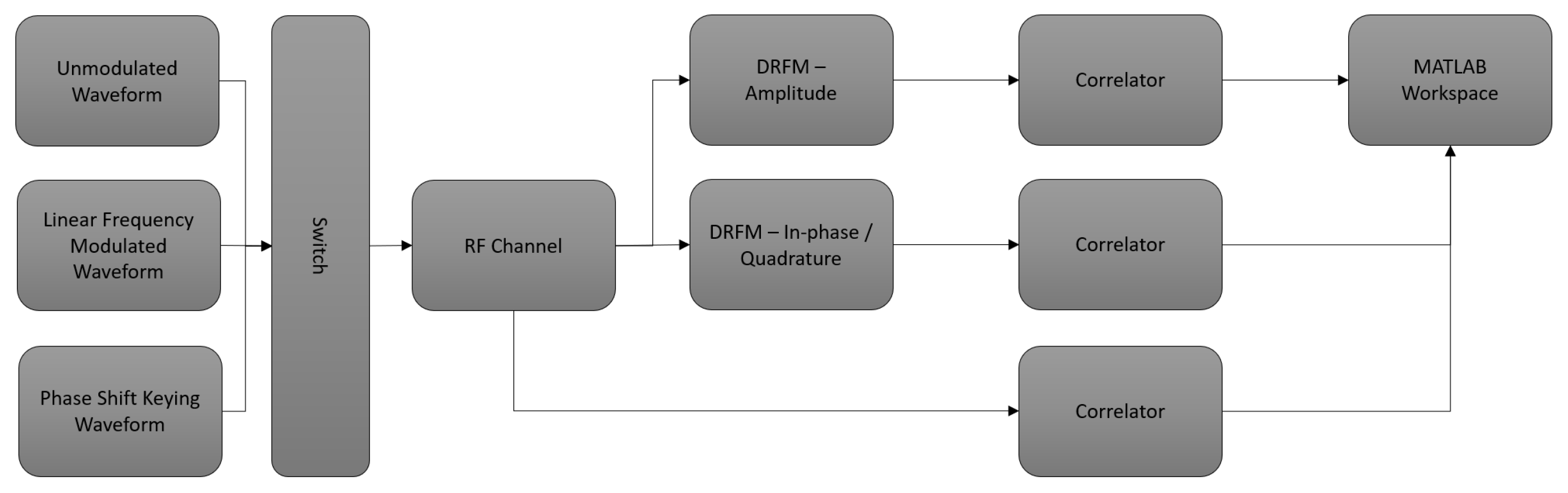
The DRFM system was implemented in three parts, as shown in Figure 1, forming the MATLAB testbed and FPGA DRFM implementation: the radar signal sources, the DRFM jammer, and the correlator bank. The system, described in detail in this section, generated radar signals in the testbed, sent them through the DRFM jammer for retransmission and used the correlator to compare the received signals to the transmitted signal in a variety of cases.

A correlator was used to measure how the jammer waveform and transmitted waveform resembled each other. The output of the correlators was then sent to MATLAB as arrays of samples in the time domain for plotting and analysis; this is discussed in the next section.

3.1. Radar Transmitter

The radar transmitter implementation, shown in Figure 2, is capable of generating three classes of radar signals that cover most airborne radar threats [20]. The waveforms generated include unmodulated pulses, linear frequency modulation, and Phase Shift Keying (PSK) for Barker codes. Examples are shown in Figure 3.

The waveforms are generated in MATLAB using customized functions with user adjustable parameters, such as pulse width, bandwidth, and PSK sequence (specifies the order Barker code). The resulting array is then used in the Simulink testbed LFM and PSK radar signal blocks, which are read out the digitized waveform from memory every sample period from a look-up table.

3.2. Jammer Receiver

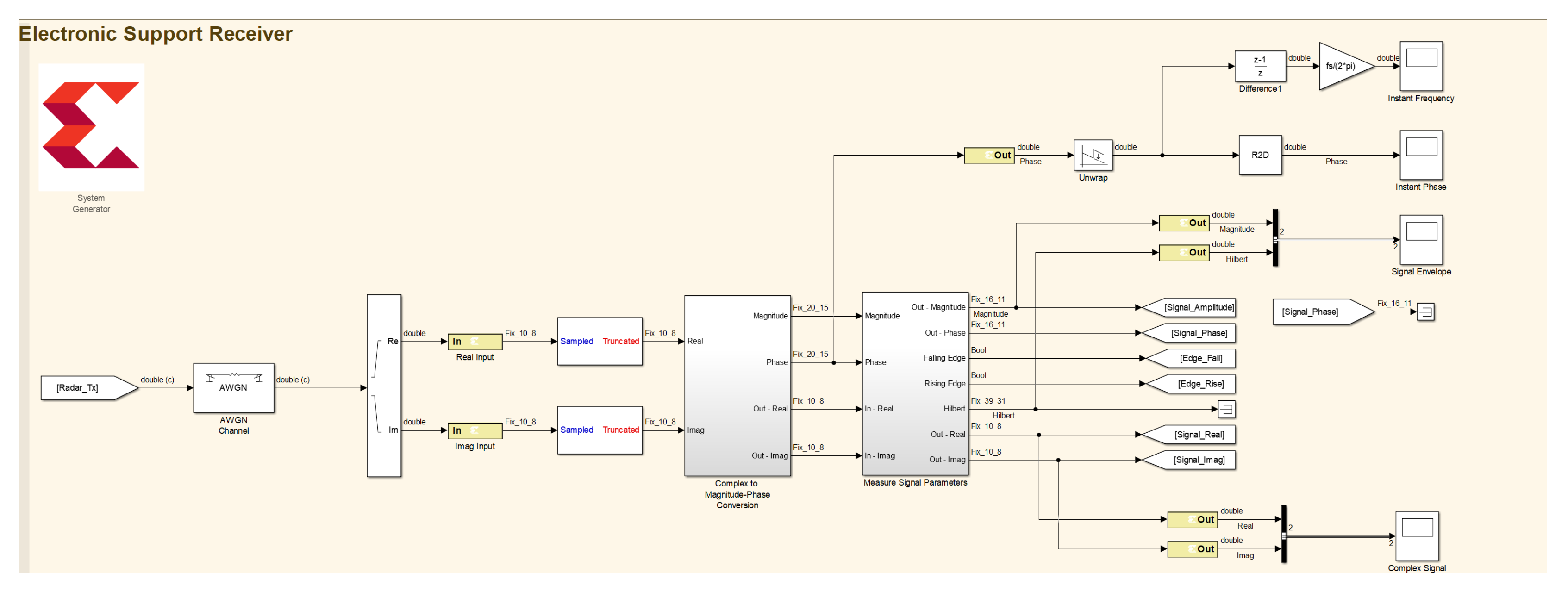
The jammer receiver, shown in Figure 4, performs the following functions: radar pulse detection of leading edge, radar pulse detection of falling edge, and formatting of the sampled signal in a two’s compliment fixed point word. The detection of the rising edge and falling edge are used as “triggers” to control the writing of the pulse to the DRFM system.

The first step involves converting the received double floating point I-Q signal to a digital fixed point version. This is performed first by adding White Gaussian Noise (WGN) at an adjustable Signal-to-Noise Ratio (SNR), then using the Xilinx Input blocks to convert the signal to a fixed point representation. The signal was sampled at the simulation period of 20 ns, using a 10 bit representation with the binary point at the 8th bit.

To allow for the system to be modeled using a variety of ADC resolutions, an adjustable truncation sub-system was added after the ADC conversion. While the choice of ADC resolution could have been made at the Xilinx input, and actually simplified the design in the process, the choice was made to model it afterward to allow for integration with the 10-bit ADC on the FPGA daughter card in the future.

Following the ADC sampling, the signal was converted to an amplitude and phase signal from an I-Q representation and fed into the detection block, shown in Figure 5. The detection block performed its function in the time domain, using a user adjustable threshold to find the leading and trailing edges of any incident pulses. To perform this function, the amplitude of the signal was differentiated, allowing for distinguishing the rising and falling edges. The output signals from this block were then fed into the PDW encoder sub-system, where detections of rising and falling edges were used to trigger the calculation of pulse parameters.

3.3. DRFM Model

The DRFM system has a simple task; it records a digitally sampled pulse to memory and “replays” the waveform at another time. At its heart, this function is performed by a two–port Random Access Memory (RAM) that can simultaneously write a signal to memory and read a signal from memory, as long as the read and write addresses are not identical.

The DRFM systems used in this paper are shown in Figure 6, and implemented simultaneously in amplitude and I-Q forms to facilitate testing, with an 18-bit address space of dual port memory on the FPGA. The resulting system could record up to 5.242 ms of pulse samples at the 20 ns sample period.

The DRFM sub-system is in many ways the simplest component of the jammer receiver, as its sole function is to record detected pulses to a RAM sub-system. The detection process, outlined in the previous sub-section, creates triggers for the rising and falling edges, which initiates and stops the process, respectively, of recording the pulse to memory. In the case of the I-Q model, shown in Figure 7, two identical DRFM sub-systems are used for each data stream, whereas for the amplitude DRFM, only a single DRFM sub-system is used.

The dual port RAM would normally be used to simultaneously record pulses and play them back to support the generation of ECM during a look-through operation. In this case, as the pulse repeater model was used, it wrote the received waveform to memory and simultaneously retransmitted the results.

3.4. Signal Correlator

To support testing the DRFM system, a correlator was used for each waveform: the transmitted radar signal, the amplitude DRFM, and the I-Q DRFM. Shown in Figure 8, outside of a time delay to align the transmitted signal with the DRFM signals (these were delayed while propagating through the DRFM), all three waveforms had the exact same operation performed on them.

The three waves were correlated with the signal that was transmitted using a Finite Impulse Response (FIR) filter implementation of the correlator, with an order of 500 in all of the cases examined in this paper. In the case of the radar signal, this provides the zero Doppler cut of the ambiguity function, which was used as a reference point for the distorted DRFM signals.

4. DRFM Performance Results

To understand how DRFM performance changed with the system architecture and the waveforms it encountered, a comparison of received and transmitted waveforms was conducted using a correlation. In radar terminology, the correlation was the matched filter response, specifically, the zero Doppler cut of the ambiguity function

$$\chi (\tau ,f)={\int }_{-\infty }^{\infty }s\left(t\right)s^{*}(t-\tau )e^{j2\pi ft}dt$$

(1)

where $s\left(t\right)$ is the waveform, f is the frequency, and $\tau$ is a dumby variable [21]. The implementation used to measure the DRFM system performance is equivalent to

$$\chi =\sum _{m=-\infty }^{\infty }x\left(n\right)h^{*}(n-m)$$

(2)

where $x\left(n\right)$ is the received waveform, and $h\left(n\right)$ is the transmitted waveform.

The output of the correlators was a 2-D plot showing the compressed waveform for the correlation of the transmitted waveform, along with various distortions for DRFM variants. However, the primary metrics of concern for the DRFM system performance were the signal processing loss compared to the ideal case (the autocorrelation), and the change in time delay of the peak of the compressed DRFM signal.

To understand the various factors that might affect processing gain and time delay, the performance of the DRFM system was evaluated under a variety of different conditions, including the ADC resolution, DRFM receiver SNR, waveform time-bandwidth product, and the I-Q vs. amplitude DRFM models.

4.1. Effects of DRFM Coherence and Radar Waveforms

The most major difference between DRFM implementations is the use of an envelope DRFM, recording the radar pulse amplitude but not its phase, and a full I-Q DRFM that replicates the in-phase and quadrature components of the received signal. This was particularly interesting as when a radar signal with a matched filter receives the envelope signal, how the two interact was not well established.

The effect of the amplitude and I-Q DRFM systems was compared by using two waveforms: a Linear Frequency Modulated (LFM) wave, and a 13-bit Barker code. In all cases, the SNR in the ES receiver was set to 40 dB, and the ADC resolution to 10 bits; this was done to distinguish the jammer and radar wave without emphasizing the effects of thermal and quantization noise.

The results for the LFM signal are shown in Figure 9, using a 10 μs pulse and with a 5 MHz bandwidth to replicate a common radar signal. The transmitted signal and jammer signal are clearly very similar at the output of the correlator, with only minor changes in the side-lobes and effectively no loss in processing gain or change in time delay.

However, the amplitude signal behaved significantly differently, as the correlation is comparing a square wave with a component of the LFM signal, resulting in the following variation of Equation (2)

$$\chi =\sum _{n=0}^{N-1}{e}^{j2\pi \frac{B}{{\tau }_p}{\left(n{t}_s\right)}^2}$$

(3)

where $N={\tau }_p/t_s$ is the number of samples in the pulse, B is swept frequency bandwidth, $t_s$ is the sample period, and ${\tau }_p$ is the pulse width. The output of the correlator makes sense in this context, as the initial oscillation is swept over the frequency range, the ripple in the envelope can be seen to change in Figure 9, resulting in a peak at the trailing edge.

The difference between the ideal and amplitude variant of the signal is a loss of $7.5$ dB in processing gain but with a peak located 8.5 μs later than the I-Q variant. While both these factors are important, the loss in signal processing gain was expected and can be compensated for by increasing the jammer power. The range delay is more problematic, as it results in a target appearing 1.3 km farther away, likely well outside the range gate of a tracking radar.

Interestingly, the power spread by the amplitude DRFM signal over a much larger range will flood any range of bins with likely sufficient power for a target detection in a search radar. In a tracking radar, it would also create significant energy, but inside the range gates and any possible guard gates as well. These two factors will affect countermeasure design, principally by shifting any pulses transmitted by the jammer in time to adjust for the artificial delay in a range caused by the matched filter and the unmodulated pulse.

For comparison, the same experiment was performed with a 13-bit Barker code, shown in Figure 10, as was done for the LFM waveform. The results were similar, but less pronounced, with only a 5-dB loss in processing gain, as a result of the significant difference in the time-bandwidth product (50 for the LFM wave, and 13 for the Barker code). The range delay displayed a less rippled effect, with peaks and troughs corresponding to the waveform’s side-lobes. The results of all the simulations from this sub-section are summarized in

Table 1. Complex and envelope DRFM comparison.

	${\mathit{G}}_{\mathit{p}}$	$\mathbf{\Delta }\mathit{t}$	SLL
LFM Complex	≈0 dB	≈0 $\mathsf{\mu }$s	5.0 dB
LFM Envelope	$-8.0$ dB	$8.5\mathsf{\mu }$s	1.0 dB
PSK Complex	≈0 dB	≈0 $\mathsf{\mu }$s	11 dB
PSK Envelope	$-4.0$	$6.2\mathsf{\mu }$s	1.0 dB

.

4.2. Effects of DRFM Receiver Signal-to-Noise Ratio

A significant concern in effectively recording a radar signal to the DRFM and replicating it is the presence of noise in the receiver corrupting the received waveform. To evaluate its effects, the scenario from the previous sub-section was modeled using only the I-Q DRFM under a variety of SNRs, from −10 to 20 dB, with the noise represented as Additive White Gaussian Noise (AWGN).

The effects can be seen for the LFM and PSK waveforms in Figure 11 and Figure 12, respectively. The PSK example, with its lower processing gain, offers a slightly better visualization of the impact of noise. At 20 dB of SNR, the PSK waveform is behaving as its autocorrelation would predict, with a main lobe and a gradually descending series of time-domain side-lobes. As the SNR is decreased, the side-lobe levels increase, effectively decreasing the dynamic range, and raising the noise floor. In both the LFM and PSK cases, there is little to no difference in signal processing gain across the various levels of AWGN. The results are summarized in

Table 2. Signal-to-noise ratio DRFM comparison.

	SNR (dB)	${\mathit{G}}_{\mathit{p}}$ (dB)	$\mathbf{\Delta }\mathit{t}$	SLL (dB)	Noise Floor (dB)
LFM	20	≈0	≈0	5	3
	10	≈0	≈0	5	7
	0	≈0	≈0	5	11
	−10	≈0	≈0	5	14
PSK	20	≈0	≈0	11	14
	10	≈0	≈0	11	12
	0	≈0	≈0	11	10
	−10	≈0	≈0	9	7

.

The surprisingly high amount of gain seen in all the examples in Figure 11 and Figure 12 can be linked to the lack of straddle loss. As the system is sampled at a much higher rate than necessary in the jammer system, where instantaneous bandwidths will often exceed 1 GHz, straddle loss is minimized. At the same time, straddle loss was not modeled in order to isolate other factors.

Recognizing the effects of moderate SNR values in the EW receiver seem unconcerning, the issue is more problematic when a DRFM jammer often has a bandwidth of 1 GHz. Relative to the moderate bandwidths seen in threat emitters, typically less than 20 MHz, the SNR can be relatively low in the DRFM, even when receiving sufficient power for detection.

4.3. Effects of DRFM ADC Resolution

One of the principle advances in EW receivers over the last 30 years has been the increasing speed and resolution of analogue-to-digital converters (ADC). The initial DRFM systems often relied upon mono-bit ADCs, capable of high speeds but only a single bit, which made them very sensitive to the threshold detection level. Modern ADCs are capable of much more, with most contemporary EW systems operating with ADCs sampling at giga-samples per second and in excess of 10-bits of resolution.

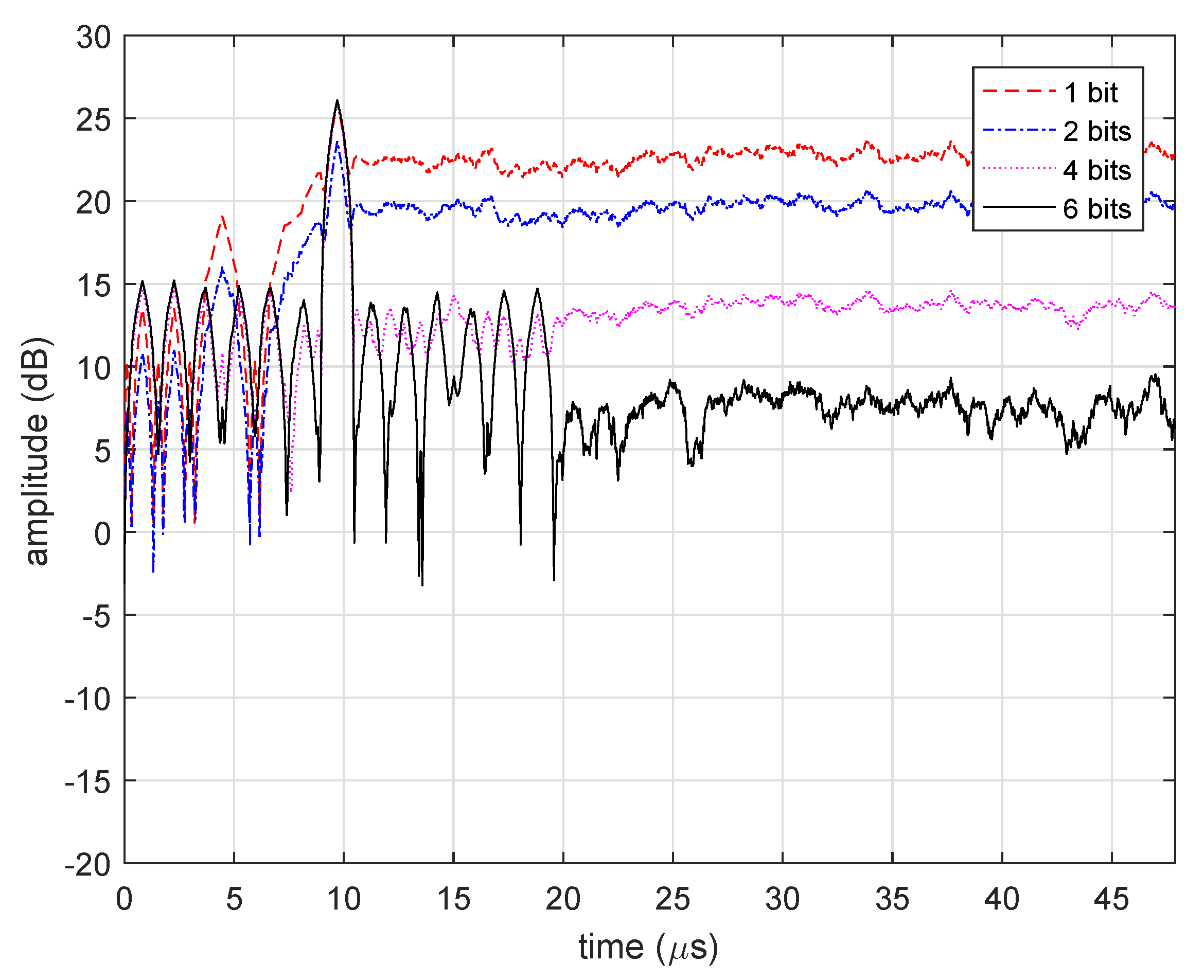
To understand the effects of the ADC resolution on DRFM performance, it was varied across a number of simulations, with the system implemented at 1, 2, 4, and 6 bits of resolution. In this case, only the I-Q DRFM was evaluated, with the system presenting surprisingly good results in replicating the radar waveform; see Figure 13 and Figure 14.

The results for the LFM and PSK waveforms are summarized in

Table 3. ADC resolution DRFM comparison.

ADC Bits	1	2	4	6
SLL—LFM	$-9$ dB	$-12$ dB	$-18$ dB	$-22$ dB
SLL—PSK	$-3$ dB	$-6$ dB	$-12$ dB	$-12$ dB

, comparing side-lobe levels for the various ADC resolutions. However, the major impact of the change in ADC resolution across the waveforms was the increased noise floor and corresponding reduction in dynamic range. The impact on dynamic range is not surprising as the number of bits in an ADC has a direct impact on the dynamic range in any receiver.

For the Barker code, the single bit system is well suited to recording the PSK waveform as it is essentially making a detection decision with each bit of either a “1” or a “0” present in both I/Q channels. Similarly, the LFM waveform is operating at sufficient speed that the change in phase is recorded. Both figures show this effect breaks down as the signal in the side lobes, as the low ADC resolution values have insufficient dynamic range to replicate these characteristics of the matched filter.

The lack of straddle loss in the model, discussed in Section 4.2, is another contributing factor in Figure 13 and Figure 14. Without the straddle loss at the DRFM receiver and matched filter, the two signals maintain the same set of original samples with distortion, not two asynchronous set of samples.

4.4. Effects of Waveform Time-Bandwidth Product

The last factor evaluated was the time-bandwidth product of the radar waveform received by the DRFM, defined here as:

$$\varrho =\tau \beta$$

(4)

where $\tau$ is the pulse width, and $\beta$ is the bandwidth; in order to understand the effects of $\varrho$ on the amplitude and I-Q DRFM systems. In both cases of the DRFM, an LFM signal was chosen due to the ease of scaling the time-bandwidth product compared to a Barker code.

The results for a 10 μs pulse with 1, 2, 5, and 10 MHz bandwidths are shown in Figure 15 and Figure 16. The I-Q DRFM clearly illustrates the $sin\left(x\right)/x$ pattern [21], with the expected reduction in main lobe width and decrease in side lobe levels as the bandwidth increases.

The more interesting effects occur in Figure 15 for the amplitude DRFM, where the replicated envelope pulse is slid over the LFM waveform during the correlation. The result is a ripple over the pulse that changes with the frequency of the LFM waveform. As the frequency increases, the pulse ripple decreases.

The results of these figures are summarized in

Table 4. LFM signal bandwidth comparison.

	Envelope		Complex
Bandwidth	$\mathbf{\Delta }\mathit{t}$($\mathsf{\mu }$s)	${\mathit{G}}_{\mathit{p}}$(dB)	$\mathbf{\Delta }\mathit{t}$($\mathsf{\mu }$s)	${\mathit{G}}_{\mathit{p}}$(dB)	SLL (dB)
1 MHz	7.5	$-4$	≈0	≈0	$-6$
2 MHz	8.5	$-5$	≈0	≈0	$-9$
5 MHz	9.5	$-8$	≈0	≈0	$-12$
10 MHz	10.0	$-9$	≈0	≈0	$-15$

. While not a linear response, the time delay and processing gain loss increase with an increase in signal bandwidth in an envelope DRFM. In a complex DRFM, recording the I/Q signal, the processing gain and time delay remain stable, but the side-lobe levels increase inversely with the signal bandwidth.

5. Multiple Scatterer DRFM

5.1. Multiple Scatterer Targets

As the inevitable cycle of innovation in Electronic Countermeasures (ECM) and Electronic Counter-Counter Measures (ECCM) continues, current forms of ECCM, such as non-cooperative target recognition, have limited the effectiveness of the DRFM architectures discussed so far [22]. The primary limitation in conventional DRFM jammers is the inability to accurately replicate the skin return of a target, as only a single signal is retransmitted at one time. In reality, the skin return of a target, such as an aircraft or ship, is the sum of a large number of signals, all with slightly different delays, phases, and Doppler shifts.

As an example, the RCS of a single cylinder is shown in Figure 17, a set of the same cylinder is then randomly distributed using a Gaussian distribution with a mean of zero and standard deviation of two, shown in Figure 18. Unfortunately, modern radars use capabilities such as NCTR, measuring not just the amplitude and Doppler shift of a single signal, but the combination of the amplitude and phase, including the individual Doppler shift of each scatterer.

For example, the jet engine of an aircraft can cause an effect on the scattered radar wave known as Jet Engine Modulation (JEM) where an amplitude modulation of the received signal power occurs with each rotational period of the turbine.

The effects of the multiple scatterers and their individual contributions to the received waveform can be expressed as a sum of the signals:

$$y\left(t\right)=\sum _{n=1}^N{\alpha }_{n}x\left(t-t_n\right)e^{-j{\omega }_{n}t}$$

(5)

where ${\alpha }_n$ is the amplitude, $t_n$ is the delay, and ${\omega }_n$ is the Doppler shift. Unfortunately, this system will vary with a variety of factors, such as the angle-of-arrival, frequency, and polarization, allowing the received signal to be expressed as a function of these factors:

$$y\left(t,\sigma \right)=\sum _{n=1}^N{\alpha }_n\left(\sigma \right)x\left(t-t_n\left(\sigma \right)\right)e^{-j{\omega }_n\left(\sigma \right)t}$$

(6)

where $\sigma$ is a set of the following variables:

$$\sigma =\langle \theta ,\varphi ,f,\widehat{\rho }\rangle$$

(7)

containing the azimuth, $\theta$, the elevation, $\varphi$, the frequency, f, and the polarization, $\rho$.

5.2. Multiple Scatterer DRFM Implementation

To resolve the issue of multiple scatterer replication in DRFM systems, a new architecture is needed that can replicate Equation (6). That is to say, create not just a single return signal but a superimposed set of jammer signals, which vary with angle-of-arrival, frequency, and polarization.

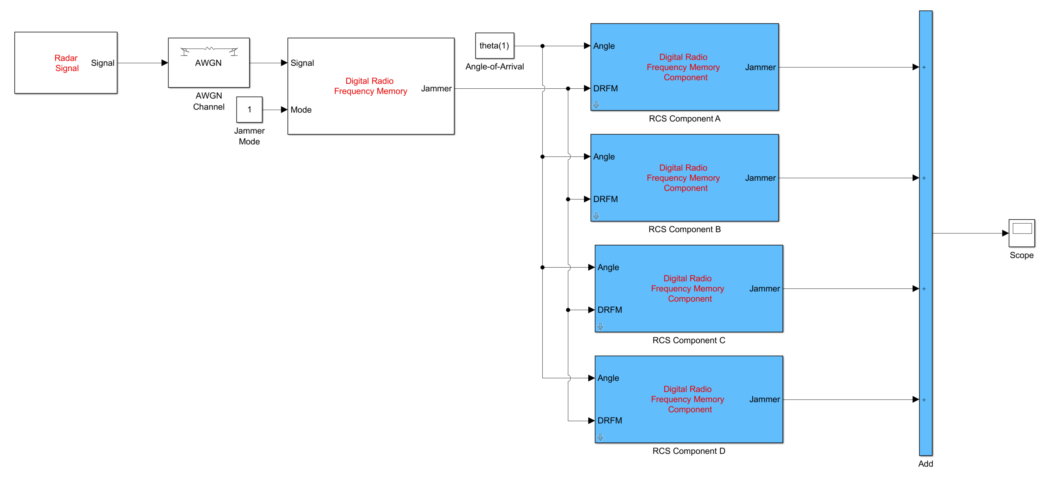
A version of this multiple scatterer DRFM was developed and implemented in System Generator and tested using a Kintex-7 FPGA, as shown in Figure 19. However, for simplicity of illustration, the complexity was limited to four scatterers with the signal only varying with the angle of arrival. Expanding on the architecture to replicate N-scatterers that vary with the azimuth, elevation, frequency, and polarization while not trivial, only requires scaling the number of RCS components for each scatterer and switching to a four dimensional look-up table to store the values for every possible combination of variables.

The DRFM shown in Figure 19 adapted the I/Q DRFM system shown in Section 3.3, with several modifications. The received signal is stored in the two-port RAM and replayed with the appropriate modification to generate the desired EA (such as range-gate pull-off, inverse-gain jamming, cover pulses, etc.). However, after the DRFM generates the waveform to be transmitted, it splits into a series of subsystems to replicate the delay, amplitude, and frequency shift of each individual scatterer. The modifications for each scatterer are determined from a look-up table based on previous measurements. Finally, the waveform generated from each synthetic scatterer in the DRFM system is superimposed and sent to the transmitter.

5.3. Multiple Scatterer DRFM Results

In the example discussed here, the system modeled using the multi-scatterer DRFM contained a set of four sources, each with a progressive amplitude, time delay, and Doppler shift. The multi-scatterer waveform results are plotted in Figure 20, where in amplitude alone, the two waveforms are easily distinguished. The individual contributions of the scatterers can be seen in Figure 21.

The complexity of implementing a DRFM jammer using this architecture is not actually in the electronics but in gathering the extensive data to build the database for the look-up table. Specifically, it would require a range or anechoic chamber where the jammer platform could be measured across all variables: azimuth, elevation, frequency, etc.

6. Conclusions

This paper explored a variety of effects on DRFM system performance against a modern coherent radar, including architecture, ADC resolution, received SNR, and the signal time-bandwidth product. These factors are of particular importance to the science of designing an effective Electronic Attack (EA), and how an EA must be adjusted to compensate for these distortions.

The key factor in effective EAs is the Jammer-to-Signal Ratio (JSR) as—while it often does not need to exceed 3 to 6 dB—falling short of the required number can be fatal. While each scenario is unique, the factors discussed in detail here all weigh on the processing loss of the DRFM system and will affect the required jammer transmit power to achieve the requisite JSR.

Similarly, the jammer power must be placed in the appropriate tracking gate or it is wasted, having no effect on the JSR. The guidance developed here on how the effective range delay changes with an envelope DRFM with the signal bandwidth and other factors, is a critical adjustment when conducting Range Gate Pull-Off (RGPO) attacks or similar techniques.

Finally, the paper proposed and implemented a novel DRFM architecture capable of generating effective EA against radars with sophisticated forms of EP.