Article

Novel Active Disturbance Rejection Control Based on Nested Linear Extended State Observers

by
Wameedh Riyadh Abdul-Adheem
1,
Ahmad Taher Azar
2,3,*,
Ibraheem Kasim Ibraheem
1 and
Amjad J. Humaidi
4
1
Department of Electrical Engineering, College of Engineering, University of Baghdad, Al-Jadriyah, Baghdad 10001, Iraq
2
Robotics and Internet-of-Things Lab (RIOTU), Prince Sultan University, Riyadh 11586, Saudi Arabia
3
Faculty of Computers and Artificial Intelligence, Benha University, Benha 13518, Egypt
4
Department of Control and Systems Engineering, University of Technology, Baghdad 10001, Iraq
*
Author to whom correspondence should be addressed.
Appl. Sci. 2020, 10(12), 4069; https://doi.org/10.3390/app10124069
Submission received: 13 April 2020 / Revised: 5 June 2020 / Accepted: 8 June 2020 / Published: 12 June 2020
(This article belongs to the Special Issue Nonlinear Control: Theory and Applications)

Abstract

:

Featured Application

The proposed Novel Active Disturbance Rejection Control can be applied to various real-world models such as Permanent Magnet DC (PMDC) motors, Permanent Magnet Synchronous Motors, Differential Drive Mobile Robots (DDMR), winged-cone Generic Hypersonic Vehicles (GHV), and spacecraft systems. Authors are encouraged to provide a concise description of the specific application or a potential application of the work. This section is not mandatory.

Abstract

In this paper, a Novel Active Disturbance Rejection Control (N-ADRC) strategy is proposed that replaces the Linear Extended State Observer (LESO) used in Conventional ADRC (C-ADRC) with a nested LESO. In the nested LESO, the inner-loop LESO actively estimates and eliminates the generalized disturbance. Increasing the bandwidth improves the estimation accuracy which may tolerate noise and conflict with H/W limitations and the sampling frequency of the system. Therefore, an alternative scenario is offered without increasing the bandwidth of the inner-loop LESO provided that the rate of change of the generalized disturbance estimation error is upper bounded. This was achieved by the placing of an outer-loop LESO in parallel with the inner one that estimates and eliminates the remaining generalized disturbance originating from the inner-loop LESO due to bandwidth limitations. The stability of LESO and nested LESO was investigated using Lyapunov stability analysis. Simulations on uncertain nonlinear single-input-single-output (SISO) system with time-varying exogenous disturbance revealed that the proposed nested LESO could successfully deal with a generalized disturbance in both noisy and noise-free environments, where the Integral Time Absolute Error (ITAE) of the tracking error for the nested LESO was reduced by 69.87% from that of the LESO.

Graphical Abstract

1. Introduction

The performance of a control system is excessively affected by system uncertainties, such as exogenous disturbances, unmodelled dynamics, and parameter perturbations. Simultaneously guaranteeing disturbance rejection and good tracking performance in light of the existence of large uncertainties complicates the design of any controller that aims to address these objectives. Accordingly, anti-disturbance methods with both external-loop controllers and internal-loop estimators have been comprehensively utilized. The precision of such controls mainly depends on the accuracy of the observer in the internal-loop, this type of controller is called “model-free controller” in contrast to other controllers that require the dynamics of the system, e.g., disturbance-observers-based control [1]. There have been various observer design philosophies posited, including fuzzy observers, sliding mode observers, unknown input observers, perturbation observers, equivalent input observers, extended state observers, and disturbance observers. Of these observers, the Extended State Observer (ESO) was originally suggested by Han [2]; it is often favoured because, in terms of design, it requires the minimum information from the system. It estimates the internal states of the system, system uncertainties, and exogenous disturbances, and it can also be used to design a state feedback controller. Based on this, an ESO is considered an essential part of the active disturbance rejection control paradigm. ESO-based control design has thus been widely examined in recent years [3,4]. The basic principle behind the operation of ESO is to augment the mathematical model of the nonlinear dynamical system with an additional virtual state that describes all the unwanted dynamics, uncertainties, and exogenous disturbances, which is termed “generalized disturbance”. This virtual state, together with the states of the dynamic system, is observed in real-time using the ESO. This form of control design has been applied to a broad range of systems due to its model-independent operation. Initially, each ESO was constructed with nonlinear gains; however, it is more realistic to design and tune the ESO using tuneable linear gains, as proposed in [5]. Two signals, the input and the output of the nonlinear system, thus feed the ESO with information [6]. An ESO-based control system design offers generally good performance due to the simplicity of design of ESO, which offers a need for minimum information, high precision of convergence, and fast-tracking capabilities [7]. In [8], ESO is tested on the nonlinear kinematic model of the Differential Drive Mobile Robot (DDMR). In [9], a general ESO-based control technique for nonchain integrator systems with mismatched disturbances was proposed. Recently, numerous control problems in various fields have also been effectively resolved by utilizing the ESO technique, including permanent magnet synchronous motor(PMSM) control [10], and attitude control of an aircraft [11]. The authors in [12] introduced an ESO-based dynamic sliding-mode control for high-order mismatched uncertainties with applications in motion control systems, and this also presented excellent tracking performance. In [13], an improved nonlinear ESO was proposed which achieved an outstanding performance in terms of smoothness in the control signal which leads to less control energy required to attain the desired performance. Techniques other than classical ones for dealing with measurement noise are proposed in the literature, e.g., authors of [14,15] have proposed a novel class of Adaptive ESOs (AESOs) with time-varying observer gains. As a result, the proposed AESO combines both the advantages of nonlinear extended state observer (NESO) and Linear Extended State Observer (LESO) and provided more extra design flexibility than LESO. Techniques different from ESO based estimation methods like time-delay estimators to estimate the generalized disturbance are proposed in [16,17]. Moreover, disturbance rejection approaches considering robust controllers combined with disturbance observer can be found in [18,19].
The weak points of the aforementioned methods lie in the following:
(1)
For the LESO to increase the estimation accuracy, the bandwidth of the LESO has to be increased, which tolerates noise and leads to hardware difficulties. Additionally, the LESO suffers from a peaking phenomenon due to large gain values.
(2)
For the nonlinear ESO, the performance will abruptly deteriorate when the amplitude or derivative of the generalized disturbance goes large to a certain degree [20]. Moreover, stability analysis and performance analysis are very complicated for the nonlinear ESO.
(3)
For other classes of observers like the AESO, the parameter tuning process becomes more time-consuming as the observer order goes higher.
In this paper, we offer a novel simple structure based on LESO, namely, the nested LESO, which combines the advantages of both linear and nonlinear ESOs. It consists of two LESOs connected in parallel sharing the same plant output. The proposed observer efficiently estimates the generalized disturbance without increasing the observer bandwidth and requires fewer computations for parameter tuning since it is built from LESOs which needs a single parameter to be tuned, i.e., the LESO bandwidth. Moreover, due to its linear structure, the proposed nested LESO inherits the simplicity of the LESO stability analysis, while the performance evaluation of the closed-loop system of an uncertain nonlinear signle-input-single-output (SISO) system is achieved very easily with the proposed nested LESO.
An outline of this paper’s contents and organisation follows. Section 2 presents the problem statement and contribution of this work. Section 3 briefly presents the concepts behind Active Disturbance Rejection Control (ADRC). A description of the proposed nested LESO and the relevant stability tests are included in Section 4. The numerical simulations verifying the validity of the proposed configuration are provided in Section 5. Finally, the conclusion is given in Section 6, along with recommendations for future work.

2. Problem Description and Contribution

2.1. Problem Description

Consider an n-th dimensional uncertain nonlinear SISO system,
{ x ˙ 1 ( t ) = x 2 ( t ) ,   x 1 ( 0 ) = x 10 x ˙ 2 ( t ) = x 3 ( t ) ,   x 2 ( 0 ) = x 20 x ˙ n ( t ) = f ( t , x 1 ( t ) , x 2 ( t ) , , x n ( t ) ) + w ( t ) + u ( t ) , x n ( 0 ) = x n 0 y ( t ) = x 1 ( t )
where u ( t ) C ( R , R ) is the control input, y ( t ) is the measured output, f C ( R n , R ) is an unknown function, w ( t ) C ( R , R ) is the exogenous disturbance, x ( t ) = ( x 1 ( t ) , x 2 ( t ) , , x n ( t ) ) is the state vector of the system, and x ( 0 ) = ( x 10 , x 20 , , x n 0 ) is the initial state. L ( t ) = f + w ( t ) is therefore the “generalized disturbance” [1]. By adding the extended state x n + 1 ( t ) = def = L ( t ) = f + w ( t ) to Equation (1), it can be written as,
{ x ˙ 1 ( t ) = x 2 ( t ) ,   x 1 ( 0 ) = x 10 x ˙ 2 ( t ) = x 3 ( t ) ,   x 2 ( 0 ) = x 20 x ˙ n ( t ) = x ( n + 1 ) ( t ) + u ( t ) , x ( t ) ) = x n 0 x ˙ n + 1 ( t ) = f ˙ ( t , x 1 ( t ) , x 2 ( t ) , , x n ( t ) ) + w ˙ ( t ) , x n + 1 ( 0 ) = x n + 1 , 0 y ( t ) = x 1 ( t )
Let Δ ( t ) = L ˙ ( t ) = d L d t ; it is required to estimate the state vector x ( t ) and the generalized disturbance x n + 1 ( t ) of the nonlinear system (Equation (2)) in the presence of the system uncertainties, exogenous disturbances, and measurement noise. To solve the above estimation problem, a conventional LESO is given as per [1]:
{ x ^ ˙ 1 ( t ) = x ^ 2 ( t ) + β 1 ( y ( t ) x ^ 1 ( t ) ) x ^ ˙ 2 ( t ) = x ^ 3 ( t ) + β 2 ( y ( t ) x ^ 1 ( t ) ) x ^ ˙ n ( t ) = x ^ n + 1 ( t ) + u ( t ) + β n ( y ( t ) x ^ 1 ( t ) ) x ^ ˙ n + 1 ( t ) = β n + 1 ( y ( t ) x ^ 1 ( t ) )
where β i is a constant observer gain to be tuned, i = 1, 2, … n + 1. The LESO gains β i are selected as:
β i = a i ω 0 i ,   i = 1 , 2 , , n + 1
where ω o is the LESO bandwidth, β i , i = 1 , 2 , , n + 1 are selected such that the characteristic polynomial, s n + 1 + β 1 s n + + β n s + β n + 1 = ( s + ω 0 ) n + 1 is Hurwitz. The binomial coefficients a i , i = 1 , 2 , , ρ + 1 are defined as [21]:
a i = ( n + 1 ) ! i ! ( n + 1 i ) ! ,      1 i n + 1
However, for perfect estimation of the system states x ( t )   and the generalized disturbance x n + 1 ( t ) , large LESO bandwidth ω o   is required. Thus, tolerating noise and increasing H/W complexities. In contrast, reducing ω o leads to large estimation errors x i ( t ) x ^ i ( t ) , 1 i n + 1 . Consequently, to solve the above estimation problem with minimum estimation errors as compared to that of LESO, a nested LESO is proposed to estimates x ( t )   and x n + 1 ( t ) without increasing ω o .

2.2. Paper Contribution

In this paper, a novel ADRC is constructed by connecting a second LESO in parallel with an original LESO (the inner LESO) to construct a nested LESO. The advantage of this configuration is that the second LESO estimates and eliminates the remaining generalized disturbance that eluded from the inner LESO due to bandwidth limitations. Its excellent performance becomes very evident when considered in terms of measurement noise. The proposed observer with nested structure differs from the state observer with a cascade structure, where the latter is just a state observer and used in special applications with delayed measurements such as the presence of an arbitrarily long delay in the output [22] or for position and attitude estimation of Unmanned Air Vehicles (UAVs) [23]. It should be emphasized that our main contribution is proposing a new structure to build a modified linear extended state observer by nesting two LESOs, sharing the same output rather than modifying the internal structure of the LESO. To the best of the authors’ knowledge, using double LESOs within the same ADRC structure, with applications in highly uncertain nonlinear systems, has not previously appeared in the literature.

3. Conventional Active Disturbance Rejection Control Problem

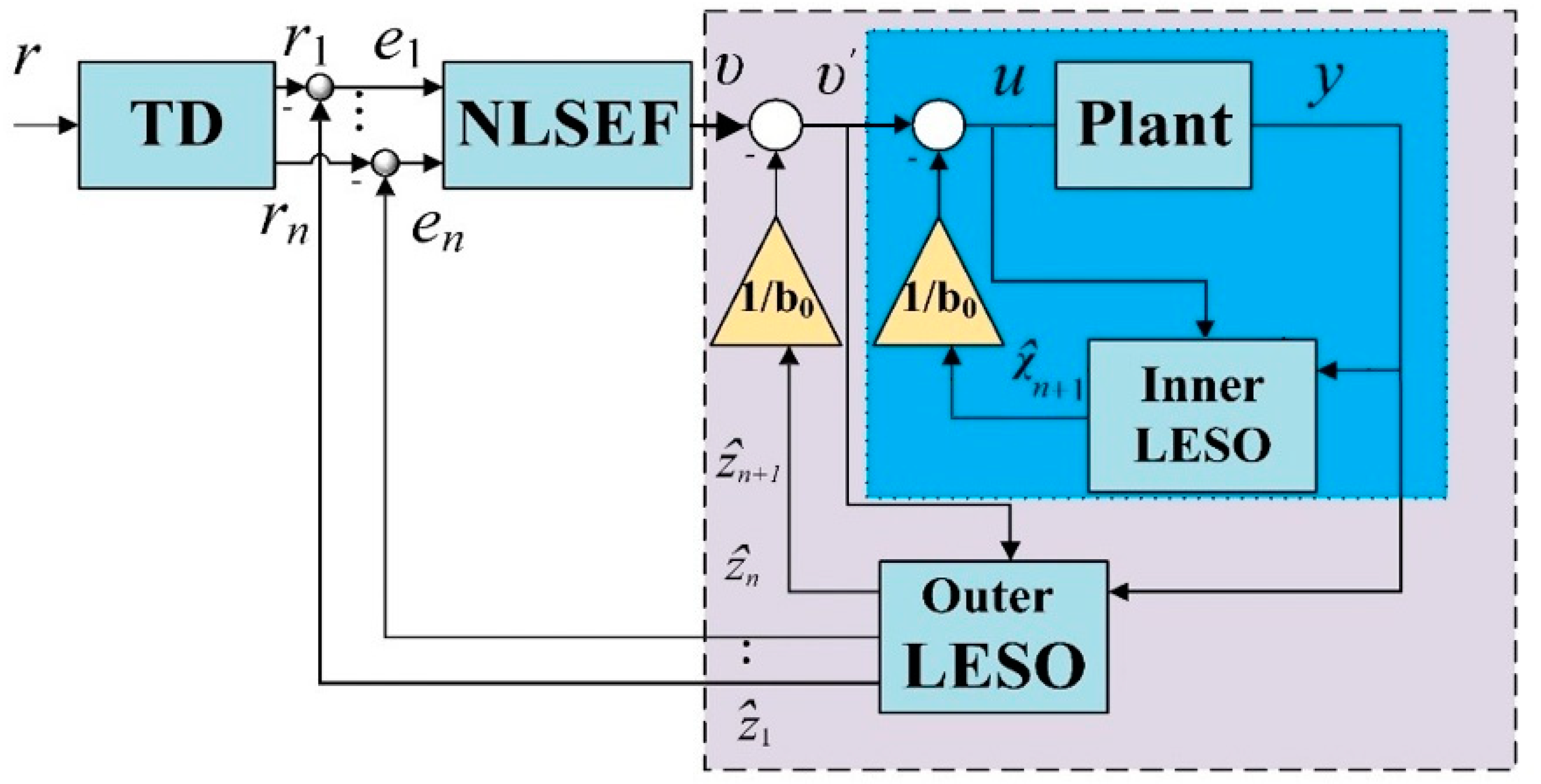
In ADRC, the model of the nonlinear system is extended with an additional virtual state variable, which lumps all of the unwanted dynamics, uncertainties, and disturbances that remain unobserved in the standard system into a single term known as “generalized disturbance”. In addition to estimating the states of the nonlinear system, the ESO performs online estimation and cancellation of this virtual state. In this scenario, the nonlinear system is converted into a chain of integrators, which allows the control system design to be simpler. Figure 1 demonstrations the structure of a Conventional ADRC, (C-ADRC) which contains three key parts: the Tracking Differentiator (TD), an Extended State Observer (ESO), and Nonlinear State Error Feedback (NLSEF) [24]. The tracking differentiator generates the required signal profile, which is the signal itself, free from noise, and a set of signal derivatives (first derivative, second derivative …). The NLSEF acts as a nonlinear combination of the error profile. The ESO function is as discussed in the introduction section [25].

3.1. Tracking Differentiator (TD)

In the tracking differentiator, the output profile of the nonlinear system, in Brunovsky canonical form [26], must track the transient profile of the reference signal to resolve the problem of set-point jump in the traditional proportional-integral-derivative (PID) controller as stated in the seminal work [2]. In this manner, when a rapid change occurs in the set point for any reason, the output signal of the plant will follow the output of the TD and will change gradually to reach the desired set-point, and the TD can be represented as [2]:
{ r ˙ 1 = r 2 r ˙ 2 = R   s i g n ( r 1 r ( t ) + r 2   | r 2 | 2 r )
where r1 is the tracking signal of the input r, and r2 is the tracking signal of the derivative of the input r. To speed up or slow down the system during transient effects, the coefficient R is adapted, making it application dependent [27]. Other versions of enhanced TD are proposed in [28,29,30,31].

3.2. Nonlinear State Error Feedback (NLSEF)

The linear weighting sum of the PID control is another limitation, involving as it does only the present, predictive, and accumulative errors, and omitting other important parameters that could enhance its performance [27]. In the seminal work [2], the following nonlinear control law was suggested [2]:
f a l ( e . α . δ ) = { e δ 1 α | x | δ | e | α s i g n ( e ) | x | δ
where α is a tuning parameter. The error signal, e, can thus reach zero more rapidly where α ˂ 1 [27]. Other forms of nonlinear control laws are suggested in [32,33,34,35].

3.3. Extended State Observer

Observers acquire data about the system states from its inputs and outputs progressively. Luenberger first recommended the rule of observers in [36], where it was concluded that the state vector of the system can be estimated by observing the input and output of the system. Subsequently, there have been numerous varieties of state observers outlined in the literature that rely upon the mathematical model of the system, including high gain observers and sliding mode observers [27]. The ESO was the first observer presented that was autonomous of the mathematical model and presented within the framework of ADRC. Furthermore, ESO has denoted estimators, which are considered a vital part of modern controls. The basic principle of the ESO is to observe the constituent parts of the generalized disturbance in real time, including model discrepancy, exogenous disturbances, and the unmodelled dynamics of the nonlinear system. Additionally, it compensates for unpredicted disturbances in the control signal. ESO can be classified into two types. The first is linear ESO, which is an extension of the Luenberger observer [36,37], where the equations of the ESO contain only the linear correcting terms in order to simplify the calculations. These terms manipulate the error between the actual states of the system and the estimated states in such a way that the error approaches zero. The second type is nonlinear ESO, where the error-correcting terms include a nonlinear function of the error. These nonlinear functions have the advantage of enhancing the estimation error more rapidly and smoothly than the linear ESO.
Two approaches are common for ESO tuning: the pole-placement approach, and the bandwidth-based method. If the end goal is to reduce the number of parameters of the ESO, the parameters of the ESO can be expressed as a function of the bandwidth of the ESO, allowing only a single parameter of the ESO to be chosen or tuned. Selecting a bandwidth that is too large leads to a drop in the estimation error that nevertheless remains within an acceptable bound [38]. Observer bandwidth is chosen to be sufficiently larger than the disturbance frequency and smaller than the frequency of the unmodelled dynamics [39]. However, the performance of the ESO will deteriorate if the bandwidth of the ESO is selected to be too low or too high. High values in the bandwidth of the ESO and the controller result in good tracking performance and rejection of exogenous disturbances. The side effects of adopting large values for bandwidth can thus be summarized as (1) measurement noise causing a degradation in output tracking, introducing chatter on the control signal [40]; (2) a worsening of the transient response of the ESO, as large values of bandwidth lead to what are known as high gain observers [41]; and (3) the possibility of some unmodelled high-frequency dynamics being activated beyond a certain frequency, causing inconsistency in the closed-loop system. The noise and sampling rates are considered the two main factors constraining increases in the bandwidth. Based on this, an appropriate estimator bandwidth ought to be chosen in coordination with the noise tolerance and tracking performance. The authors in [14] designed a new class of Adaptive ESO (AESO) in which the observer bandwidth varied with time to provide better performance than the LESO. The disadvantage of this method is that the parameter tuning may become more complex as AESO order increases [14]. To alleviate the peaking phenomenon caused by different initial values of the ESO, the small variable ε was designed as in [42]:
1 ε = { 100 t 3 0 t 1 100 t > 1
The ESO parameters are tuned using Evolutionary Algorithm (EA), optimization techniques like bacterial foraging optimization (BFO) and particle swarm optimization (PSO) rather than a manual process. Eventually, the ESO begins estimating these states. Consequently, the effect of lumped disturbances is cancelled and the controller actively compensates for the disturbances in real time [37].

4. Main Results

The innovative ADRC is constructed by adding an extra LESO, which shares an output signal with the plant to be controlled with an inner-loop LESO. The structure of the novel ADRC is presented in Figure 2. The inner LESO accomplishes the estimation of plant states and generalized disturbance. In a situation where a suitably low bandwidth ω 0 is selected for the inner LESO to reduce noise, the estimation of the generalized disturbance through the augmented state is associated with a relatively large estimation error, this situation is deeply considered in [43]. The outer-loop LESO will thus complete the rejection process by choosing an appropriate control law v that depends on the estimated generalized disturbance z ^ n + 1 .
Assumption A1.
The function L is continuously differentiable and there is a positive constant M such that Δ ( t ) is bounded by it, i.e.,
0 t sup   | Δ ( t ) | M
This assumption represents wide range of fast and slow disturbances which exist in many real-world applications.
Assumption A2.
There exist constants λ 1   a n d   λ 2 and positive definite, continuous differentiable functions V , W : n + 1 + such that
λ 1 | | y | | 2 V ( y ) λ 2 | | y | | 2
Letting W ( y ) = | | y | | 2 , we can assume
i = 1 ρ V i y i ( y i a i y 1 ) V y ρ + 1 a ρ + 1 y 1 W ( y )
The stability of the proposed nested LESO is conducted in the following steps. Firstly, demonstrating the stability of the inner-loop LESO by deriving the error dynamics of the system in Equation (1) and proving its stability using the Lyapunov function (Theorem 1). Secondly, deriving the state-space equation of the nonlinear system combined with the inner-loop LESO (dotted square in Figure 2 given by Equation (26). Then, proving that the derivative of the generalized disturbance estimation error e ˙ n + 1 is upper bounded by M , which is less than M defined in Assumption A1 (Lemma 1). Meanwhile, the stability analysis of the outer-loop LESO is demonstrated in Corollary 1 based on the results of Theorem 1. Finally, the stability analysis of the closed-loop system is given in Theorem 2.
Theorem 1.
Given the nonlinear plant (2) and the LESO in (3), then, the steady state estimation is given as
lim t | x i ( t ) x ^ i ( t ) | = 1 ω 0 n + 2 i 2 M λ 2 m a x ( P ) λ m i n ( P )
where x i ( t ) and x ^ i ( t ) , i { 1.2 . . n + 1 } denote the solutions of Equations (2) and (3) respectively, a i , i { 1 , 2 , n + 1 } are relevant constants, and ω 0 is the LESO bandwidth. Moreover, if ω 0   , then lim t | x i ( t ) x ^ i ( t ) | = 0 .
Proof. 
The proof is as follows, set
e i ( t ) = x i ( t ) x ^ i ( t ) ,   i { 1 , 2 , , n + 1 }
Subtracting Equation (3) from Equation (2), this gives
{ x ˙ 1 ( t ) x ^ ˙ 1 ( t ) = x 2 ( t ) ( x ^ 2 ( t ) + β 1 ( y ( t ) x ^ 1 ( t ) ) ) x ˙ 2 ( t ) x ^ ˙ 2 ( t ) = x 3 ( t ) ( x ^ 3 ( t ) + β 2 ( y ( t ) x ^ 1 ( t ) ) ) x ˙ n ( t ) x ^ ˙ n ( t ) = x n + 1 ( t ) + u ( t ) ( x ^ n + 1 ( t ) + u ( t ) +   β n ( y ( t ) x ^ 1 ( t ) )   ) x ˙ n + 1 ( t ) x ^ ˙ n + 1 ( t ) = Δ ( t ) β n + 1 ( y ( t ) x ^ 1 ( t ) )
where β i = a i ω 0 i , i { 1.2 . . n + 1 } are relevant constants. Direct computation shows that the estimation error dynamics satisfy
{ e ˙ 1 ( t ) = e 2 ( t ) β 1 e ( t ) e ˙ 2 ( t ) = e 3 ( t ) β 2 e ( t ) e ˙ n ( t ) = e n + 1 ( t ) β n e ( t ) e ˙ n + 1 ( t ) = Δ ( t ) β n + 1 e ( t )
and thus, the final form is:
{ e ˙ 1 ( t ) = e 2 ( t ) ω 0 a 1 . e 1 ( t ) e ˙ 2 ( t ) = e 3 ( t ) ω 0 2 a 1 . e 1 ( t ) e ˙ n ( t ) = e i n + 1 ( t ) ω 0 n a n . e 1 ( t ) e ˙ n + 1 ( t ) = Δ ( t ) ω 0 n + 1 a n + 1 . e 1 ( t )
Set
η i ( t ) = ω 0 n + 1 i e i ( t ω i 0 ) ,   i { 1 , 2 , , n + 1 }
or e i ( t ω 0 ) = 1 ω 0 n + 1 i η i ( t ) , then
{ d e 1 ( t ω 0 ) d t ω 0 = e 2 ( t ω 0 ) ω 0 a 1 . e 1 ( t ω 0 ) d e 2 ( t ω 0 ) d t ω 0 = e 3 ( t ω 0 ) ω 0 2 a 2 . e 1 ( t ω 0 ) d e n ( t ω 0 ) d t ω 0 = e n + 1 ( t ω 0 ) ω 0 n a n . e 1 ( t ω 0 ) d e n + 1 ( t ω 0 ) d t ω 0 = Δ ω 0 n + 1 a n + 1 . e 1 ( t ω 0 )
From Equation (15), d η i ( t ) d t = ω 0 n + 1 i d e i ( t ω 0 ) d t ω 0 d ( t ω 0 ) d t = ω i 0 n i d e i ( t ω 0 ) d t ω 0 can be derived. Then,
d e i ( t ω 0 ) d t ω 0 = 1 ω 0 n i d η i ( t ) d t
Both Equations (15) and (17) are substituted into Equation (16) and the result is
{ 1 ω 0 n 1 d η 1 ( t ) d t = 1 ω 0 n 1 η 2 ( t ) ω 0 a 1 . 1 ω 0 n η 1 ( t ) 1 ω 0 n 2 d η 2 ( t ) d t = 1 ω 0 n 2 η 3 ( t ) ω 0 2 a 2 . 1 ω 0 n η 1 ( t ) d η n ( t ) d t = η i n + 1 ( t ) ω 0 n a n . 1 ω 0 n η i ( t ) 1 ω 0 1 d η i , n + 2 ( t ) d t = Δ ω 0 n + 1 a n + 1 . 1 ω 0 n η 1 ( t )
The time-scaled estimation error dynamics are
{ d η 1 ( t ) d t = η 2 ( t ) a 1 η 1 ( t ) d η 2 ( t ) d t = η 3 ( t ) a 2 η 1 ( t ) d η n ( t ) d t n η n + 1 ( t ) a n η i ( t ) d η n + 1 ( t ) d t = Δ ω 0 a n + 1 . η 1 ( t )
Consider the candidate Lyapunov functions V , W : n + 1 + defined by V ( η ) = P η , η = η T P η , where η n + 1 and P is a symmetric and positive definite matrix. Suppose Assumption A2 (9) with λ 1 = λ m i n ( P ) and λ 2 = λ m a x ( P ) , where λ m i n ( P ) and λ m a x ( P ) are the minimal and maximal eigenvalues of P , respectively. Finding the derivative of V ( η ) w.r.t t along the solution of η in Equation (19), V ˙ ( η ) | a l o n g   ( 19 ) = i = 1 n + 1 V ( η ) η i η ˙ i ( t ) = i = 1 n + 1 V ( η ) η i ( η i + 1 ( t ) a i . η 1 ( t ) ) + V ( η ) η n + 1 ( Δ ω 0 a n + 1 . η 1 ( t ) ) . Then, V ˙ ( η ) | a l o n g   ( 19 ) = i = 1 n + 1 V ( η ) η i ( η i + 1 ( t ) a i . η 1 ( t ) ) + V ( η ) η n + 1 Δ ω 0 V ( η ) η n + 1 a n + 1 . η 1 ( t ) .
Based on Assumption A2, V ˙ ( η ) | a l o n g   ( 19 ) W ( η ) + V ( η ) η n + 1 Δ ω 0 . As V ( η ) λ m a x ( P ) | | η | | 2 and | V η n + 1 | | | V ( η ) η | | , then | V η ρ + 1 | 2 λ m a x ( P ) | | η | | . As V ( η ) λ m a x ( P ) | | η | | 2 = λ m a x ( P ) W ( η ) . Thus, W ( η ) V ( η ) λ m a x (   P ) . Finally, because λ m i n ( P ) | | η | | 2 V ( η ) , this leads to | | η | | V ( η ) λ m i n ( P ) . From Assumption A1, V ˙ i ( η i ) V ( η ) λ m a x ( P ) + M ω 0 2 λ m a x ( P ) V i ( η ) λ m i n ( P ) . As d d t V ( η ) = 1 2 1 V ( η ) V ˙ ( η ) , d d t V ( η ) 1 2 1 V ( η ) ( V ( η ) λ m a x ( P ) + M ω 0 2 λ m a x ( P ) V ( η ) λ m i n ( η ) ) . Thus,
d d t V ( η ) V ( η ) 2 λ m a x ( P ) + M ω 0 λ m a x ( P ) λ m i n ( P )
Solving ordinary differential Equation (20) gives,
V ( η ) 2 M λ 2 m a x ( P ) ω 0 λ m i n ( P ) ( 1 e t 2 λ m a x ( P ) ) + V ( η ( 0 ) ) e t 2 λ m a x ( P )
From Assumption A2, λ m i n ( P ) | | η | | 2 V ( η ) . This leads to | | η | | V ( η ) λ m i n ( P ) , then Equation (21) can be described as:
| | η ( t ) | | 1 λ m i n ( P )   ( 2 M λ 2 m a x ( P ) ω 0 λ m i n ( P ) ( 1 e t 2 λ m a x ( P ) ) + V ( η ( 0 ) ) e t 2 λ m a x ( P ) ) | | η | | ( t )   2 M λ 2 m a x ( P ) ω 0 λ m i n ( P ) ( 1 e t 2 λ m a x ( P ) ) + V ( η ( 0 ) ) λ m i n ( P ) e t 2 λ m a x ( P )
It follows from Equation (15) that | x i ( t ) x ^ i ( t ) | = 1 ω 0 n + 1 i | η i ( ω 0 t ) | | x i ( t ) x ^ i ( t ) | 1 ω 0 n + 1 i | | η ( t ) | | . Thus, by using Equation (20),
| x i ( t ) x ^ i ( t ) | 1 ω 0 n + 1 i ( 2 M λ 2 m a x ( P ) ω 0 λ m i n ( P ) ( 1 e t 2 λ m a x ( P ) ) + V ( η ( 0 ) ) λ m i n ( P ) e t 2 λ m a x ( P ) )
Finally,
lim t | x i ( t ) x ^ i ( t ) | 1 ω 0 n + 2 i 2 M λ 2 m a x ( P ) λ m i n ( P )
It is clear that when ω 0   , lim t | x i ( t ) x ^ i ( t ) | = 0  □
Based on the result of Theorem 1, a trade-off between noise tolerance and accuracy of the estimation error can be attained. Equation (23) tells us an accurate state estimation can be obtained when the bandwidth ω 0   leans towards infinity, which could not be feasibly realized. Moreover, with high bandwidth ω 0 , the LESO allows measurement noise to propagate through the system. The LESO can restrain high-frequency noises under certain conditions.
Now, the estimated error of the generalized disturbance e n + 1 will be expressed as a difference between the actual generalized disturbance x n + 1 and the estimated one x ^ n + 1 . From Equation (12), setting i = n + 1 gives
e n + 1 = x n + 1 x ^ n + 1 x n + 1 = e n + 1 + x ^ n + 1
Consider the control law u ( t ) described by,
u ( t ) = v ( t ) x ^ n + 1 x ^ n + 1 = v ( t ) u ( t )
Substituting Equations (24) and (25) into Equation (1) gives the original uncertain SISO system in terms of the remaining estimated generalized disturbance error e n + 1 ,
{ x ˙ 1 ( t ) = x 2 ( t ) x ˙ 2 ( t ) = x 3 ( t ) x ˙ n ( t ) = e n + 1 + v ( t ) y ( t ) = x 1 ( t )
Adding an augmented state to the resultant system Equation (26) results in
{ x ˙ 1 ( t ) = x 2 ( t ) x ˙ 2 ( t ) = x 3 ( t ) x ˙ n ( t ) = x n + 1 + v ( t ) x ˙ n + 1 = Δ = e ˙ n + 1 y ( t ) = x 1 ( t ) ,
The estimated generalized disturbance error e n + 1 will be further cancelled by the outer-loop LESO expressed by,
{ z ^ ˙ 1 ( t ) = z ^ 2 ( t ) + l 1 ( y ( t ) z ^ 1 ( t ) ) z ^ ˙ 2 ( t ) = z ^ 3 ( t ) + l 2 ( y ( t ) z ^ 1 ( t ) ) z ^ ˙ n ( t ) = z ^ n + 1 ( t ) + v ( t ) + l n ( y ( t ) z ^ 1 ( t ) ) z ^ ˙ n + 1 ( t ) = l n + 1 ( y ( t ) z ^ 1 ( t ) )
where l i = α i   ( ω 0 ) i , i { 1 , 2 , , n + 1 } are outer-loop ESO gains, α i are relevant constants.
Lemma 1.
Consider the system given in Equation (2), and the linear extended state observer Equation (3). The upper bound of the derivative of the generalized disturbance estimation error is given by:
lim t a n + 1 0 | e ˙ n + 1 | M ,   where   M M
Proof. 
From Equation (12), with i = n + 1 , e n + 1 = x n + 1 x ^ n + 1 e ˙ n + 1 = x ˙ n + 1 x ^ ˙ n + 1 . Thus, | e ˙ n + 1 | | x ˙ n + 1 | + | x ^ ˙ n + 1 | , and from Equations (2) and (3),
| e ˙ n + 1 | | Δ ( t ) | + | β n + 1 e 1 ( t ) |
From Equation (23), lim t | e 1 ( t ) | 1 ω 0 n + 1 2 M λ 2 m a x ( P ) λ m i n ( P ) . As β n + 1 = a n + 1 ω 0 n + 1 , lim t | β n + 1 e 1 ( t ) | a n + 1 2 M λ 2 m a x ( P ) λ m i n ( P ) . Thus,
lim t a n + 1 0 | β n + 1 e 1 ( t ) | = 0
From Equations (29) and (30), lim t a n + 1 0 | e ˙ n + 1 | | Δ ( t ) | , and lim t a n + 1 0 | e ˙ n + 1 | M . Consider M such that
lim t a n + 1 0 | e ˙ n + 1 | M M
 □
Corollary 1.
Consider the system given in Equation (27), and the linear extended state observer Equation (28). Then, lim t | x i ( t ) z ^ i ( t ) | 1 ( ω 0 ) n + 2 i 2 M λ 2 m a x ( P ) λ m i n ( P ) , where x i ( t ) , and z ^ i ( t ) ,   i { 1 , 2 , , n + 1 } denote the solutions to Equations (27) and (28) respectively, and ω 0 is the bandwidth constant of the outer LESO.
Proof. 
As in Theorem 1, let the estimation error of the outer-loop ESO of Equation (28) is defined as
ζ i ( t ) = x i ( t ) z ^ i ( t ) ,   i { 1 , 2 , , n + 1 }
and γ i ( t ) = ( ω 0 ) n + 1 i ξ i ( t ω 0 ) , i { 1 , 2 , , n + 1 } . Consider the candidate Lyapunov function V = P γ , γ = γ T P γ , where γ n + 1 and P is a symmetric and positive definite matrix with P as a symmetric and positive definite matrix, then
| x i ( t ) z ^ i ( t ) | 1 ( ω 0 ) n + 1 i ( 2 M λ 2 m a x ( P ) ω 0 λ m i n ( P ) ( 1 e t 2 λ m a x ( P ) ) + V ( γ ( 0 ) ) λ m i n ( P ) e t 2 λ m a x ( P ) )
And
lim t | x i ( t ) z ^ i ( t ) | 1 ( ω 0 ) n + 2 i 2 M λ 2 m a x ( P ) λ m i n ( P )
 □
Assumption A3.
The states x i ( i = 1 , 2 , , n ) and the generalized disturbance f of a n -dimensional uncertain nonlinear SISO system (1) are estimated by a convergent outer-loop LESO which produces the estimated states z ^ i ( i = 1 , 2 , , n ) of the plant and the estimated generalized disturbance z ^ n + 1 as t respectively, i.e.,
lim t | x i z ^ i | = 0 ,   i { 1 , 2 , , n }
and
lim t | f z ^ n + 1 | = 0
Assumption A4.
A Tracking Differentiator (TD) produces a trajectory r i   ,   i { 1 , 2 , , n } with minimum set point change. The trajectory converges to a reference trajectory r ( i 1 )   for   i { 1 , 2 , , n } as t , i.e.,
lim t | r ( i 1 ) r i | = 0 ,   i { 1 , 2 , , n }
The stability of the closed-loop system with the Novel Active Disturbance Rejection Control (N-ADRC) is considered in the following theorem.
Theorem 2.
Consider an n -dimensional uncertain nonlinear SISO system given in Equation (1). The system Equation (1) is controlled by the Linearization Control Law (LCL) u given by u = v x ^ n + 1 where
v = v z ^ n + 1
and v is given as,
v = 𝓀 1 ( e ˜ 1 ) e ˜ 1 + 𝓀 2 ( e ˜ 2 ) e ˜ 2 + + 𝓀 n ( e ˜ n ) e ˜ n
  • where 𝓀 i : + is an even nonlinear gain function.
  • where e ˜ i = r i z ^ i   , i { 1 , 2 , , n } is the tracking error. Assuming that Assumptions A3 and A4 hold true, then, the closed-loop system is asymptotically stable, i.e., lim t | e ˜ i | = 0 ,   i { 1 , 2 , , n } .
Proof. 
The tracking error between the reference trajectory and the corresponding system estimated states is given as:
e ˜ i = r i z ^ i   , i { 1 , 2 , , n }
With outer-loop LESO and TD as in assumptions A3 and A4 respectively, the tracking error can be described as,
e ˜ i = r ( i 1 ) x i   , i { 1 , 2 , , n }
For the system given in Equation (1), the states x i   are expressed in term of the plant output,
x i = y ( i 1 )   , i { 1 , 2 , , n }
Substitute Equations (41) in (40), and the tracking error is given by
e ˜ i = r ( i 1 ) y ( i 1 )   , i { 1 , 2 , , n }
Differentiating Equation (42) with respect to time, gives
e ˜ ˙ i = r ( i ) y ( i ) = e ˜ i + 1   , i { 1 , 2 , , n } .
It follows that the tracking error dynamics e ˜ i   , i { 1 , 2 , , n }   are given below
{ e ˜ ˙ 1 = e ˜ 2 , e ˜ ˙ 2 = e ˜ 3 , e ˜ ˙ n = r ( n ) y ( n ) = r ( n ) x ˙ n
This together with n-th equation of Equation (27) gives,
{ e ˜ ˙ 1 = e ˜ 2 , e ˜ ˙ 2 = e ˜ 3 , e ˜ ˙ n = r ( n ) ( x n + 1 + v ( t ) )
From Equation (37), we get
{ e ˜ ˙ 1 = e ˜ 2 , e ˜ ˙ 2 = e ˜ 3 , e ˜ ˙ n = r ( n ) x n + 1 v + z ^ n + 1
It follows from Equations (35) and (45) that
{ e ˜ ˙ 1 = e ˜ 2 , e ˜ ˙ 2 = e ˜ 3 , e ˜ ˙ n = r ( n ) v
The tracking error dynamics given in Equation (46) associated with the control law v designed in Equation (38) produces the following closed-loop error dynamics if we assume that the n-th derivative of the reference signal r ( n ) equal to zero
{ e ˜ ˙ 1 = e ˜ 2 , e ˜ ˙ 2 = e ˜ 3 , e ˜ ˙ n = 𝓀 1 ( e ˜ 1 ) e ˜ 1 𝓀 2 ( e ˜ 2 ) e ˜ 2 𝓀 n ( e ˜ n ) e ˜ n
The dynamics given in Equation (47) can by represented as:
e ˜ ˙ = A e ˜
where
A = ( 0 1 0 0 0 0 0 1 0 0 0 0 0 0 1 𝓀 1 ( e ˜ 1 ) 𝓀 2 ( e ˜ 2 ) 𝓀 3 ( e ˜ 3 ) 𝓀 n 1 ( e ˜ n 1 ) 𝓀 n ( e ˜ n ) )
and e ˜ = ( e ˜ 1 , e ˜ 2 , , e ˜ n ) T . The characteristic polynomial of A is given by
| λ I A | = λ ρ + 𝓀 ρ ( e ˜ n ) λ ρ 1 + 𝓀 n 1 ( e ˜ n 1 ) λ n 2 + + 𝓀 1 ( e ˜ 1 )
The proposed nonlinear state error feedback controller in this work is based on f a l ( · ) function given in Equation (7) which can be written in terms of 𝓀 i ( · ) as follows,
f a l ( e ˜ i ) = 𝓀 i ( e ˜ i ) e ˜ i ,    i { 1 , 2 , , n }
where
𝓀 i ( e ˜ i ) = { 1 δ 1 α i | e ˜ i | δ i | e ˜ i | α i 1 | e ˜ i | δ i
which is a positive even function. The design parameters ( α i ,   δ i ) of Equation (49) are selected to ensure that the roots of the characteristic polynomial Equation (48) have strictly negative real parts, i.e., Hurwitz (stable) polynomial. □

5. Simulations Results

The proposed N-ADRC can be applied to various real-world models such as Permanent Magnet DC (PMDC) motors [13], Permanent Magnet Synchronous Motors [7,10], Differential Drive Mobile Robots (DDMR) [8], winged-cone Generic Hypersonic Vehicles (GHV) [14], and spacecraft systems [11]. For testing the performance of the proposed control scheme, two nonlinear SISO systems are explained in the following subsections, with the numerical simulations of the closed-loop system using the proposed N-ADRC.

5.1. Hypothetical Model

Consider the following uncertain nonlinear SISO system
{ x ˙ 1 = x 2 x ˙ 2 = f ( x 1 , x 2 ) + w ( t ) + b ( t ) u y = x 1
where f ( x 1 , x 2 ) = a 1 x 1 + a 2 s i n ( x 2 ) , a 1 = 0.2 , a 2 = 0.1 , b ( t ) = ( 1 + a 3 sin ( t ) ) , a 3 = 0.1 , and the exogenous disturbance w ( t ) is given as w ( t ) = exp ( t ) cos ( t ) . In this example, L ( t ) = f ( x 1 , x 2 ) + w ( t ) + b ( t ) u b 0 u . This system is uncertain due to the time-varying parameter b ( t ) and time-varying periodic disturbance w ( t ) with varying amplitude and constant frequency. Firstly, the Conventional ADRC (C-ADRC), given in Figure 1 was first applied on Equation (50) to reject the generalized disturbance L ( t ) from Equation (50) with the following elements,
(a)
LESO:
{ x ^ ˙ 1 = x ^ 2 + β 1 ( y x ^ 1 ) x ˙ 2 = x ^ 3 + β 2 ( y x ^ 1 ) x ^ ˙ 3 = β 3 ( y x 1 )
where x ^ = ( x ^ 1 x ^ 2 x ^ 3 ) T is the observer state vector, and β = ( β 1 β 2 β 3 ) T = ( a 1 ω 0   a 2 ω 0 2   a 3 ω 0 3 ) T is the observer gain vector. The design parameters of the LESO were set to a 1 = 0.0255 , a 2 = 0.2400 , a 3 = 0.0717 , b 0 = 1 , and ω 0 = 1 00.
(b)
The NLSEF control law:
u = f a l ( e ˜ 1 . α 1 . δ 1 ) + f a l ( e ˜ 2 . α 2 . δ 2 ) x ^ 3 b 0
where f a l ( · ) is described as in Equation (7), and e = ( e ˜ 1   e ˜ 2 ) T is the tracking error vector which can be defined as e ˜ i = r i x ^ i , i = 1 ,   2 . The design parameters of the control law were set to α 1 = 0.0047 ,   δ 1 = 0.0158 , α 2 = 0.0498 ,   and   δ 2 = 0.3316 .
(c)
The TD is given as [11]:
{ r ˙ 1 = r 2 r ˙ 2 = R   s i g n ( r 1 r ( t ) + r 2   | r 2 | 2 R )
where r 1 is tracking signal of the input r , and r 2 tracking signal of the derivative of the input r , and where R = 31.6350 .
The Novel-ADRC (N-ADRC) based on nested LESO was also implemented for the system Equation (50) with the following configuration,
(a)
Inner-loop LESO
The inner-loop LESO is the same as the conventional LESO of Equation (51) with the same set of parameter values.
(b)
Outer-loop LESO
{ z ^ ˙ 1 = z ^ 2 + l 1 ( y z ^ 1 ) z ^ ˙ 2 = z ^ 3 + l 2 ( y z ^ 1 ) z ^ ˙ 3 = l 3 ( y z ^ 1 )
where z ^ = ( z ^ 1 z ^ 2 z ^ 3 ) T is the observer state vector, and l = ( l 1 l 2 l 3 ) T = ( a 1 ω 0   a 2 ( ω 0 ) 2   a 3 ( ω 0 ) 3 ) T is the observer gain vector. The design parameters where selected as a 1 = 0.1305 , a 2 = 0.0922 , a 3 = 0.5119 , and b 0 = 1 , and ω 0 = 22.83 .
(c)
The control law is selected as in Equation (52) with the same parameter values and tracking error vector defined as e ˜ i = r i z ^ i , i = 1 ,   2 as illustrated in Figure 2.
(d)
The TD for the N-ADRC is identical to Equation (53) with the same parameter values.
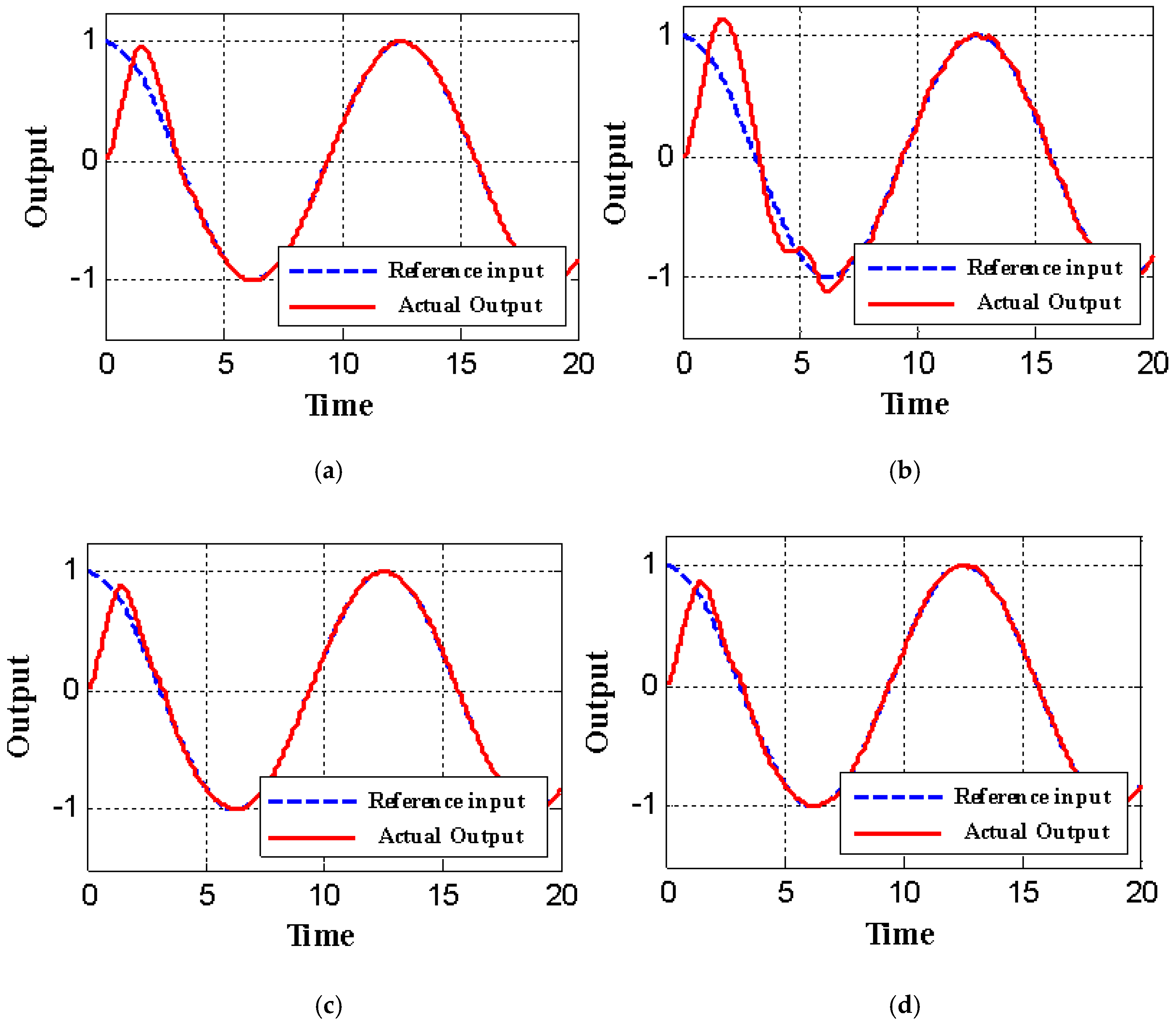
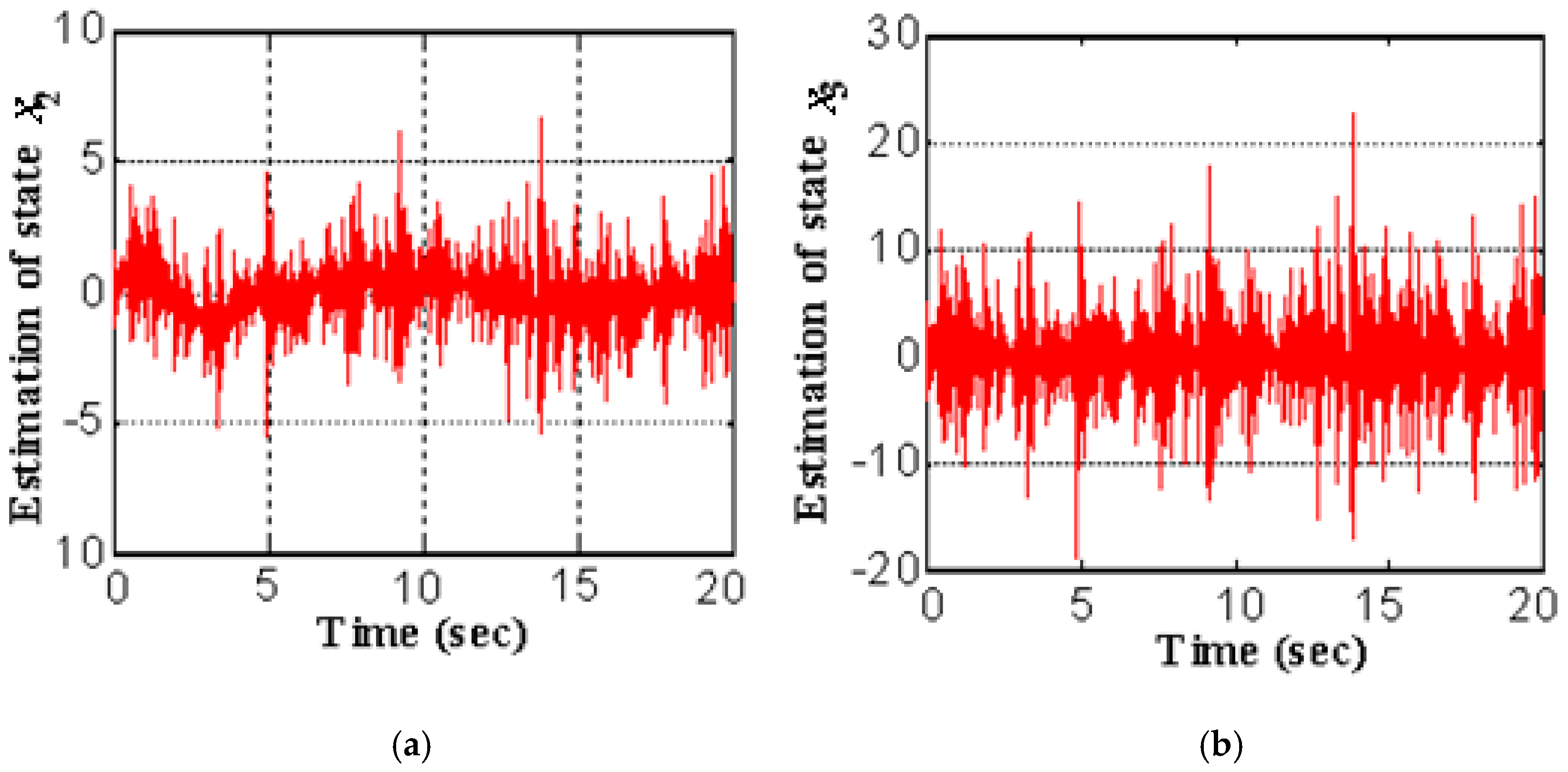
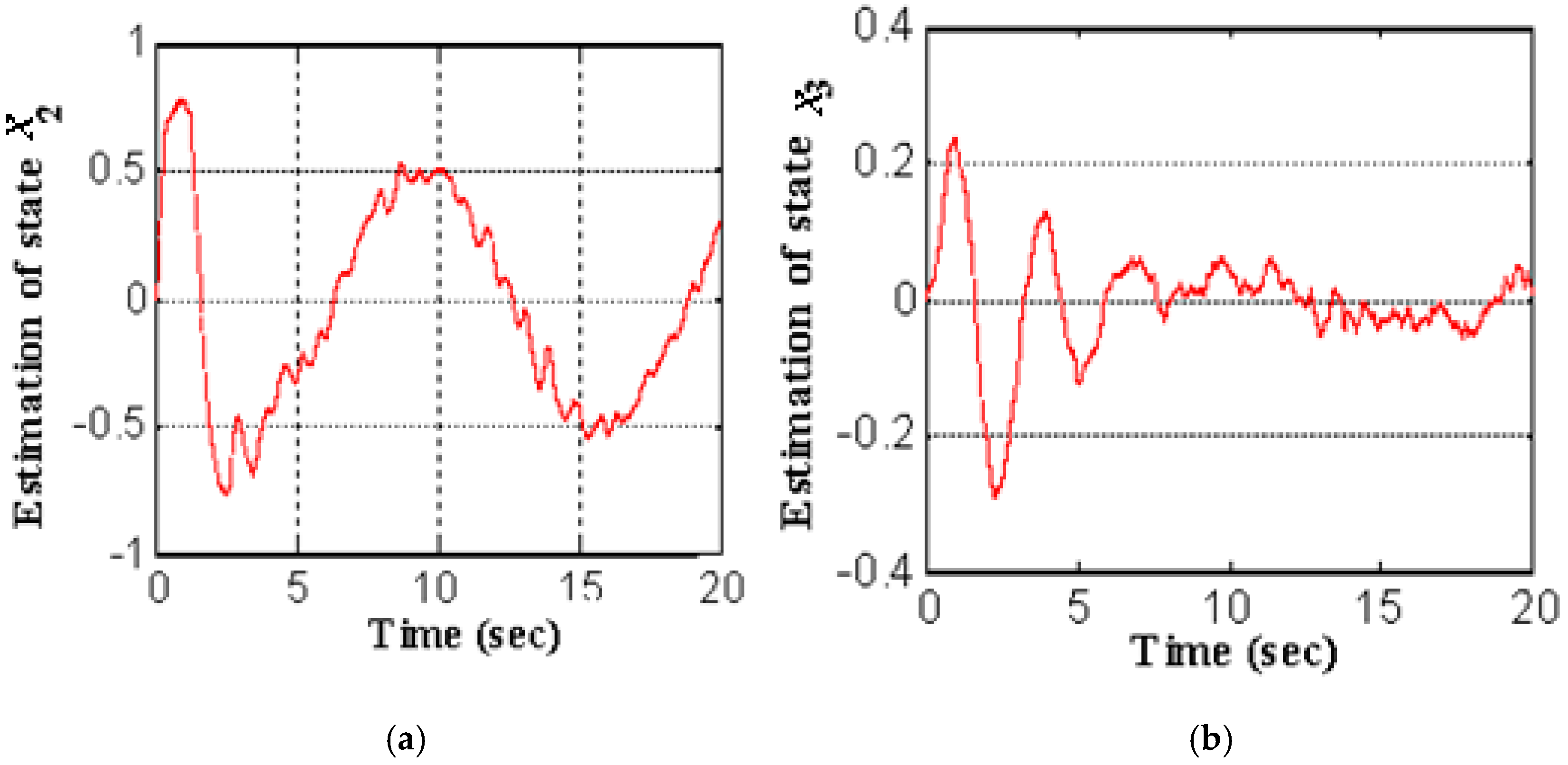
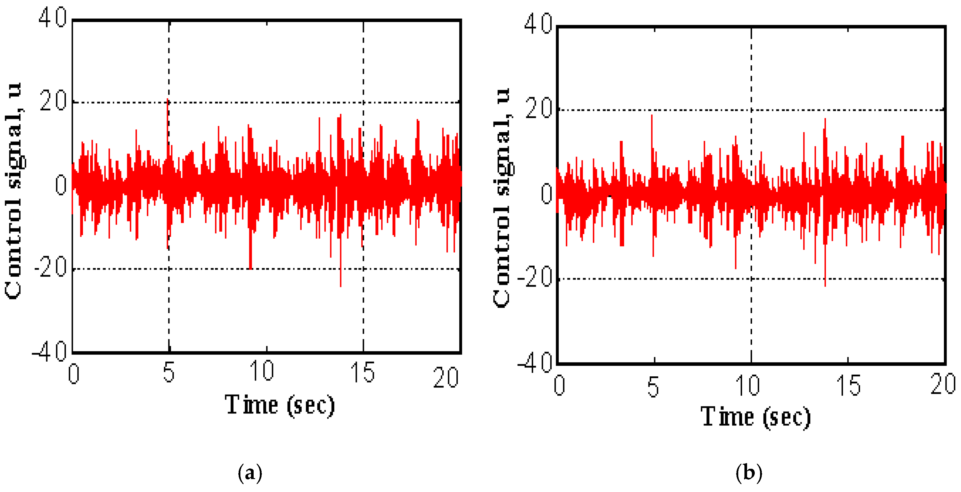
Both controllers and the suggested system were numerically simulated using MATLAB®/Simulink® ODE45 solver for models with continuous states. The reference input (r(t)) to the system was cos ( 0.5 t ) applied at t = 0 sec. Two test conditions were considered for this work. In the first case, the output of the proposed system did not include any measurement noise, while in the second test case, a Gaussian noise was applied with variance ( σ ) equal to 10 4 and the mean μ = 0 . The simulation results of both conventional ADRC and N-ADRC are shown in Figure 3. The estimated states x ^ 2 and x ^ 3 of the nonlinear system given in Equation (50) using C-ADRC scheme are shown in Figure 4. These states are also estimated using the N-ADRC scheme and are depicted in Figure 5. Moreover, the control signals for both schemes are illustrated in Figure 6.
As shown in Figure 3b, the presence of measurement noise has an adverse effect on the time response of the output for the in the case of C-ADRC, especially at the time interval [1.5,7] sec which shows large oscillations in the output response. The effect is not shown in the case of the N-ADRC (see Figure 3d).
The estimated states of the C-ADRC shown in Figure 4 were highly affected by the measurement noise included in the output opposite the case of utilizing the N-ADRC, in which the noise had negligible effect at the estimated state (refer to Figure 5). This behaviour on the control signal was illustrated in Figure 6. This due to the bandwidth ( ω 0 ) of the ESO in the C-ADRC is less than the bandwidth ( ω 0 ) for the outer ESO.
The numerical results are listed in Table 1. Adding measurement noise to the measured output significantly affected the output response—the Integral Time Absolute Error (ITAE)—and the total energy of the actuating signal (ISU) of the C-ADRC controller. In Table 1, ITAE = 0 20 t | y r | d t is the integration of the time absolute error for the output signal, and ISU = 0 20 u 2   d t is the integration of the square of the control signal.
It is worth mentioning that, in our simulation, we have set the bandwidth ( ω 0 ) of the ESO in the C-ADRC to 100 rad/sec, while, for our proposed structure, a bandwidth ( ω 0 ) for the inner ESO was set to 100 rad/sec, and a bandwidth ( ω 0 ) for the outer ESO had a value of 22.83 rad/sec. It is clear that a big reduction in the bandwidth requirements in our proposed structure achieved a noticeable improvement in the performance in terms of both ITAE and ISU, especially in the noisy case.
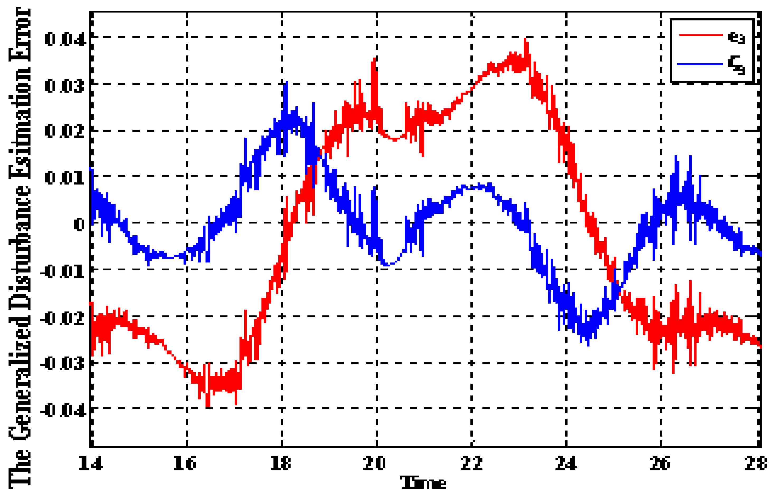
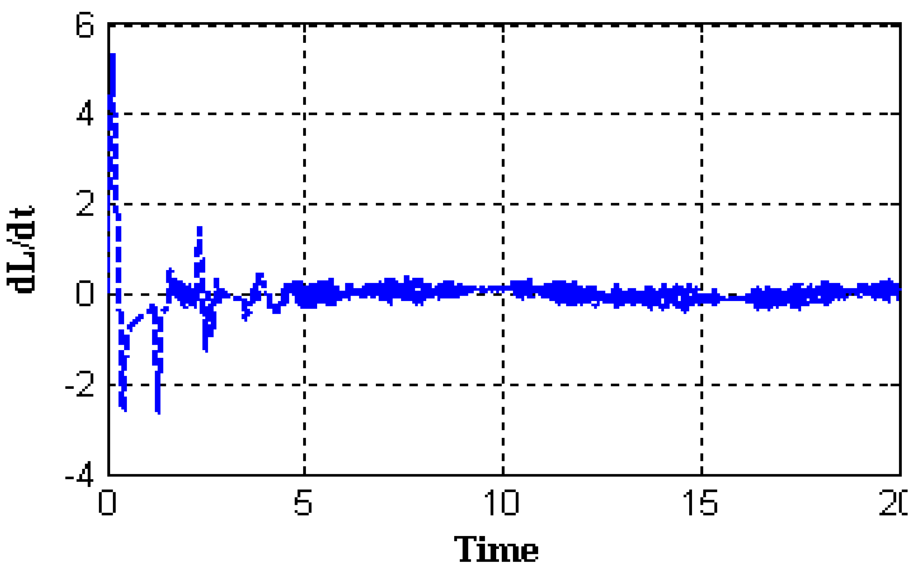
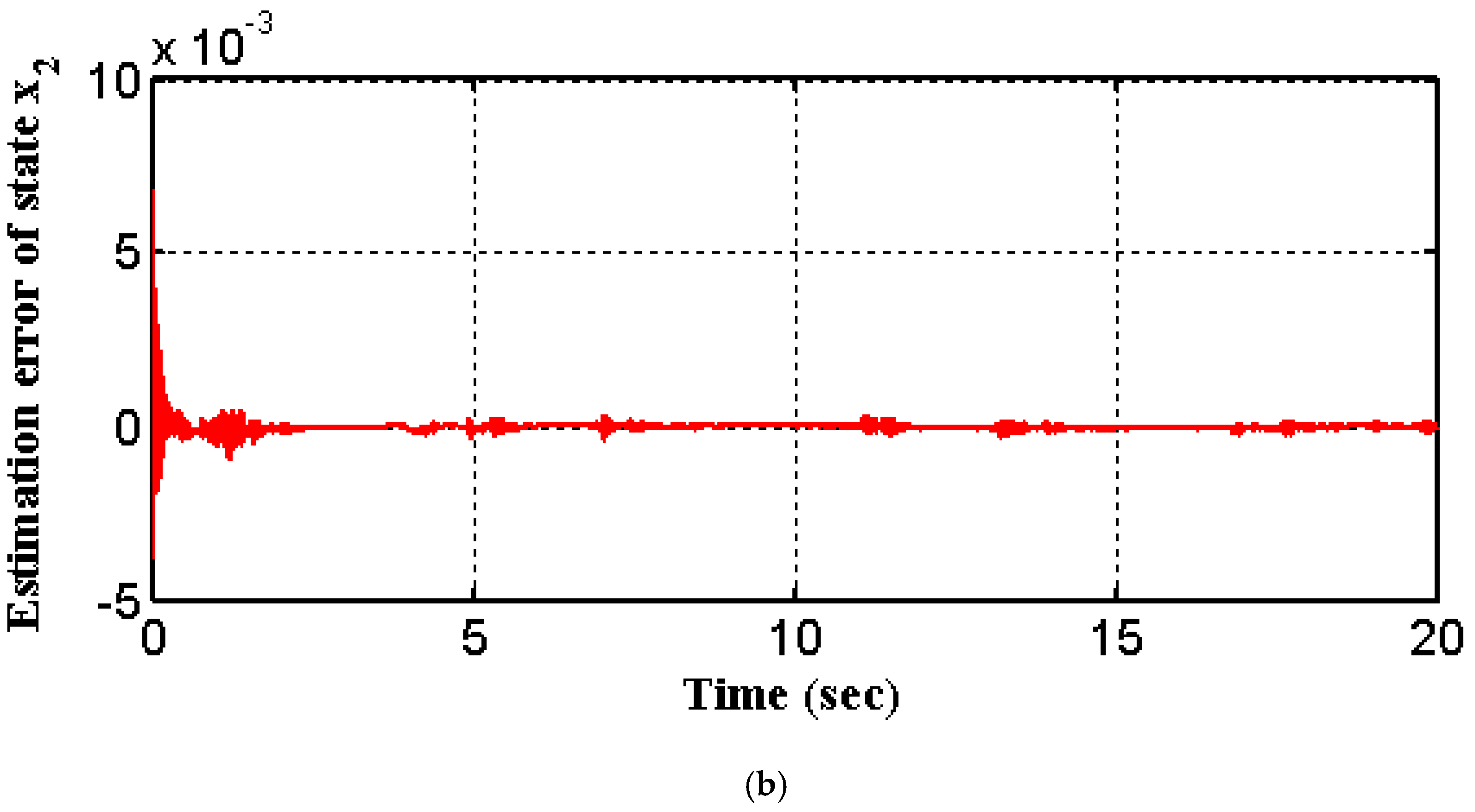
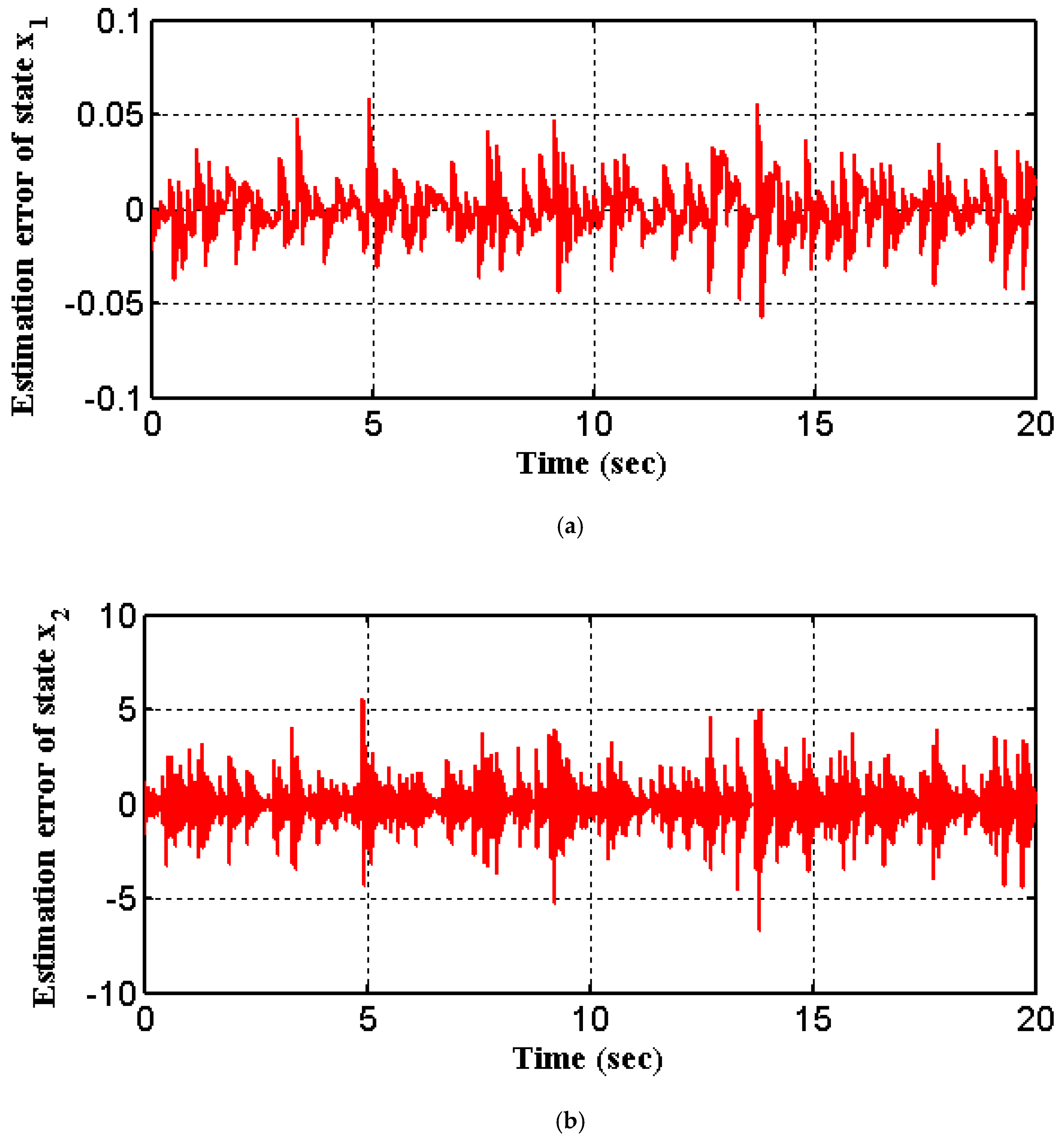
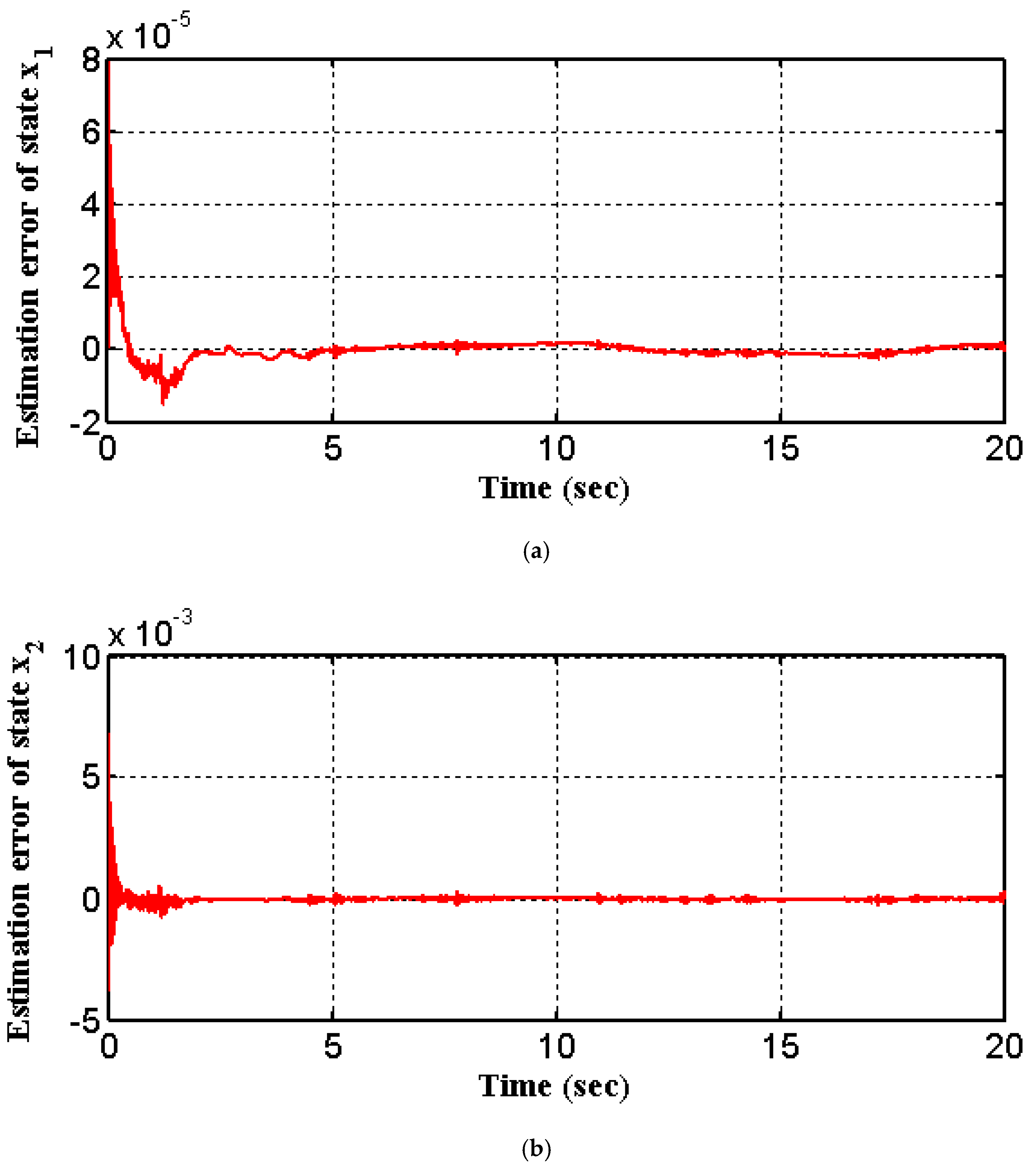
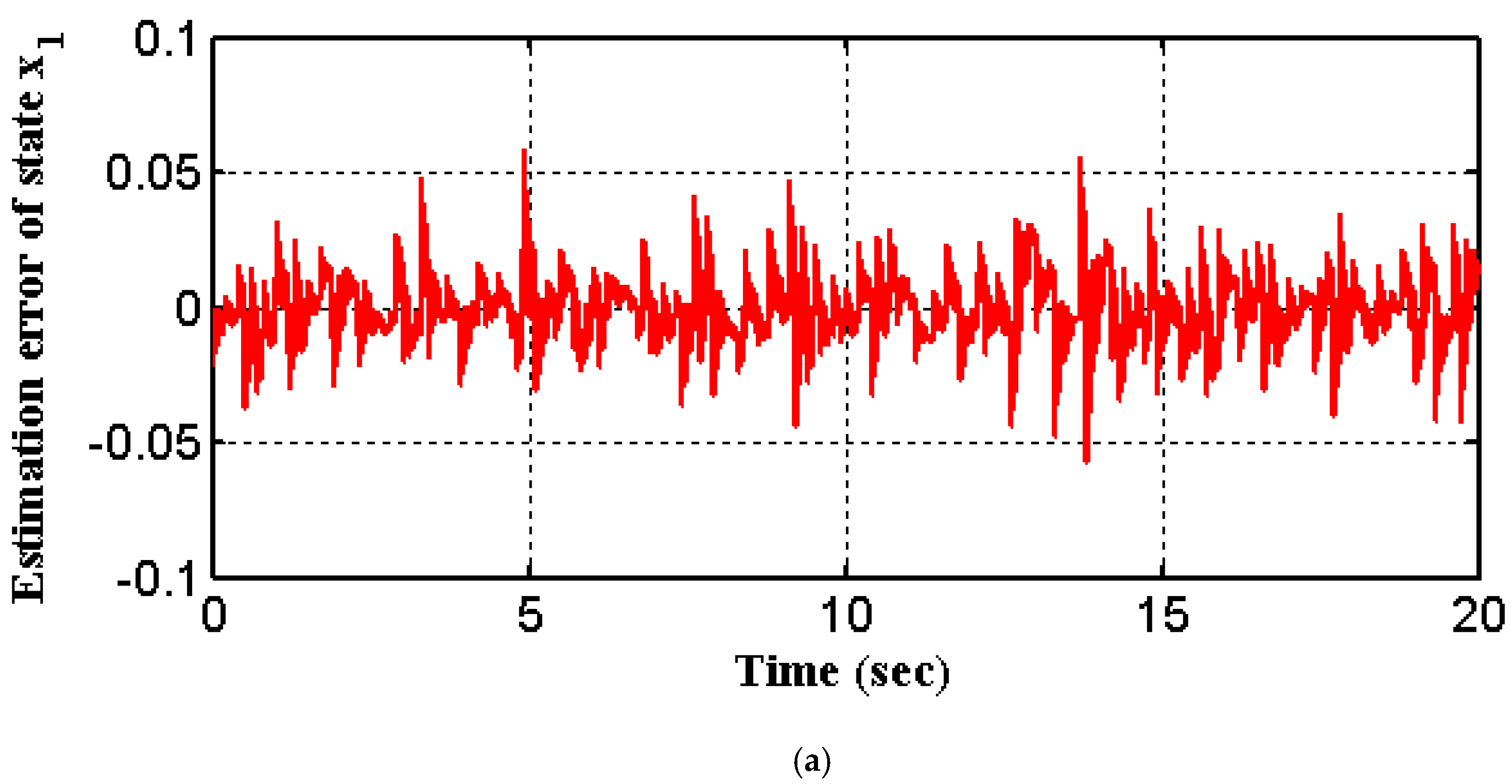
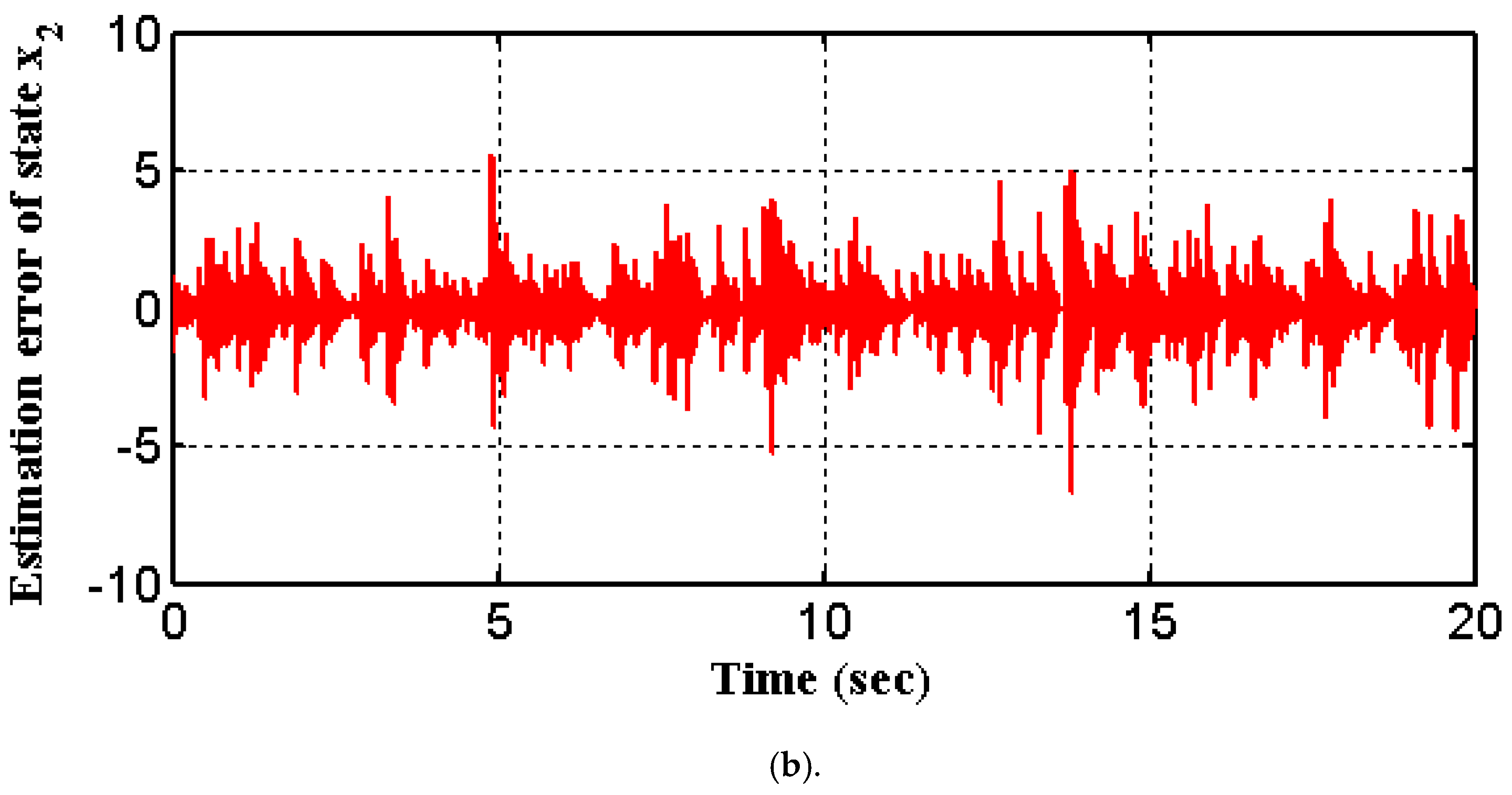
The estimation error of the generalized disturbances for the inner LESO is described by e 3 , which is given in Equation (12), and the generalized disturbance estimation error of the outer LESO is described by ζ 3 , which is given in Equation (32); both of these are illustrated in Figure 7. The ITAE of e 3 is 10.5769 and the ITAE of ζ 3 is 5.8251, displaying a percentage reduction in the ITAE equal to 45%. Figure 4 more clearly illustrates the reduction in ζ 3 against e 3 . As illustrated in Figure 8 the derivative of the generalized disturbance Δ ( t ) = d L d t is bounded during the transient period by 5.34 and at the steady state by 0.3. Assumption A1 is already satisfied. Moreover, the estimation errors of the C-ADRC with and without measurement noise are shown in Figure 9 and Figure 10, respectively. In the same manner, the estimation errors of the N-ADRC with and without measurement noise are shown in Figure 11 and Figure 12, respectively.

5.2. The Nonlinear Mass–Spring–Damper Model

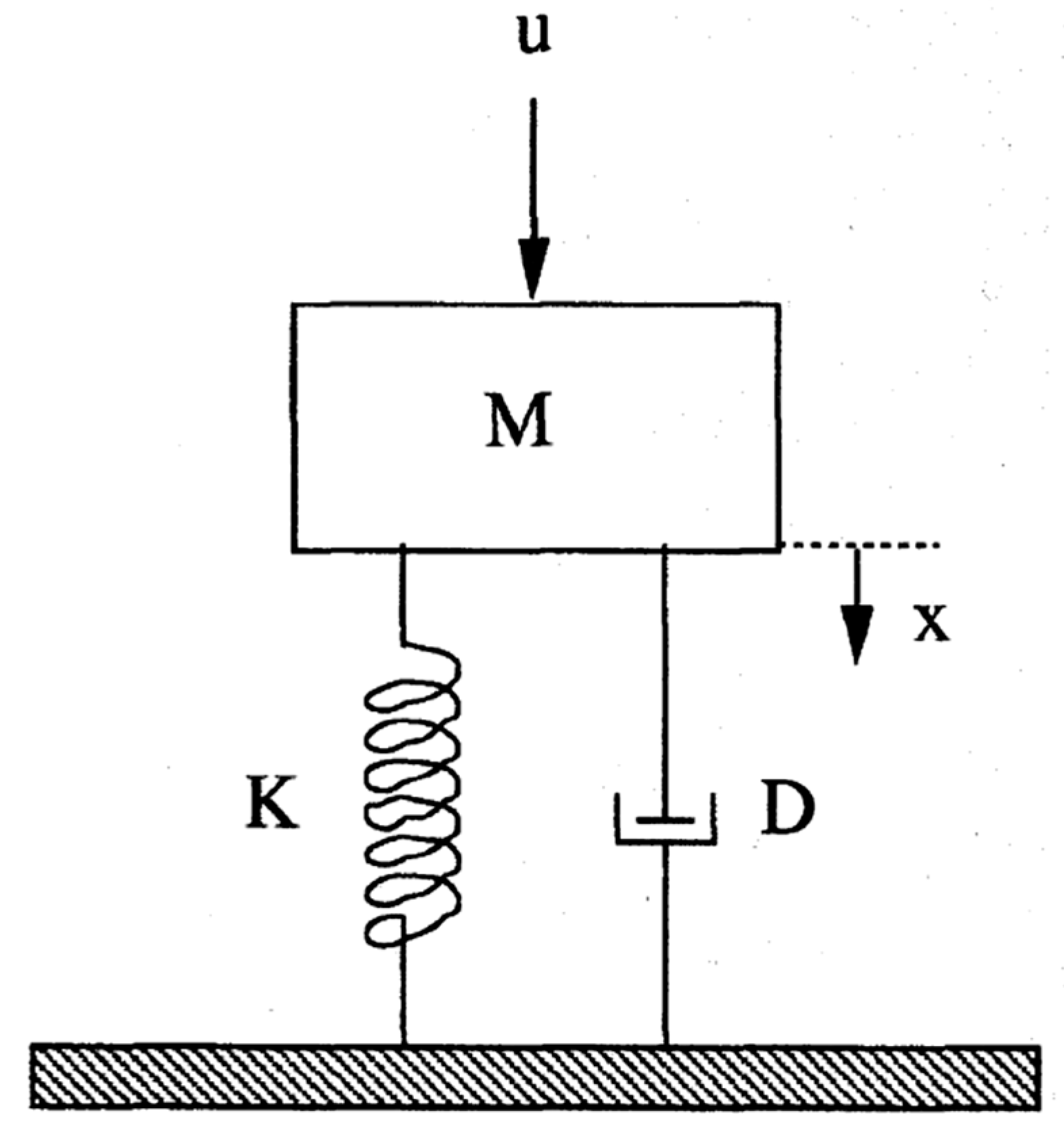
A simple nonlinear Mass–Spring–Damper (MSD) mechanical system is shown in Figure 13. It can be described as follows [44]:
M x ¨ + g ( x , x ˙ ) + f ( x ) = φ ( x ˙ ) u
where M is the mass and u is the input force, f ( x ) is the nonlinear or uncertain term with respect to the spring, g ( x , x ˙ )   is the nonlinear or uncertain term with respect to the damper, and φ ( x ˙ ) is the nonlinear term with respect to the input term. Let, g ( x , x ˙ ) = D ( d 1 x + d 2 x ˙ 3 ) ,   f ( x ) = d 3 x + d 4 x 3 , and φ ( x ˙ ) = 1 + d 5 x ˙ 3 , where x [ a   a ] ,   and   x ˙ [ b   b ] ,   a , b > 0 . The parameters are listed in Table 2.
Then, Equation (55) can be rewritten as follows:
x ¨ = 0.1 x ˙ 3 0.02 x 0.67 x 3 + u
The state-space representation of the nonlinear MSD model is expressed as:
{ x ˙ 1 = x 2 x ˙ 2 = 0.1 x 2 3 0.02   x 1 0.67   x 1 3 + u y = x 1
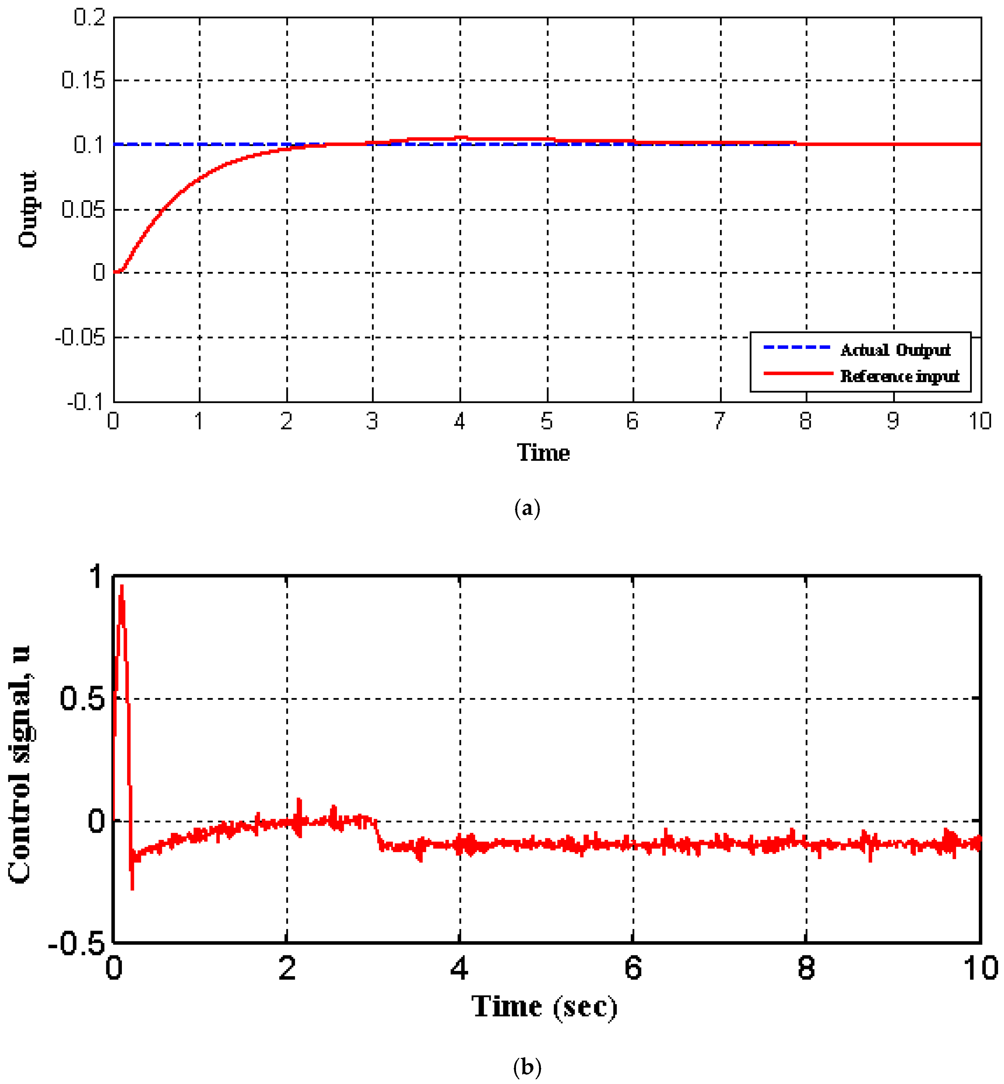
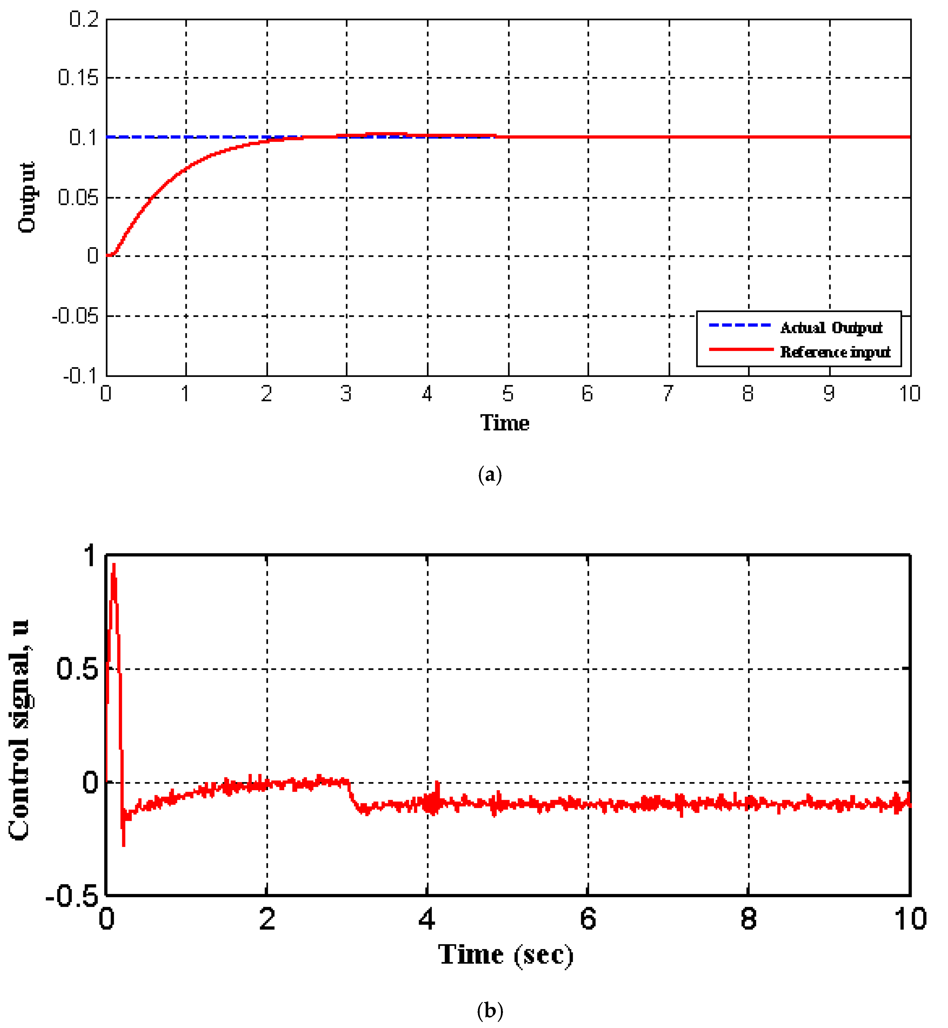
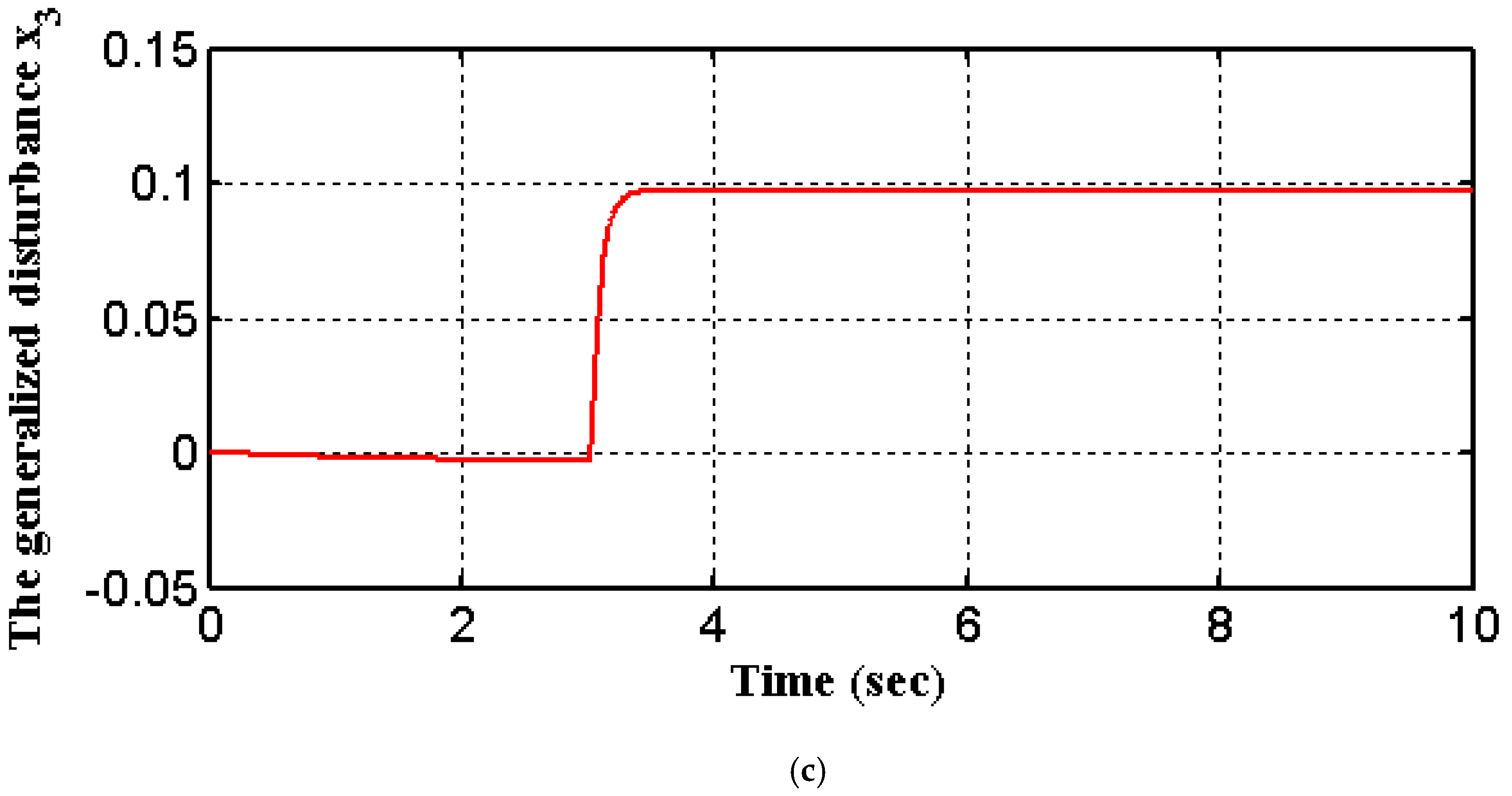
The results of the numerical simulation for the case of the nonlinear mass–spring–damper model using both the C-ADRC and the proposed N-ADRC are shown in Figure 14 and Figure 15, respectively.
The numerical results are listed in Table 3. Adding an extra LESO to the C-ADRC significantly affected the output response (ITAE) of the N-ADRC controller. In Table 3, ITAE = 0 20 t | y r | d t is the integration of the time absolute error for the output signal, and ISU = 0 20 u 2   d t is the integration of the square of the control signal.

6. Conclusions

This paper presented a novel approach to the design of a new class of LESO achieved by nesting an additional LESO in parallel with the original to obtain an N-ADRC. The proposed N-ADRC was successfully applied to the hypothetical SISO and a highly uncertain nonlinear SISO system with exogenous disturbance, as given in Equation (50). It can be concluded that the N-ADRC outperforms the C-ADRC in terms of control effort, output tracking, and disturbance rejection, as well as, more obviously, in the case of measurement error. In contrast with the C-ADRC, when the order of the LESO increases, the issue of measurement noise could be challenging, where increasing bandwidth is the only option for obtaining better performance, the main outcome of this work was to show that an outer-loop LESO connected in parallel with the inner-loop LESO removes the need to increase the bandwidth of the inner-loop LESO as has been shown through the numerical simulations of this work. Furthermore, the N-ADRC can converge to the states of the original system asymptotically. The N-ADRC reduced the ITAE dramatically for cases both with and without measurement noise. Due to its simplicity, N-ADRC is suitable to be implemented in real-time applications. In future work, this approach can be extended to nest more than two LESOs, and nonlinear ESOs could also be used and their performance investigated for multi-input-multi-output (MIMO) systems. Finally, several real-world nonlinear models can be used to show the performance of the N-ADRC as given in [45,46,47,48,49,50,51,52,53].

Author Contributions

Conceptualization, I.K.I., W.R.A.-A.; methodology, I.K.I, W.R.A.-A., A.T.A, and A.J.H.; Supervision, I.K.I., A.T.A.; Investigation, I.K.I., A.T.A., A.J.H.; software, W.R.A.-A., A.J.H.; validation, A.T.A., A.J.H.; formal analysis, I.K.I., W.R.A.-A., A.T.A., A.J.H.; resources, A.J.H.; writing—original draft preparation W.R.A.-A., I.K.I., A.J.H.; writing—review and editing, W.R.A.-A., I.K.I., A.T.A., A.J.H.; visualization, W.R.A.-A., I.K.I., A.T.A.; funding acquisition, A.T.A. All authors have read and agreed to the published version of the manuscript.

Funding

This study was supported and funded by Prince Sultan University, Riyadh, Saudi Arabia.

Acknowledgments

The authors would like to thank Prince Sultan University, Riyadh, Saudi Arabia for supporting and funding this work. Special acknowledgment to Robotics and Internet-of-Things Lab (RIOTU) at Prince Sultan University, Riyadh, SA. Also, the authors wish to acknowledge the editor and anonymous reviewers for their insightful comments, which have improved the quality of this publication.

Conflicts of Interest

The authors declare no conflict of interest.

References

  1. Yang, J.; Chen, W.H.; Li, S. Non-linear disturbance observer-based robust control for systems with mismatched disturbances/uncertainties. IET Control Theory Appl. 2011, 5, 2053–2062. [Google Scholar] [CrossRef] [Green Version]
  2. Han, J. From PID to active disturbance rejection control. IEEE Trans. Ind. Electron. 2009, 56, 900–906. [Google Scholar] [CrossRef]
  3. Wang, H.P.; Zheng, D.; Tian, Y. High pressure common rail injection system modeling and control. ISA Trans. 2016, 63, 265–273. [Google Scholar] [CrossRef]
  4. Li, S.; Wang, H.; Tian, Y.; Aitouch, A.; Klein, J. Direct power control of DFIG wind turbine systems based on an intelligent proportional-integral sliding mode control. ISA Trans. 2016, 64, 431–439. [Google Scholar] [CrossRef]
  5. Gao, Z.; Huang, Y.; Han, J. An alternative paradigm for control system design. In Proceedings of the 40th IEEE Conference on Decision and Control, Orlando, FL, USA, 4–7 December 2001; pp. 4578–4585. [Google Scholar]
  6. Sayem, A.H.M.; Cao, Z.; Man, Z. Model Free ESO-based Repetitive Control for Rejecting Periodic and Aperiodic Disturbances. IEEE Trans. Ind. Electron. 2017, 64, 3433–3441. [Google Scholar] [CrossRef]
  7. Li, G.; Xu, W.; Zhao, J.; Wang, S.; Li, B. Precise robust adaptive dynamic surface control of permanent magnet synchronous motor based on extended state observer. IET Sci. Meas. Technol. 2017, 11, 590–599. [Google Scholar] [CrossRef]
  8. Abdul-Adheem, W.R.; Ibraheem, I.K. An Improved Active Disturbance Rejection Control for a Differential Drive Mobile Robot with Mismatched Disturbances and Uncertainties. arXiv 2018, arXiv:1805.12170. [Google Scholar]
  9. Li, S.; Yang, J.; Chen, W.H.; Chen, X. Generalized extended state observer based control for systems with mismatched uncertainties. IEEE Trans. Ind. Electron. 2012, 59, 4792–4802. [Google Scholar] [CrossRef] [Green Version]
  10. Liu, H.; Li, S. Speed control for PMSM servo system using predictive functional control and extended state observer. IEEE Trans. Ind. Electron. 2012, 59, 1171–1183. [Google Scholar] [CrossRef]
  11. Zhu, Z.; Xia, Y.; Fu, M. Adaptive sliding mode control for attitude stabilization with actuator saturation. IEEE Trans. Ind. Electron. 2011, 58, 4898–4907. [Google Scholar] [CrossRef]
  12. Yang, J.; Su, J.; Li, S.; Yu, X. High-order mismatched disturbance compensation for motion control systems via a continuous dynamic sliding-mode approach. IEEE Trans. Ind. Inform. 2014, 10, 604–614. [Google Scholar] [CrossRef] [Green Version]
  13. Abdul-adheem, W.R.; Ibraheem, I.K. Improved Sliding Mode Nonlinear Extended State Observer based Active Disturbance Rejection Control for Uncertain Systems with Unknown Total Disturbance. Int. J. Adv. Comput. Sci. Appl. 2016, 7, 80–93. [Google Scholar]
  14. Pu, Z.; Yuan, R.; Yi, J.; Tan, X. A Class of Adaptive Extended State Observers for Nonlinear Disturbed Systems. IEEE Trans. Ind. Electron. 2015, 62, 5858–5869. [Google Scholar] [CrossRef]
  15. Zhiqiang, P.; Ruyi, Y.; Xiangmin, T.; Jianqiang, Y. Design and Analysis of Time-varying Extended State Observer. In Proceedings of the 34th Chinese Control Conferrence, Hangzhou, China, 28–30 July 2015; pp. 753–758. [Google Scholar]
  16. Zhang, X.; Wang, H.; Tian, Y.; Peyrodie, L.; Wang, X. Model-free based neural network control with time-delay estimation for lower extremity exoskeleton. Neurocomputing 2018, 272, 178–188. [Google Scholar] [CrossRef]
  17. Fliess, M.; Join, C. Model-free control and intelligent PID controllers: Towards a possible trivialization of nonlinear control? IFAC Proc. 2009, 15, 1531–1550. [Google Scholar] [CrossRef] [Green Version]
  18. Bakhshande, F.; Bach, R.; Söffker, D. Robust control of a hydraulic cylinder using an observer-based sliding mode control: Theoretical development and experimental validation. Control Eng. Pract. 2020, 95, 104272. [Google Scholar] [CrossRef]
  19. Bakhshande, F.; Söffker, D. Proportional-Integral-Observer-Based Backstepping Approach for Position Control of a Hydraulic Differential Cylinder System with Model Uncertainties and Disturbances. J. Dyn. Syst. Meas. Control Trans. ASME 2018, 140, 121006. [Google Scholar] [CrossRef]
  20. Li, J.; Xia, Y.; Qi, X.; Gao, Z. On the Necessity, Scheme, and Basis of the Linear-Nonlinear Switching in Active Disturbance Rejection Control. IEEE Trans. Ind. Electron. 2017, 64, 1425–1435. [Google Scholar] [CrossRef]
  21. Zheng, Q.; Gaol, L.Q.; Gao, Z. On stability analysis of active disturbance rejection control for nonlinear time-varying plants with unknown dynamics. In Proceedings of the 46th Annual Conference on Decision and Control, New Orleans, LA, USA, 12–14 December 2007; pp. 3501–3506. [Google Scholar]
  22. Farza, M.; Hern, O.; Saad, M.M.; Cedex, C. Cascade predictors design for a class of nonlinear uncertain systems with delayed state- Application to bioreactor. In Proceedings of the 17th International Conference on Automatic Control and Computer Engineering, Sousse, Tunisia, 19–21 November 2016; pp. 753–760. [Google Scholar]
  23. Vasconcelos, J.F.; Silvestre, C.; Oliveira, P. Pose Observers for Unmanned Air Vehicles. In Proceedings of the European Control Conference (ECC), Budapest, Hungary, 23–26 August 2009; pp. 3989–3994. [Google Scholar]
  24. Jiang, P.; Hao, J.Y.; Zong, X.P.; Wang, P.G. Modeling and simulation of Active-Disturbance-Rejection Controller with Simulink. In Proceedings of the 2010 International Conference on Machine Learning and Cybernetics ICMLC, Qingdao, China, 11–14 July 2010; pp. 927–931. [Google Scholar]
  25. Parvathy, R.; Daniel, A.E. A survey on active disturbance rejection control. In Proceedings of the 2013 International Multi Conference on Automation, Computing, Control, Communication and Compressed Sensing, Kottayam, India, 22–23 March 2013; pp. 330–335. [Google Scholar]
  26. Nowicki, M.; Madoński, R.; Kozłowski, K. First look at conditions on applicability of ADRC. In Proceedings of the 10th International Workshop on Robot Motion and Control (RoMoCo), Poznan, Poland, 6–8 July 2015; pp. 294–299. [Google Scholar]
  27. Al-Kalbani, F.; Al Hosni, S.M.; Zhang, J. Active Disturbance Rejection Control of a methanol-water separation distillation column. In Proceedings of the 2015 IEEE 8th GCC Conference Exhibition, Muscat, Oman, 1–4 February 2015; pp. 1–6. [Google Scholar]
  28. Lin, H.; Wang, X. Design and analysis of a continuous hybrid differentiator. IET Control Theory Appl. 2011, 5, 1321–1334. [Google Scholar]
  29. Wang, X.; Shirinzadeh, B. Rapid-convergent nonlinear differentiator. Mech. Syst. Signal Process. 2012, 28, 414–431. [Google Scholar] [CrossRef] [Green Version]
  30. Angulo, M.T.; Moreno, J.A.; Fridman, L. Robust exact uniformly convergent arbitrary order differentiator. Automatica 2013, 49, 2489–2495. [Google Scholar] [CrossRef]
  31. Ibraheem, I.K.; Abdul-adheem, W.R. On the Improved Nonlinear Tracking Differentiator based Nonlinear PID Controller Design. Int. J. Adv. Comput. Sci. Appl. 2016, 7, 234–241. [Google Scholar]
  32. Abdul-adheem, W.R.; Ibraheem, K. From PID to Nonlinear State Error Feedback Controller. Int. J. Adv. Comput. Sci. Appl. 2017, 8, 312–322. [Google Scholar]
  33. Kang, Y.L.; Shresta, G.B.; Lie, T.T. Application of an NLPID controller on a UPFC to improve transient stability of a power system. IEE Proc. Gener. Transm. Distrib. 2001, 148, 523–529. [Google Scholar] [CrossRef]
  34. Ma, L.; Lin, F.; You, X.; Zheng, T.Q. Nonlinear PID Control of Three-Phase Pulse Width Modulation Rectifier. In Proceedings of the 7th World Congress on Intelligent Control and Automation, Chongqing, China, 25–27 June 2008; pp. 3417–3422. [Google Scholar]
  35. Salim, S.N.S.; Ismail, Z.H.; Rahmat, M.F.; Faudzi, A.A.M.; Sunar, N.H.; Samsudin, S.I. Tracking performance and disturbance rejection of pneumatic actuator system. In Proceedings of the 9th Asian Control Conference, Istanbul, Turkey, 23–26 June 2013; pp. 1–6. [Google Scholar]
  36. Luenberger, D.G. Observing the State of a Linear System. IEEE Trans. Mil. Electron. 1964, 8, 74–80. [Google Scholar] [CrossRef]
  37. Goel, A.; Swarup, A. Performance Analysis of Active Disturbance Rejection Controlled Robotic Manipulator based on Evolutionary Algorithm. Int. J. Hybrid Inf. Technol. 2016, 9, 65–80. [Google Scholar] [CrossRef]
  38. Bao, D.; Tang, W. Adaptive sliding mode control of ball screw drive system with extended state observer. In Proceedings of the 2016 2nd International Conference on Control, Automation and Robotics ICCAR, Hong Kong, China, 28–29 April 2016; pp. 133–138. [Google Scholar]
  39. Godbole, A.A.; Kolhe, J.P.; Talole, S.E. Performance analysis of generalized extended state observer in tackling sinusoidal disturbances. IEEE Trans. Control Syst. Technol. 2013, 21, 2212–2223. [Google Scholar] [CrossRef]
  40. Pan, H.; Sun, W.; Gao, H.; Hayat, T.; Alsaadi, F. Nonlinear tracking control based on extended state observer for vehicle active suspensions with performance constraints. Mechatronics 2015, 30, 363–370. [Google Scholar] [CrossRef]
  41. Guo, B.Z.; Zhao, Z.L. On the convergence of an extended state observer for nonlinear systems with uncertainty. Syst. Control Lett. 2011, 60, 420–430. [Google Scholar] [CrossRef]
  42. Li, Y.; Yang, B.; Zheng, T.; Li, Y.; Cui, M.; Peeta, S. Extended-State-Observer-Based Double-Loop Integral Sliding-Mode Control of Electronic Throttle Valve. IEEE Trans. Intell. Transp. Syst. 2015, 16, 2501–2510. [Google Scholar] [CrossRef]
  43. Ball, A.A.; Khalil, H.K. High-gain observers in the presence of measurement noise: A nonlinear gain approach. In Proceedings of the 47th IEEE Conference on Decision and Control, Cancun, Mexico, 9–11 Dcember 2008; pp. 2288–2293. [Google Scholar]
  44. Xiu, Z.; Wang, W. A Novel Nonlinear PID Controller Designed By Takagi-Sugeno Fuzzy Model. In Proceedings of the 2006 6th World Congress on Intelligent Control and Automation, Dalian, China, 21–23 June 2006; pp. 3724–3728. [Google Scholar]
  45. Ibraheem, I.K. A Digital-Based Optimal AVR Design of Synchronous Generator Exciter using LQR Technique. Al-Khwarizmi Eng. J. 2011, 7, 82–94. [Google Scholar]
  46. Mohammed, I.A.; Mahir, R.A.; Ibraheem, I.K. Robust Controller Design for Load Frequency Control in Power Systems using State-Space Approach. J. Eng. Coll. Eng. Baghdad Univ. 2011, 17, 265–278. [Google Scholar]
  47. Ibraheem, I.K. Design of a two-Degree-of-Freedom Controller for a Magnetic Levitation System Based on LQG Technique. Al-Nahrain Eng. J. College Eng. Al-Nahrain Univ. 2013, 16, 67–77. [Google Scholar]
  48. Ibraheem, I.K.; Ajeil, F.H. Path Planning of an autonomous Mobile Robot using Swarm based Optimization Techniques. Al-KAwarizmi Eng. J. 2016, 12, 12–25. [Google Scholar] [CrossRef]
  49. Ibraheem, I.K. Anti-Disturbance Compensator Design for Unmanned Aerial Vehicle. J. Eng. 2020, 26, 86–103. [Google Scholar] [CrossRef] [Green Version]
  50. Abdul-Adheem, W.R.; Ibraheem, I.K.; Azar, A.T.; Humaidi, A.J. Improved Active Disturbance Rejection-Based Decentralized control for MIMO Nonlinear Systems: Comparison with The Decoupled Control Scheme. Appl. Sci. 2020, 10, 2515. [Google Scholar] [CrossRef] [Green Version]
  51. Ajeil, F.H.; Ibraheem, I.K.; Azar, A.T.; Humaidi, A.J. Grid-Based Mobile Robot Path Planning Using Aging-Based Ant Colony Optimization Algorithm in Static and Dynamic Environments. Sensors 2020, 20, 1880. [Google Scholar] [CrossRef] [Green Version]
  52. Ibraheem, G.A.R.; Azar, A.T.; Ibraheem, I.K.; Humaidi, A.J. A Novel Design of a Neural Network based Fractional PID Controller for Mobile Robots Using Hybridized Fruit Fly and Particle Swarm Optimization. Complexity 2020. [Google Scholar] [CrossRef]
  53. Bucolo, M.; Buscarino, A.; Famoso, C.; Fortuna, L.; Frasca, M. Control of imperfect dynamical systems. Nonlinear Dyn. 2019, 98, 2989–2999. [Google Scholar] [CrossRef]
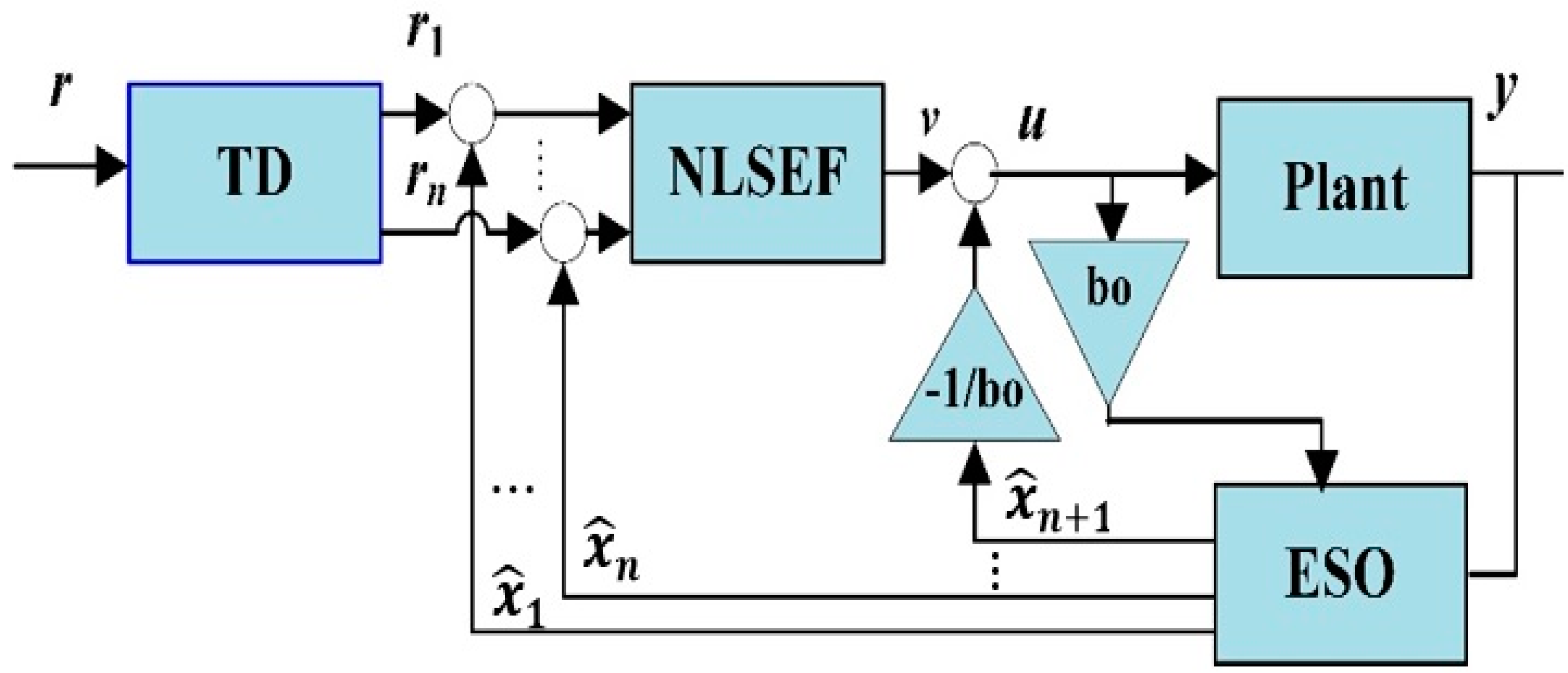
Figure 1. Structure of conventional Active Disturbance Rejection Control (ADRC).
Applsci 10 04069 g001
Figure 2. The Novel Active Disturbance Rejection Control (N-ADRC) structure with nested Linear Extended State Observers (LESOs).
Applsci 10 04069 g002
Figure 3. The output response curves (y). (a) Conventional ADRC (C-ADRC) (without measurement noise), (b) C-ADRC (with measurement noise), (c) N-ADRC (without measurement noise), (d) N- ADRC (with measurement noise).
Applsci 10 04069 g003
Figure 4. Estimated states using C-ADRC with measurement noise, (a) x ^ 2 , (b) x ^ 3 .
Applsci 10 04069 g004
Figure 5. Estimated states using outer-loop LESO for the N-ADRC with measurement noise, (a) z ^ 2 , (b) z ^ 3 .
Applsci 10 04069 g005
Figure 6. Control signals with measurement noise: (a) C-ADRC, (b) N-ADRC.
Applsci 10 04069 g006
Figure 7. The estimation errors of the generalized disturbances.
Applsci 10 04069 g007
Figure 8. The derivative of the generalized disturbance.
Applsci 10 04069 g008
Figure 9. Estimation errors without measurement noise using C-ADRC, (a) e 1 (b) e 2 .
Applsci 10 04069 g009aApplsci 10 04069 g009b
Figure 10. Estimation errors with measurement noise using C-ADRC, (a) e 1 (b) e 2 .
Applsci 10 04069 g010
Figure 11. Estimation error without measurement noise using N-ADRC, (a) e 1 (b) e 2 .
Applsci 10 04069 g011
Figure 12. Estimation error with measurement noise using N-ADRC, (a) e 1 (b) e 2 .
Applsci 10 04069 g012aApplsci 10 04069 g012b
Figure 13. The nonlinear mass–spring–damper model.
Applsci 10 04069 g013
Figure 14. The results for the mass spring dumper model using C-ADRC, (a) output (y), (b) control signal (u), (c) the generalized disturbance.
Applsci 10 04069 g014aApplsci 10 04069 g014b
Figure 15. The result for the mass spring dumper model using N-ADRC, (a) output (y), (b) control signal, (c) the generalized disturbance.
Applsci 10 04069 g015aApplsci 10 04069 g015b
Table 1. Performance indices.
SymbolWithout NoiseWith Noise
ITAEISUITAEISU
C-ADRC1.717.177.07457.30
N-ADRC1.336.632.13310.91
Reduction (%)22.327.5169.8732.01
Table 2. Model parameters.
ParameterValue
M 1.0
D 1.0
d 1 0.01
d 2 0.1
d 3 0.01
d 4 0.67
d 5 0
a 1.5
b 1.5
Table 3. Performance indices.
ControllerITAEISU
C-ADRC0.100.17
N-ADRC0.050.16
Reduction (%)506