Figure 1.
Structure and winding pattern of the stator.
Figure 1.
Structure and winding pattern of the stator.
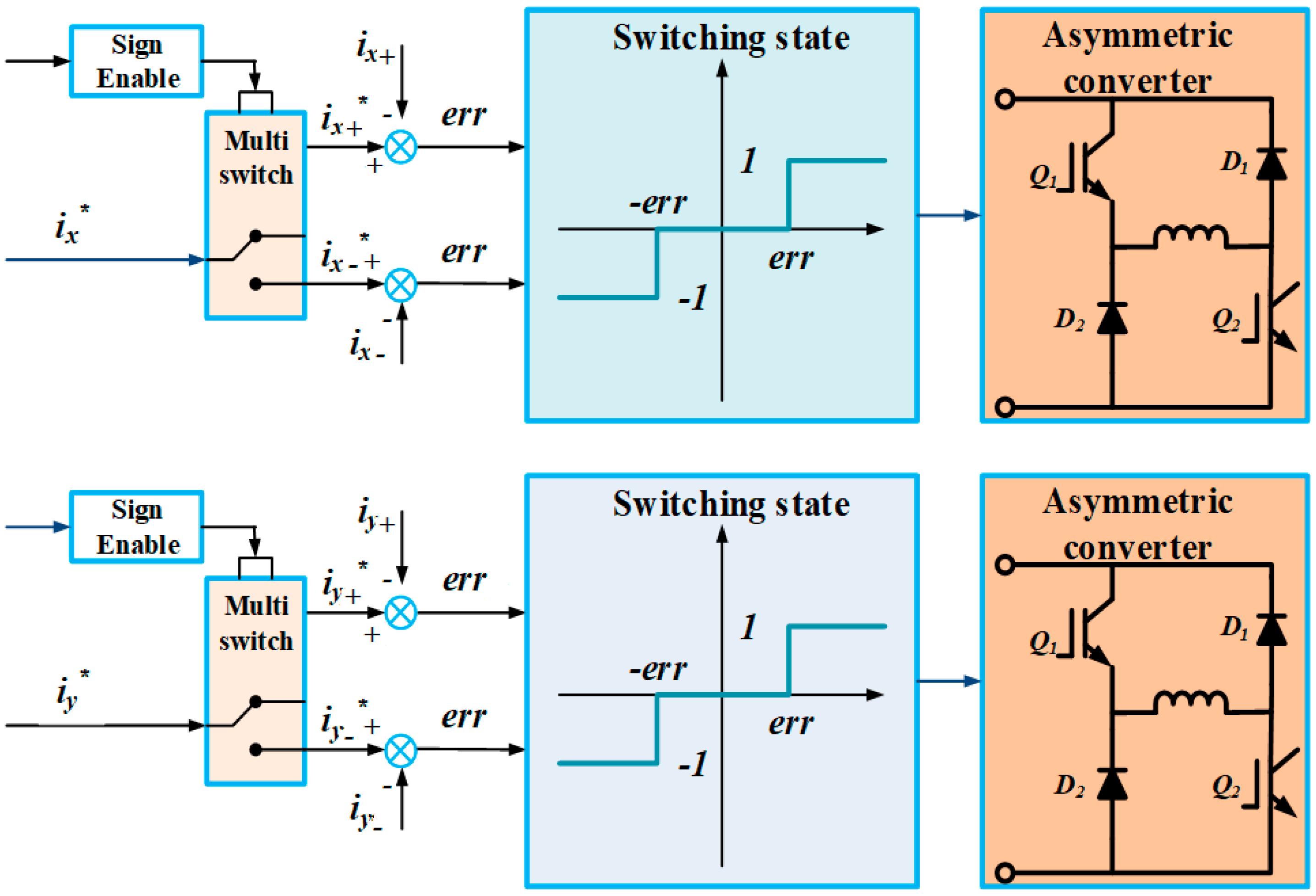
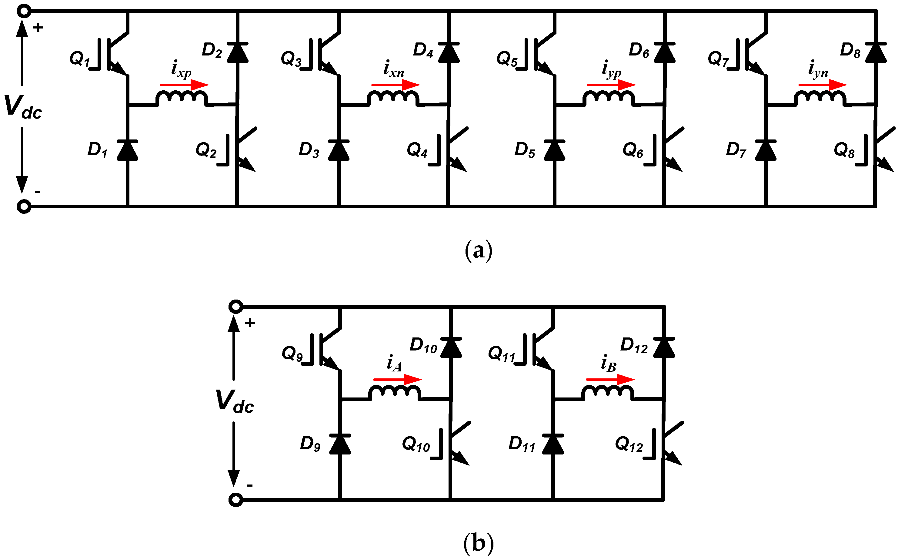
Figure 2.
Switching states of the hysteresis control method.
Figure 2.
Switching states of the hysteresis control method.
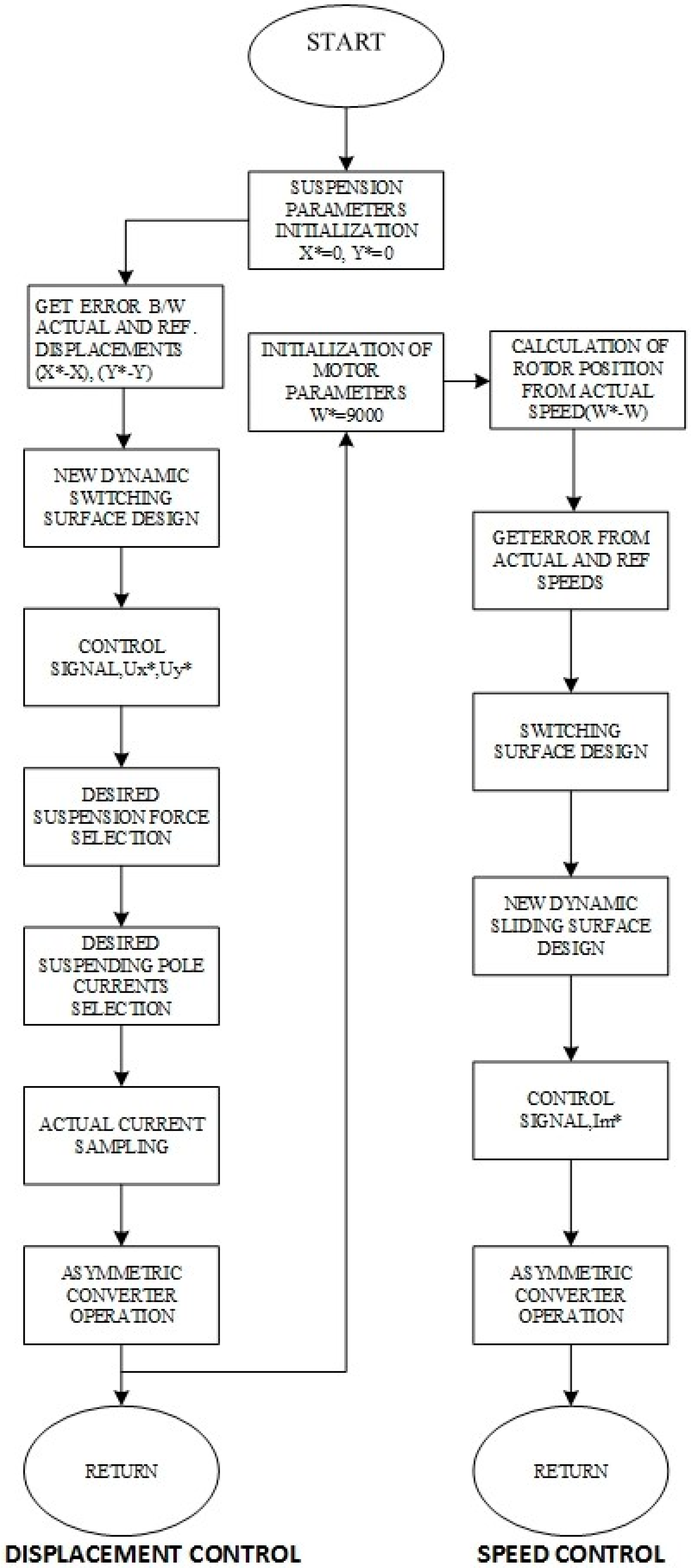
Figure 3.
Stepwise flow chart for the implementation of the dynamic sliding mode control of the bearingless switched reluctance motor (BSRM).
Figure 3.
Stepwise flow chart for the implementation of the dynamic sliding mode control of the bearingless switched reluctance motor (BSRM).
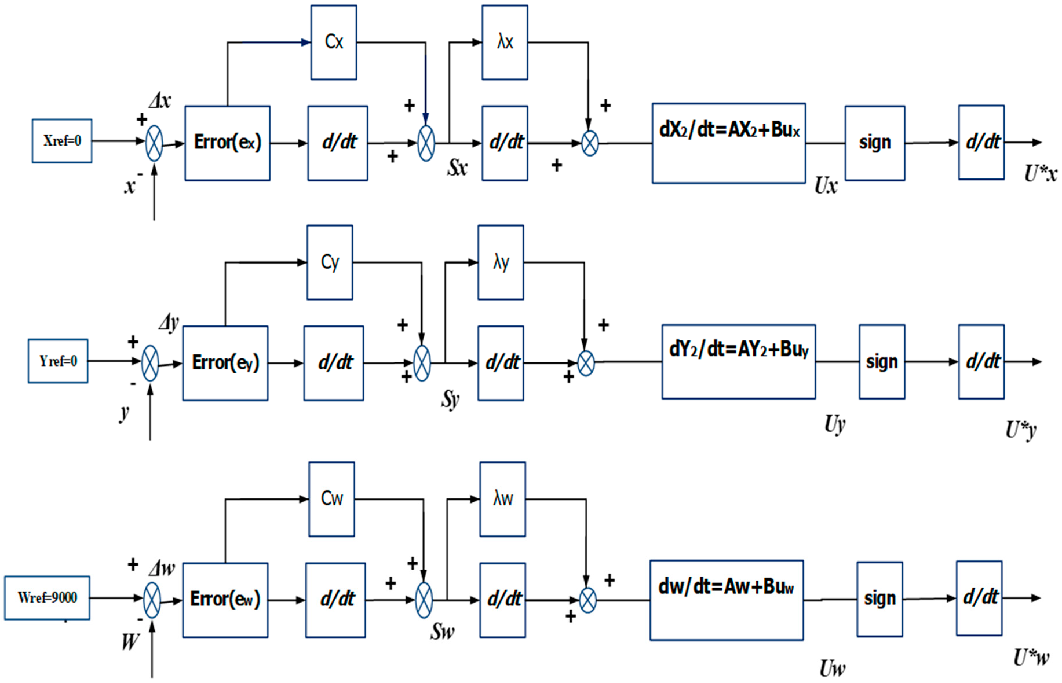
Figure 4.
Block diagram of the dynamic sliding mode control.
Figure 4.
Block diagram of the dynamic sliding mode control.
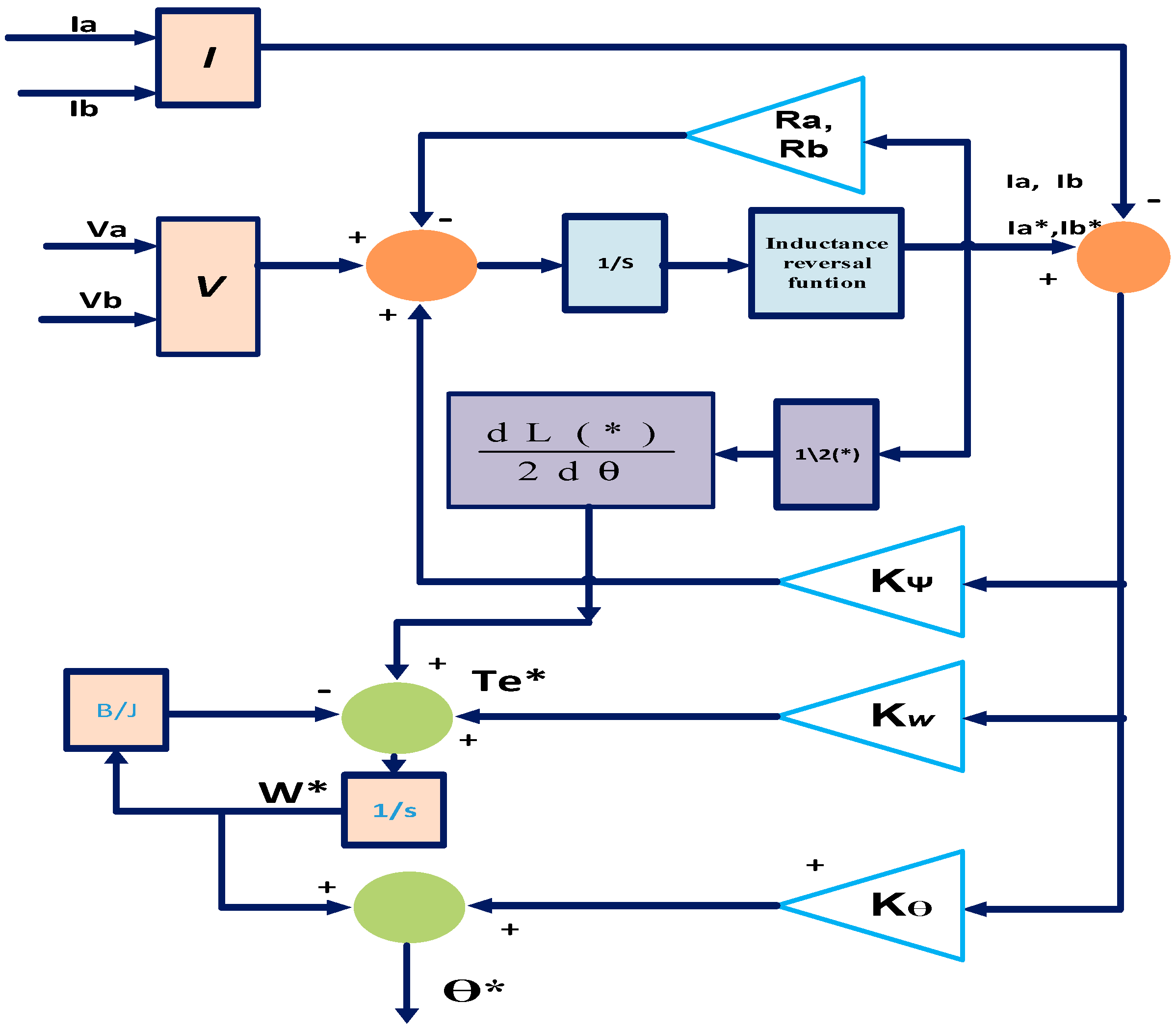
Figure 5.
Block diagram of the sliding mode observer.
Figure 5.
Block diagram of the sliding mode observer.
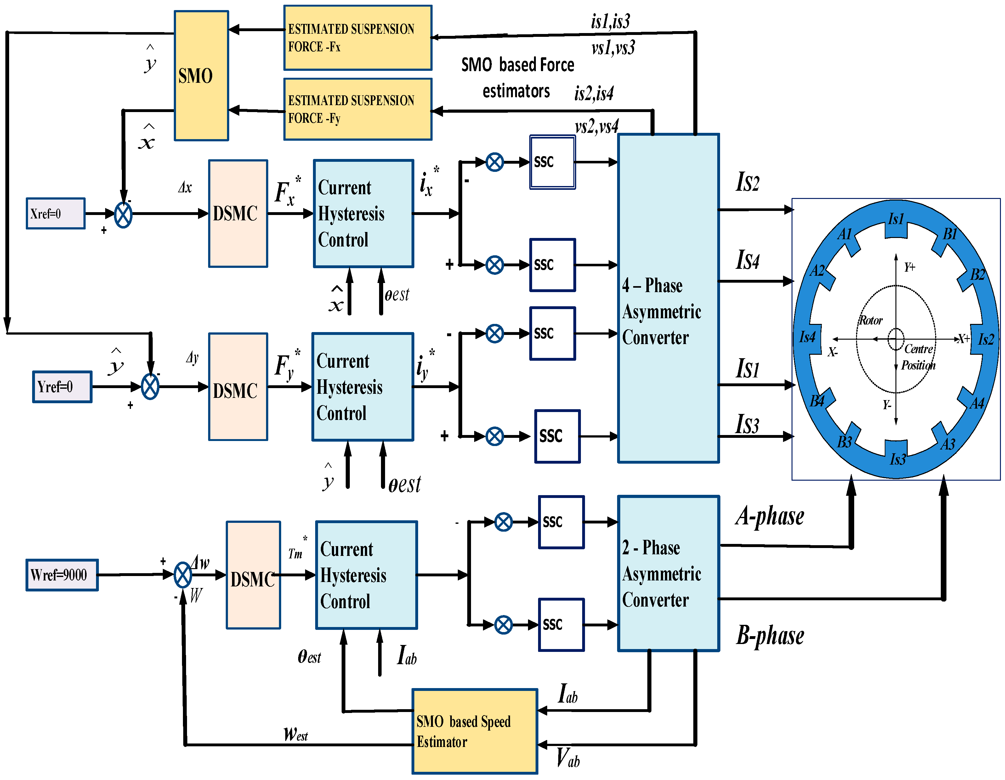
Figure 6.
Overall sensorless control block diagram of the BSRM.
Figure 6.
Overall sensorless control block diagram of the BSRM.
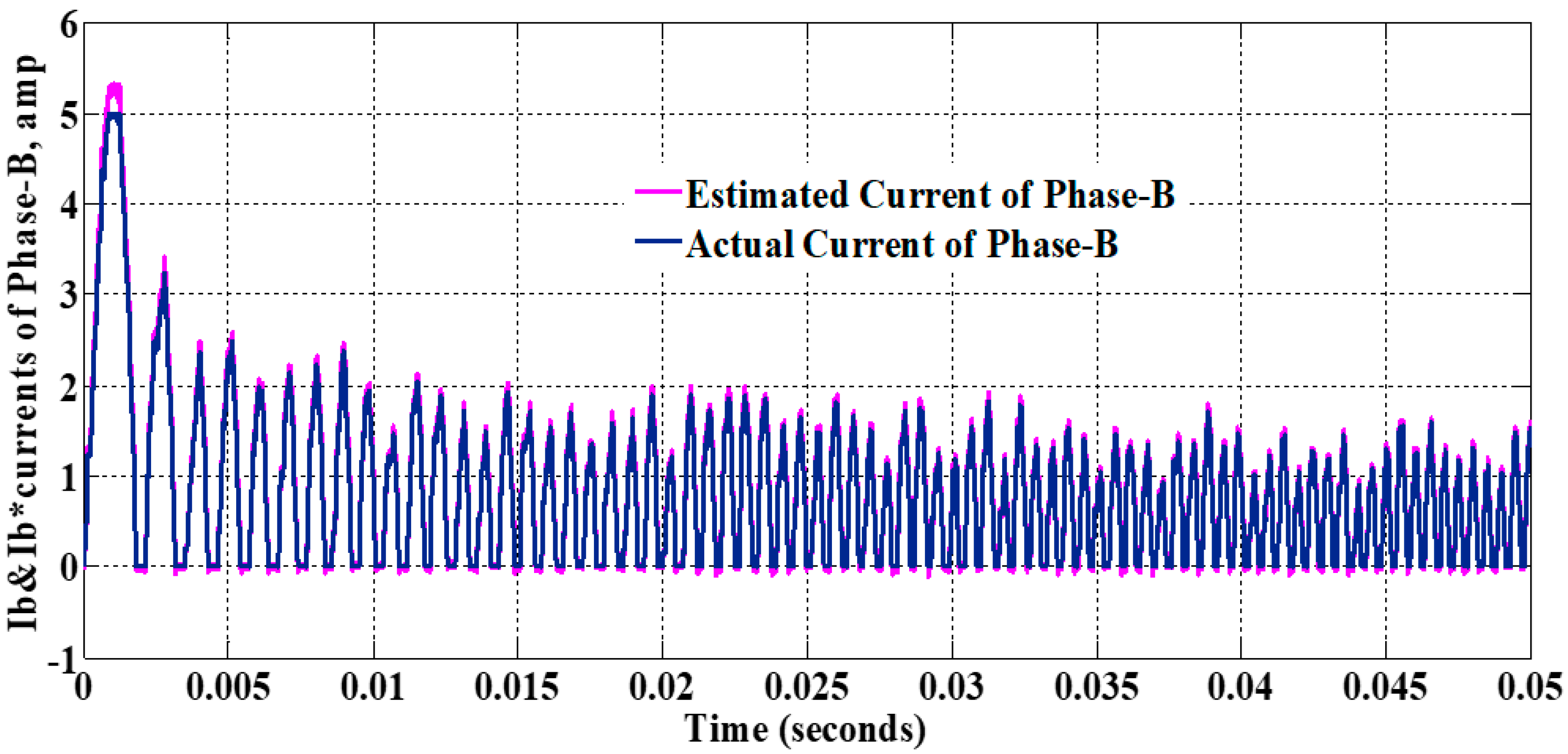
Figure 7.
Estimated and actual phase-B currents.
Figure 7.
Estimated and actual phase-B currents.
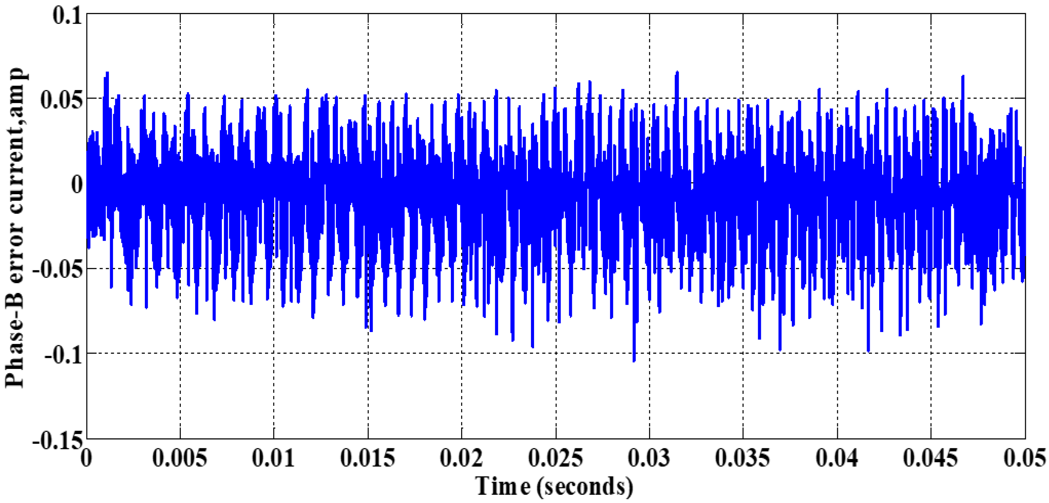
Figure 8.
Error between the estimated and actual currents of phase-B.
Figure 8.
Error between the estimated and actual currents of phase-B.
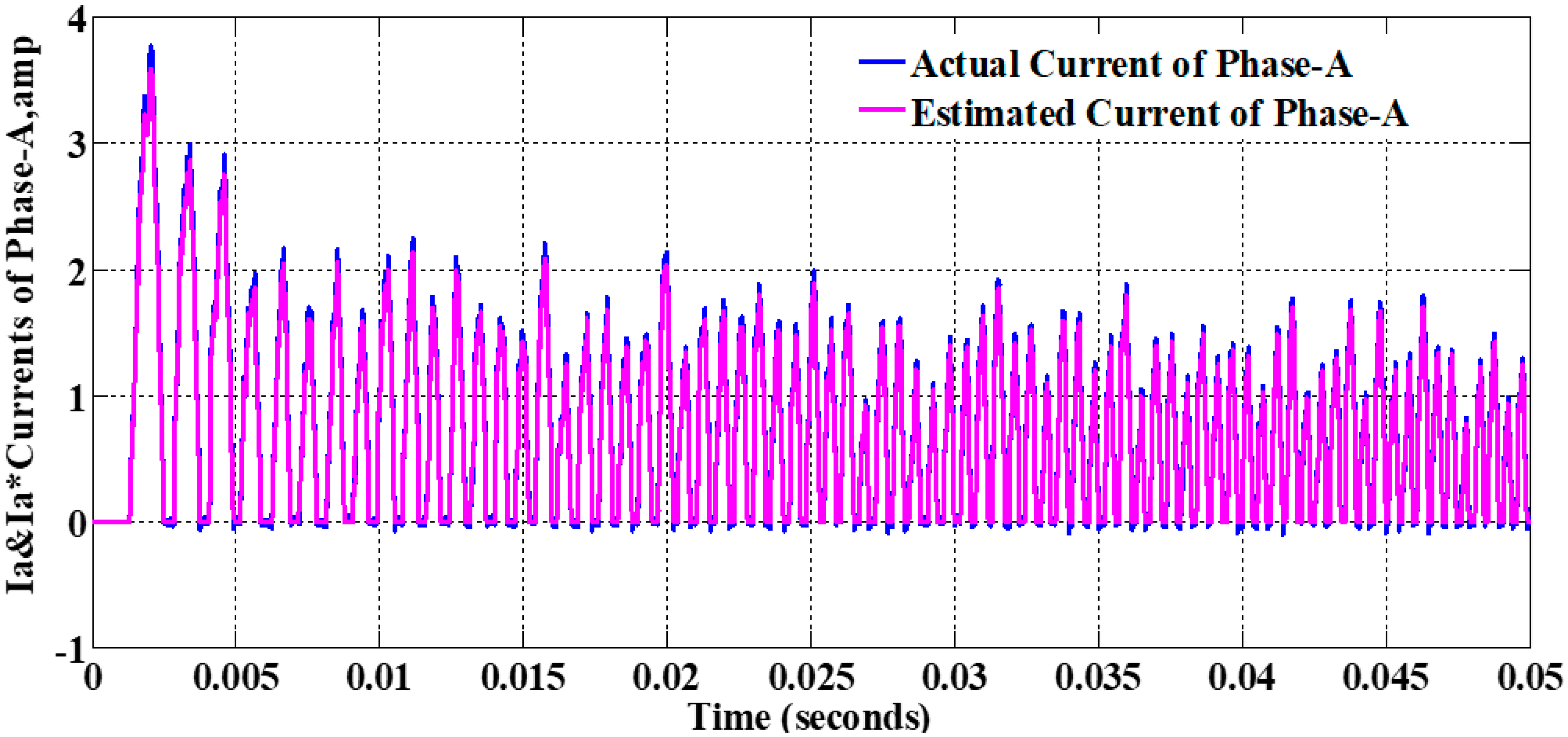
Figure 9.
Estimated and actual phase-A currents.
Figure 9.
Estimated and actual phase-A currents.
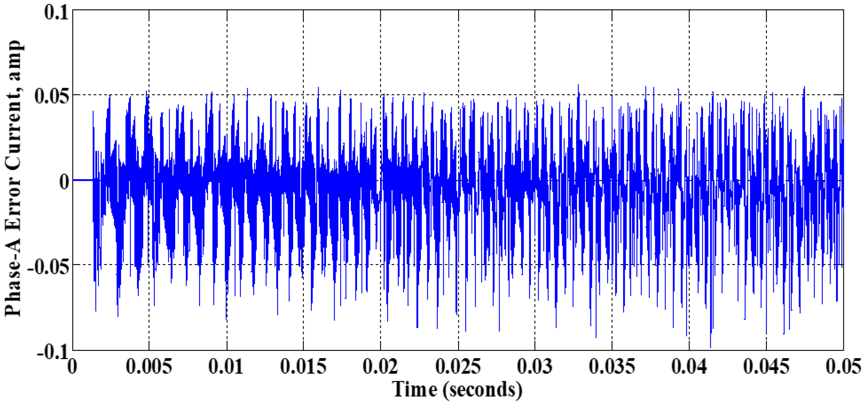
Figure 10.
Error between the estimated and actual currents of phase-A.
Figure 10.
Error between the estimated and actual currents of phase-A.
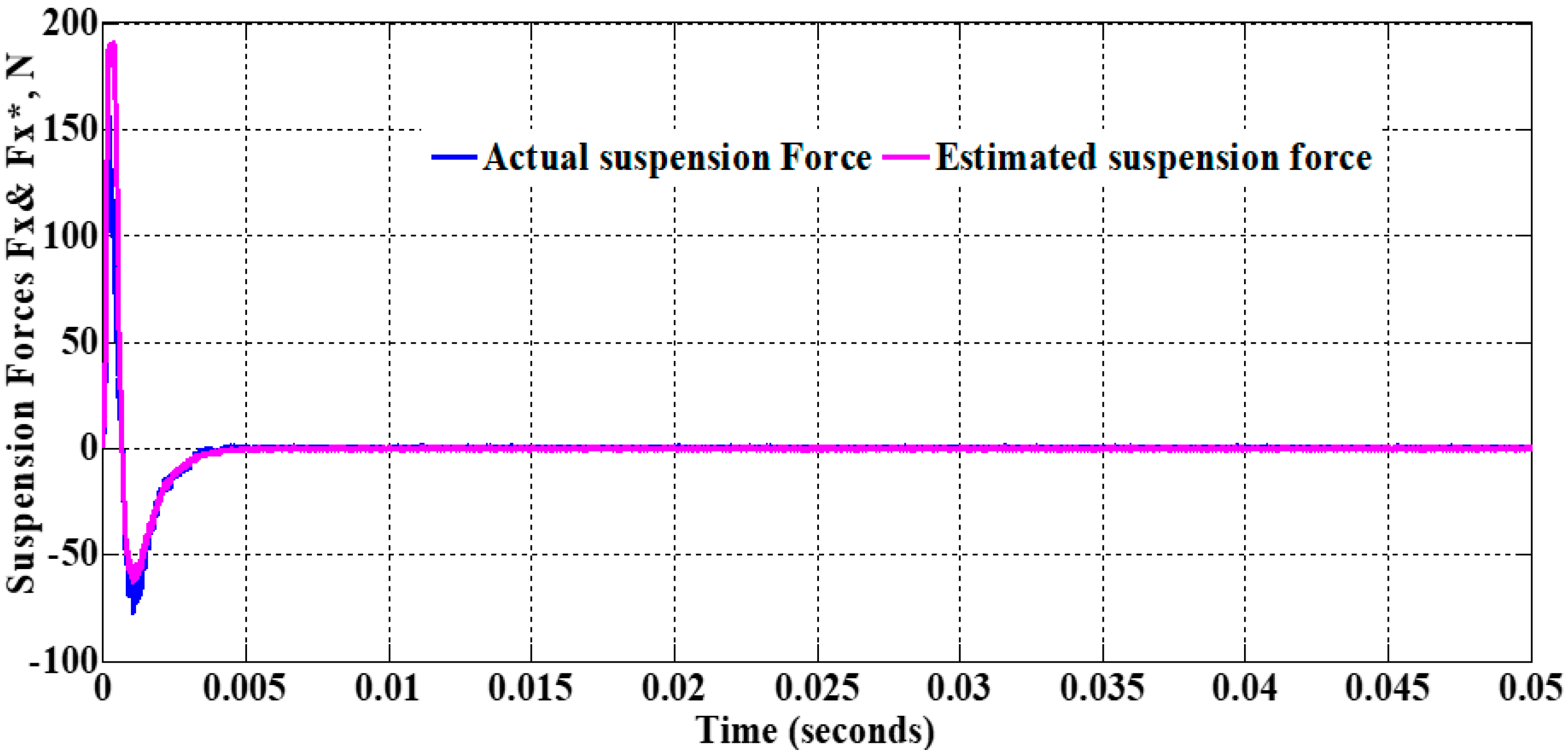
Figure 11.
Actual and estimated X-directional suspension forces.
Figure 11.
Actual and estimated X-directional suspension forces.
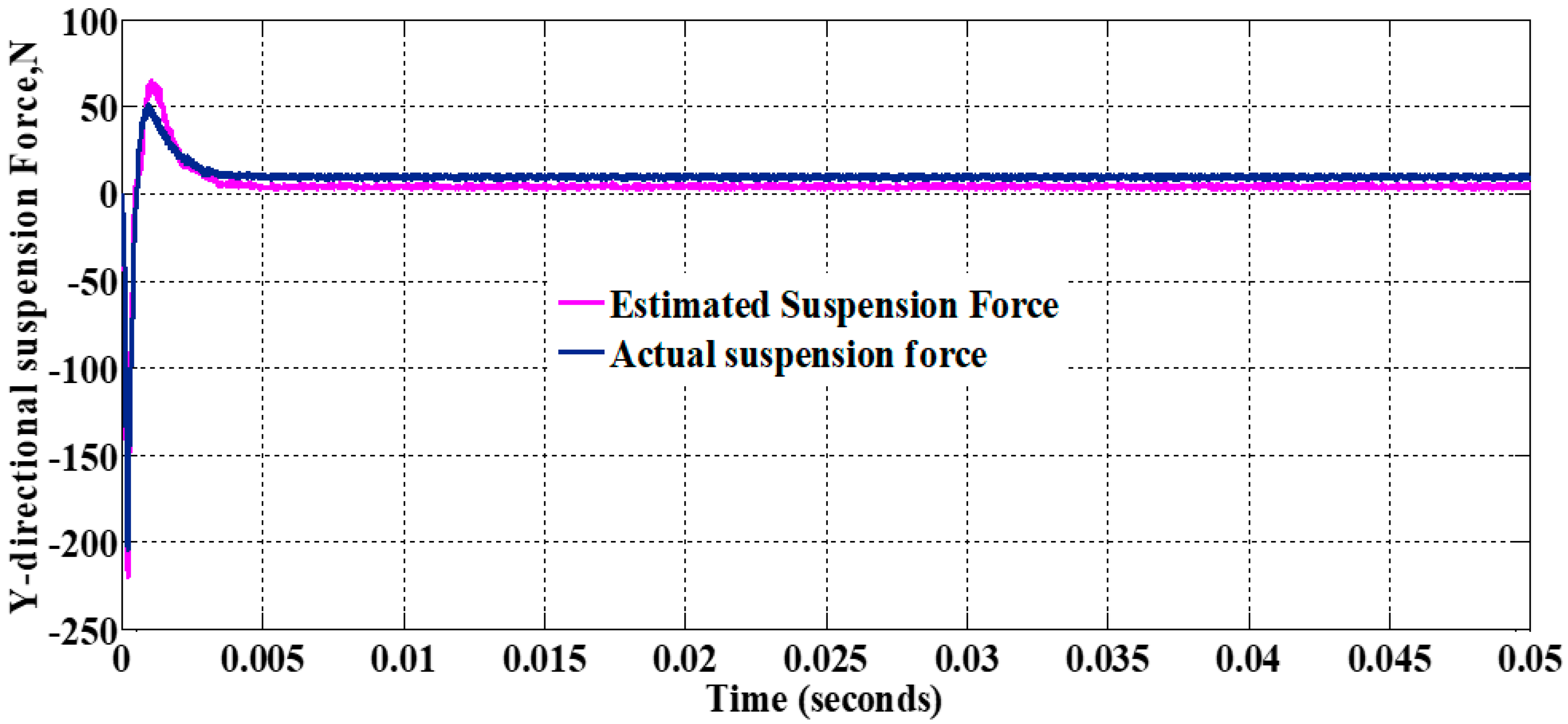
Figure 12.
Estimated and actual Y-directional suspension forces.
Figure 12.
Estimated and actual Y-directional suspension forces.
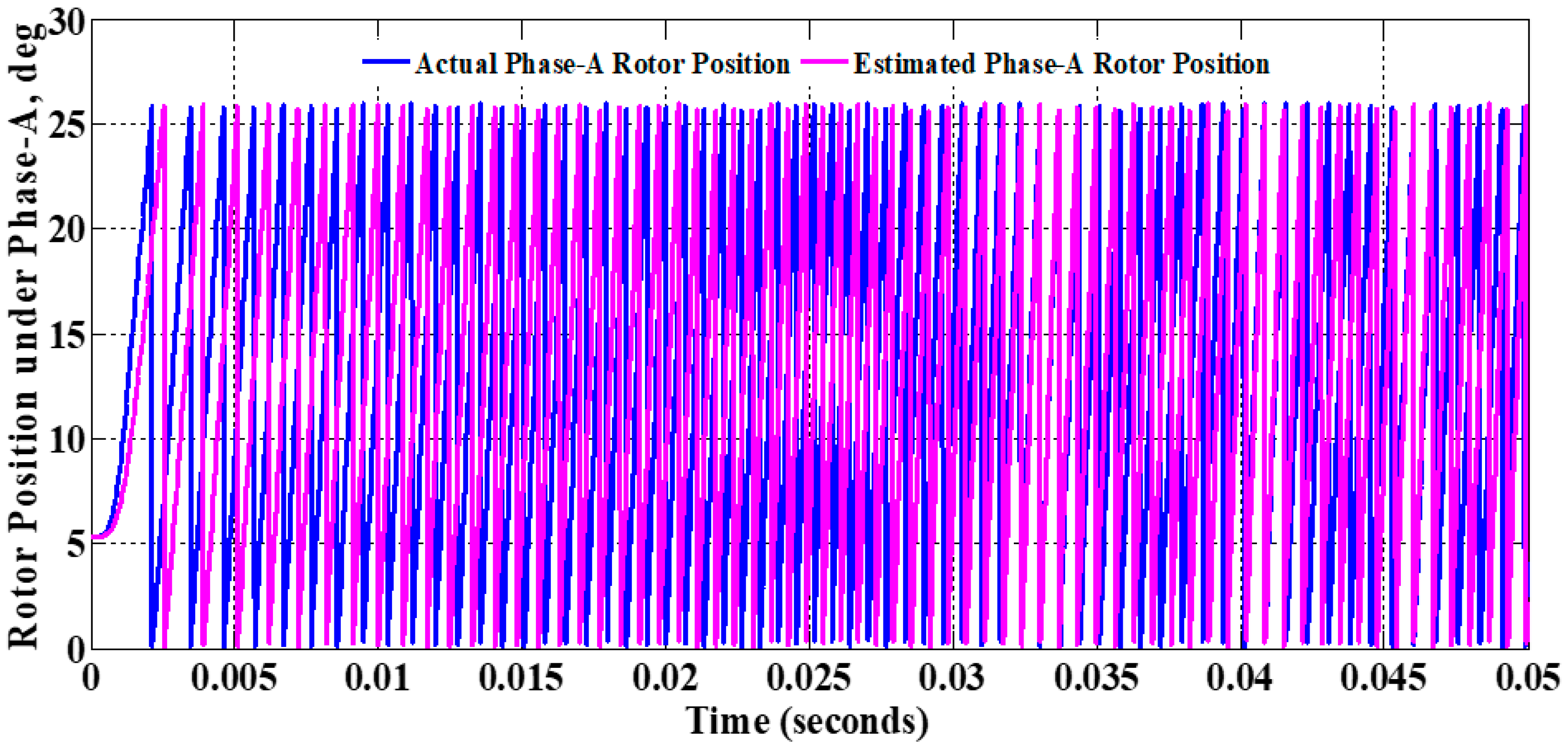
Figure 13.
Estimated and actual rotor positions under phase-A.
Figure 13.
Estimated and actual rotor positions under phase-A.
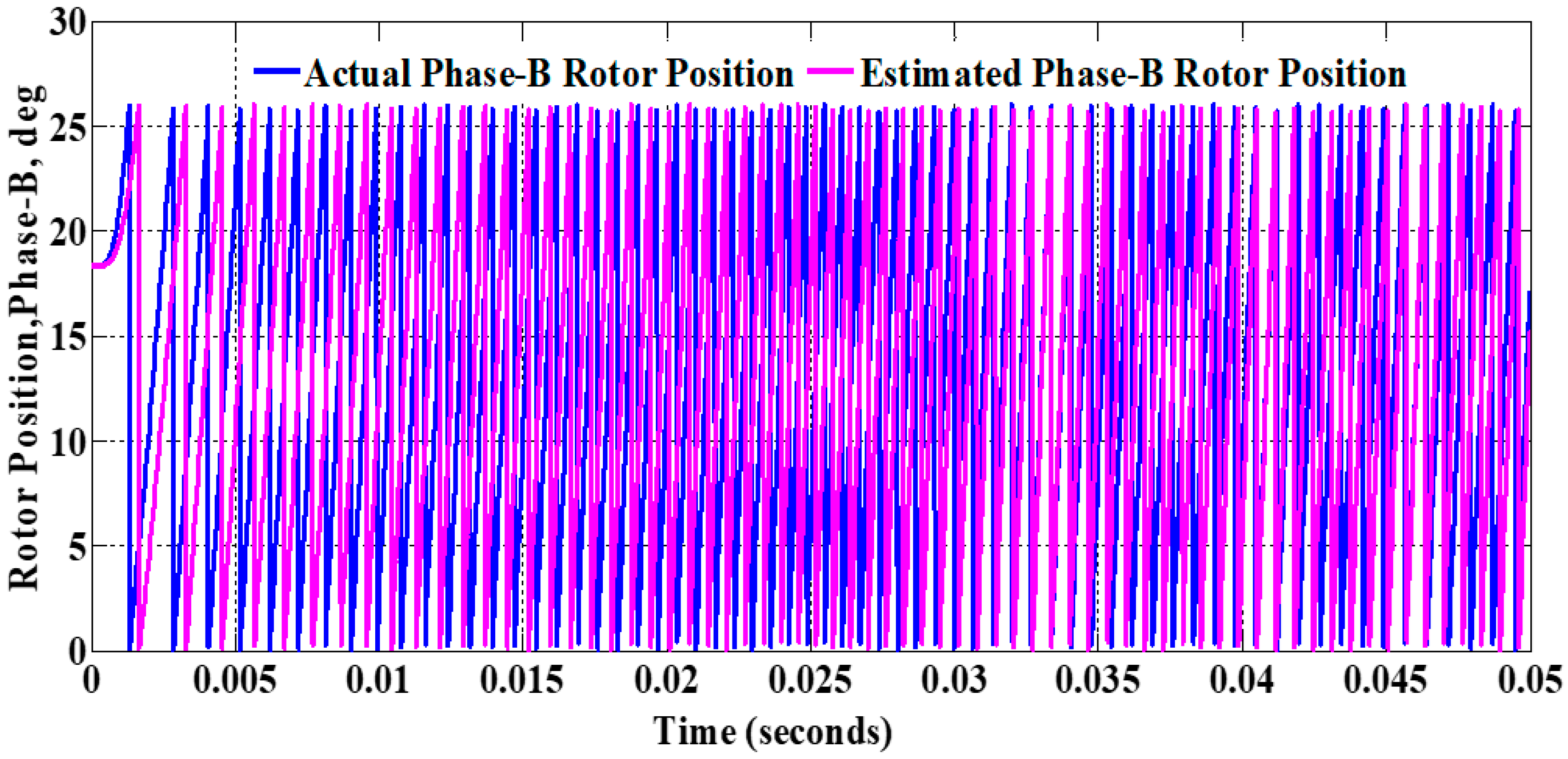
Figure 14.
Estimated and actual rotor positions under phase-B.
Figure 14.
Estimated and actual rotor positions under phase-B.
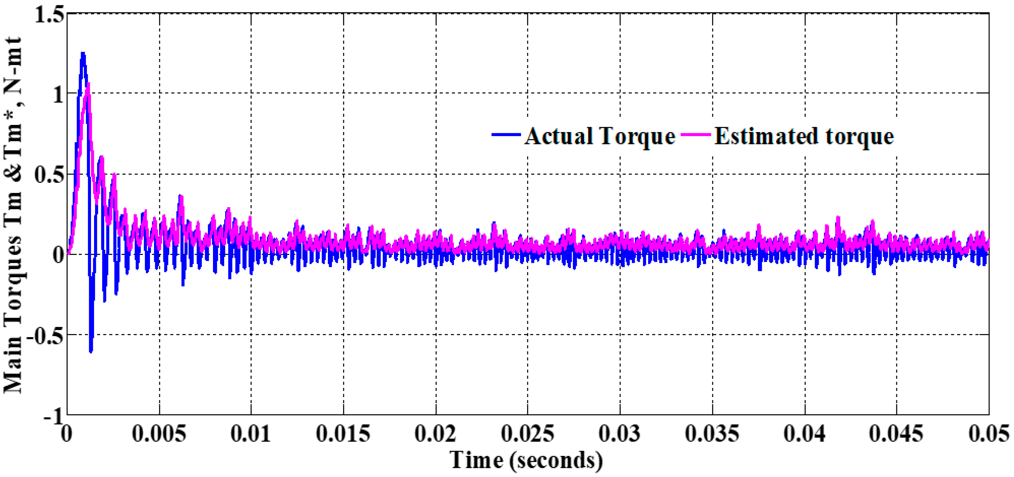
Figure 15.
Estimated and actual net torques.
Figure 15.
Estimated and actual net torques.
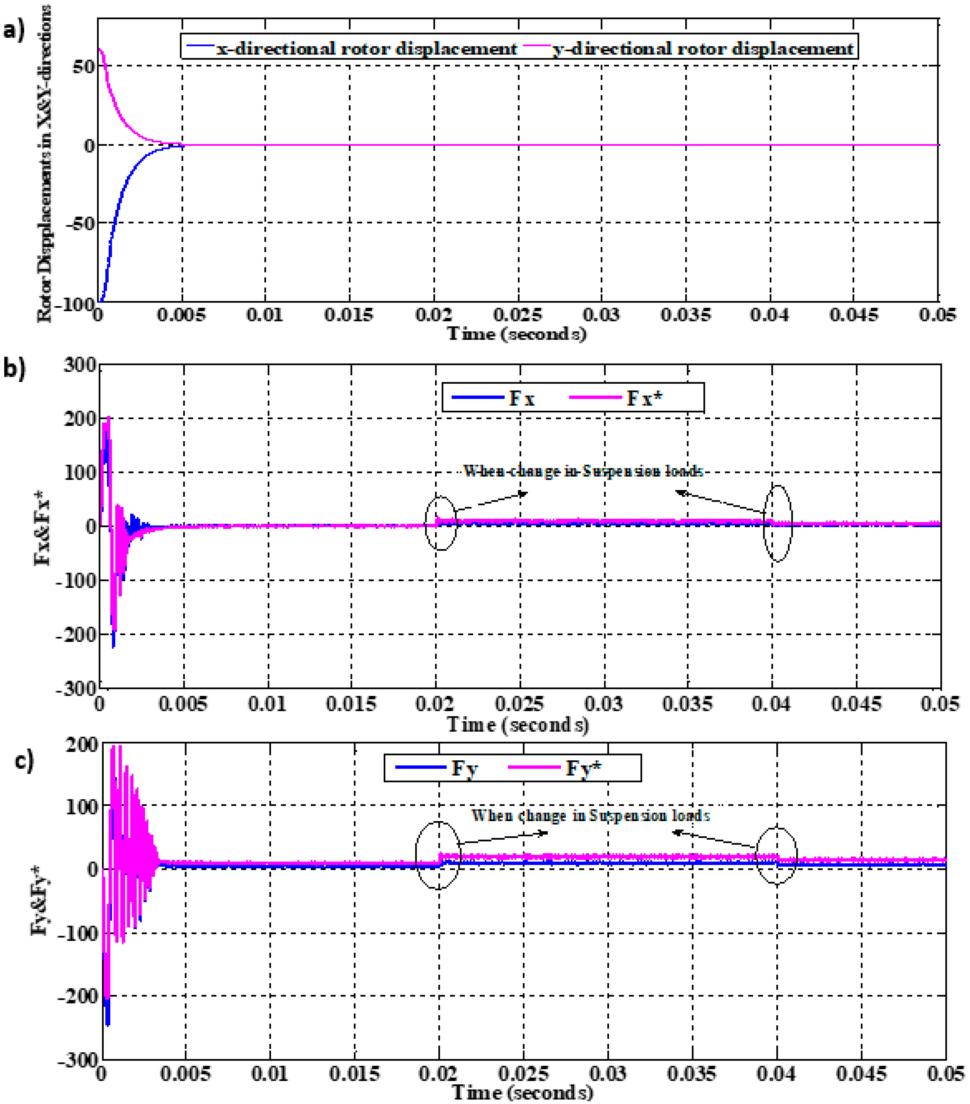
Figure 16.
(a) Rotor X and Y displacements, (b) actual and estimated X-directional suspension forces when suspension loads are applied, and (c) actual and estimated Y-directional suspension forces when suspension loads are applied.
Figure 16.
(a) Rotor X and Y displacements, (b) actual and estimated X-directional suspension forces when suspension loads are applied, and (c) actual and estimated Y-directional suspension forces when suspension loads are applied.
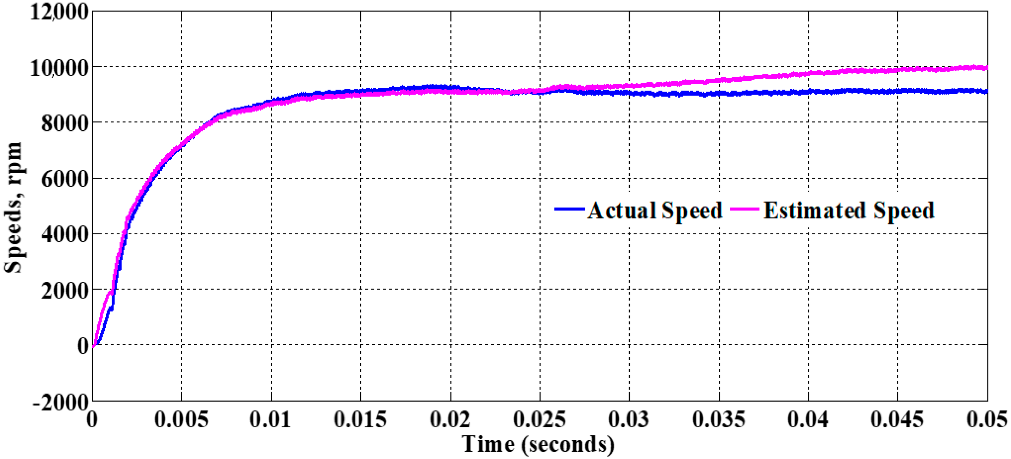
Figure 17.
Estimated and actual speeds.
Figure 17.
Estimated and actual speeds.
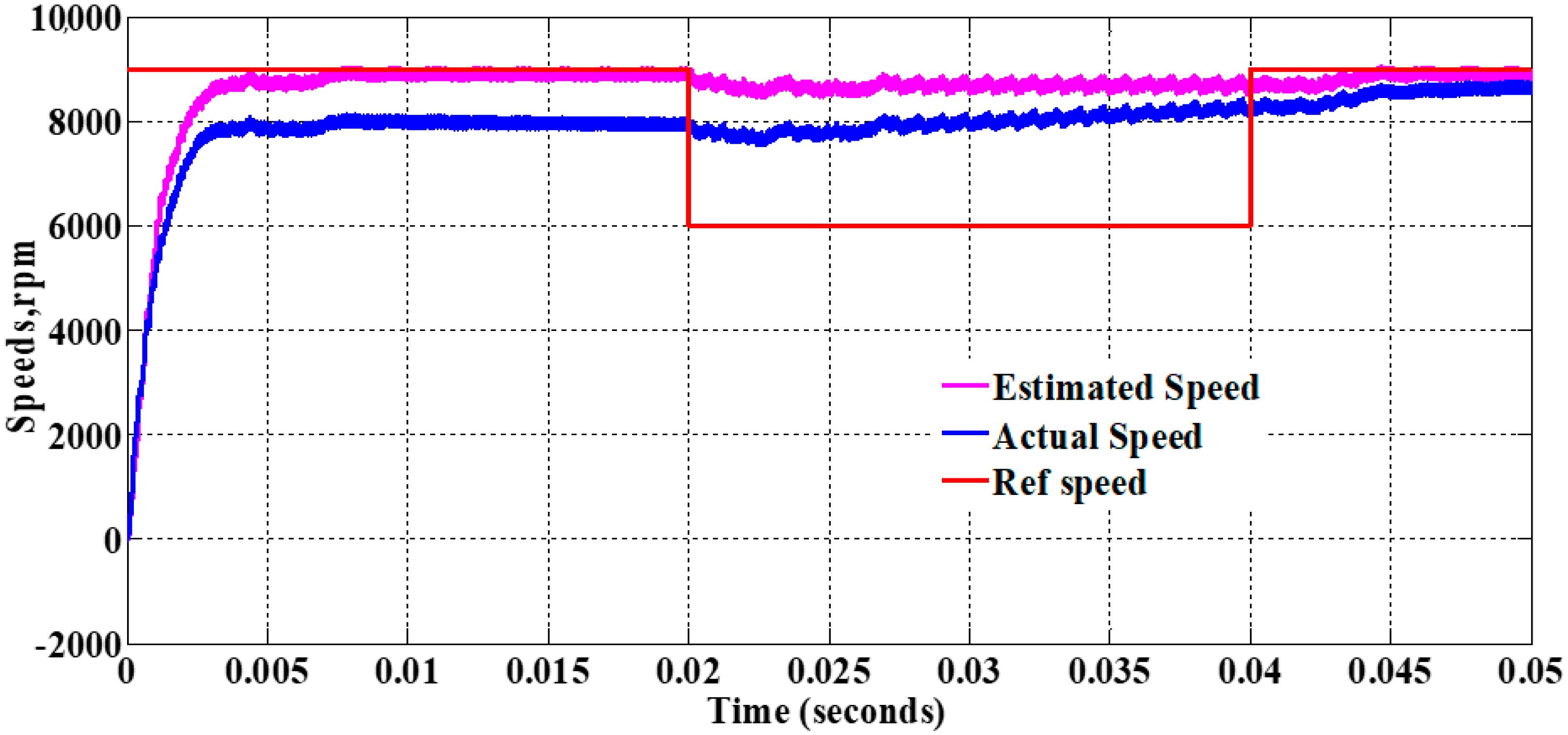
Figure 18.
Estimated and actual speeds.
Figure 18.
Estimated and actual speeds.
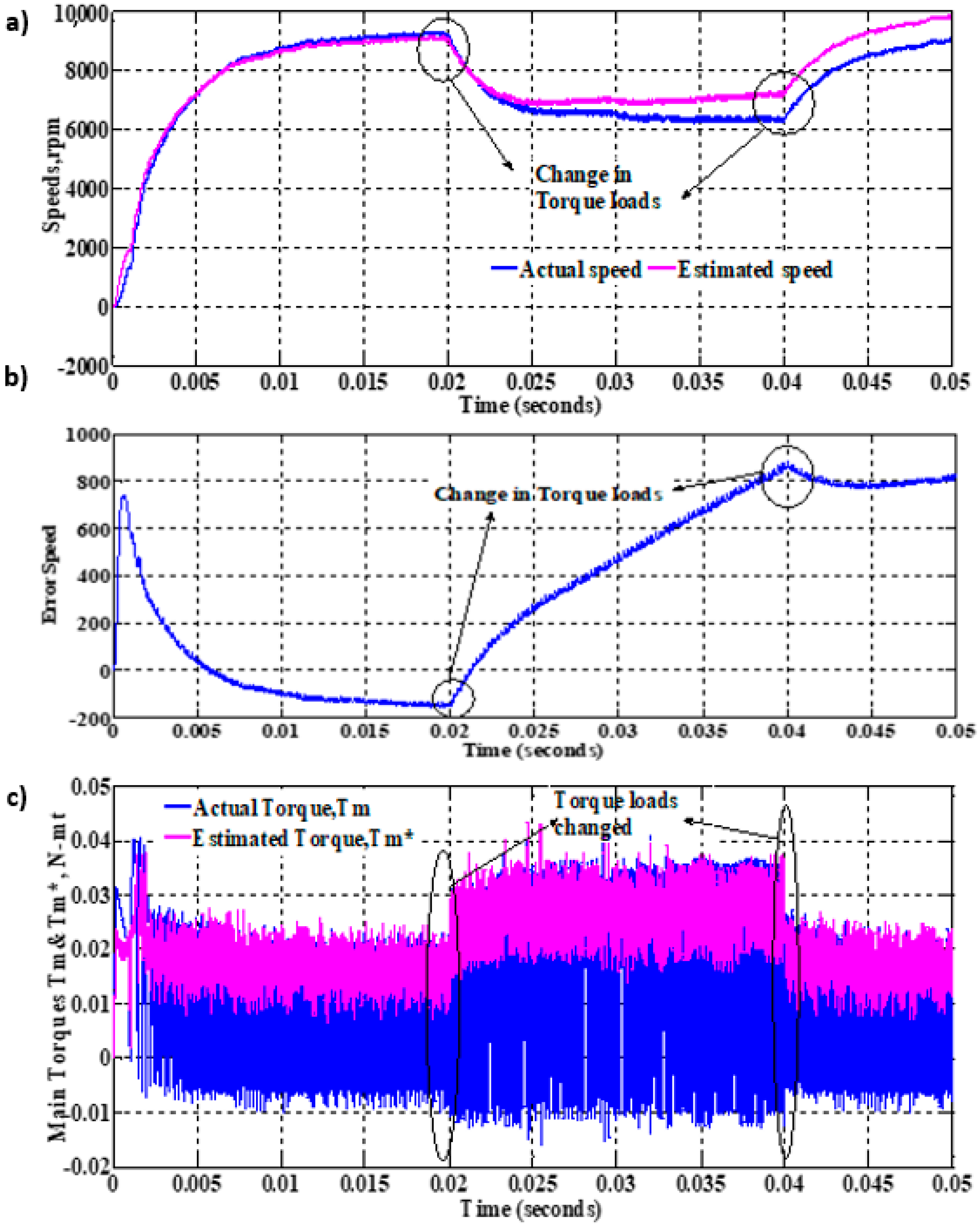
Figure 19.
(a) Estimated and actual speeds, (b) speed tracking error, and (c) estimated and actual net torque values when load torques varied.
Figure 19.
(a) Estimated and actual speeds, (b) speed tracking error, and (c) estimated and actual net torque values when load torques varied.
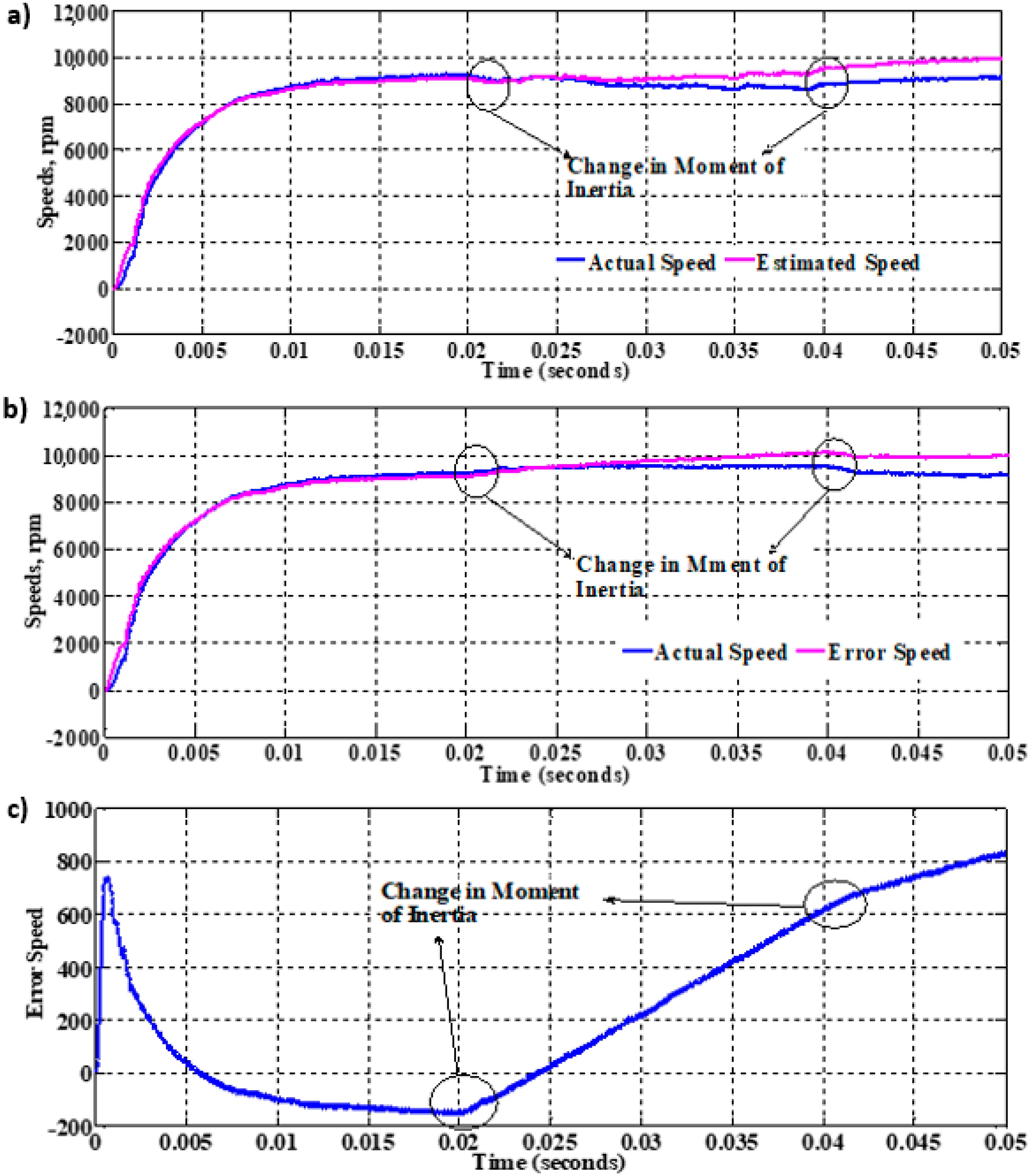
Figure 20.
(a) Estimated and actual speeds when there are increments in the moment of inertia, (b) Estimated and actual speeds when there are decrements of the moment of inertia, and (c) Speed tracking error for change of the moment of inertia.
Figure 20.
(a) Estimated and actual speeds when there are increments in the moment of inertia, (b) Estimated and actual speeds when there are decrements of the moment of inertia, and (c) Speed tracking error for change of the moment of inertia.
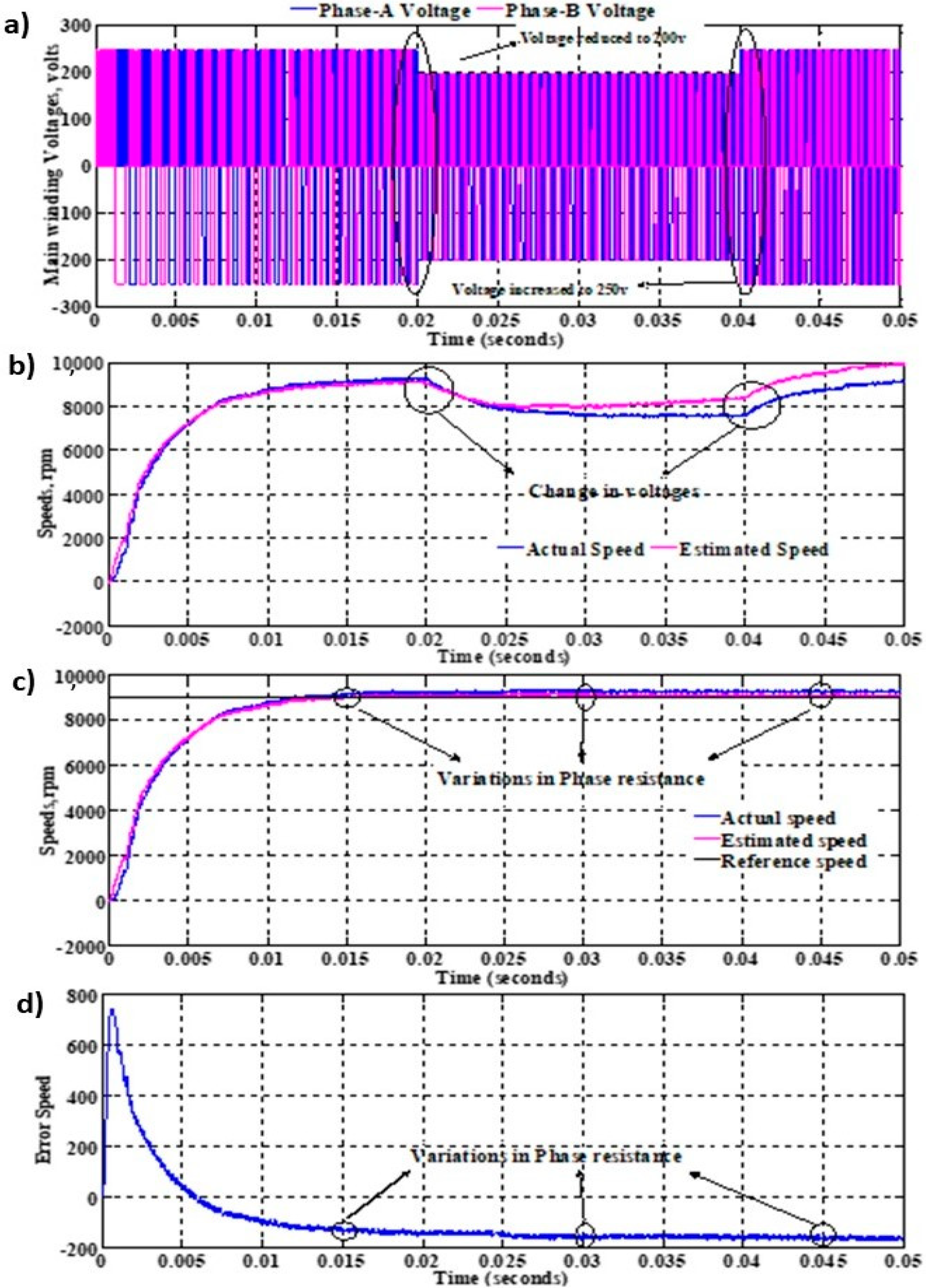
Figure 21.
(a) Regulated main phase voltages, (b) estimated and actual speeds when changes in the supply voltage, (c) Estimated and actual speeds when changes in phase resistances, and (d) speed tracking error when the phase resistances are varied.
Figure 21.
(a) Regulated main phase voltages, (b) estimated and actual speeds when changes in the supply voltage, (c) Estimated and actual speeds when changes in phase resistances, and (d) speed tracking error when the phase resistances are varied.
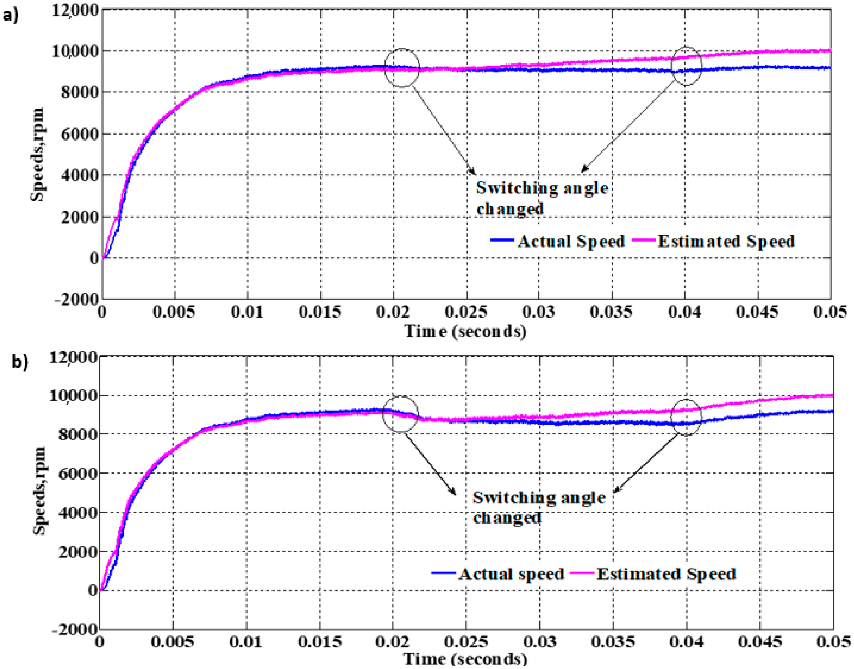
Figure 22.
(a) Estimated and actual speeds when switching angle is changed to 11 degrees and (b) Estimated and actual speeds when switching angle is changed to 13 degrees.
Figure 22.
(a) Estimated and actual speeds when switching angle is changed to 11 degrees and (b) Estimated and actual speeds when switching angle is changed to 13 degrees.
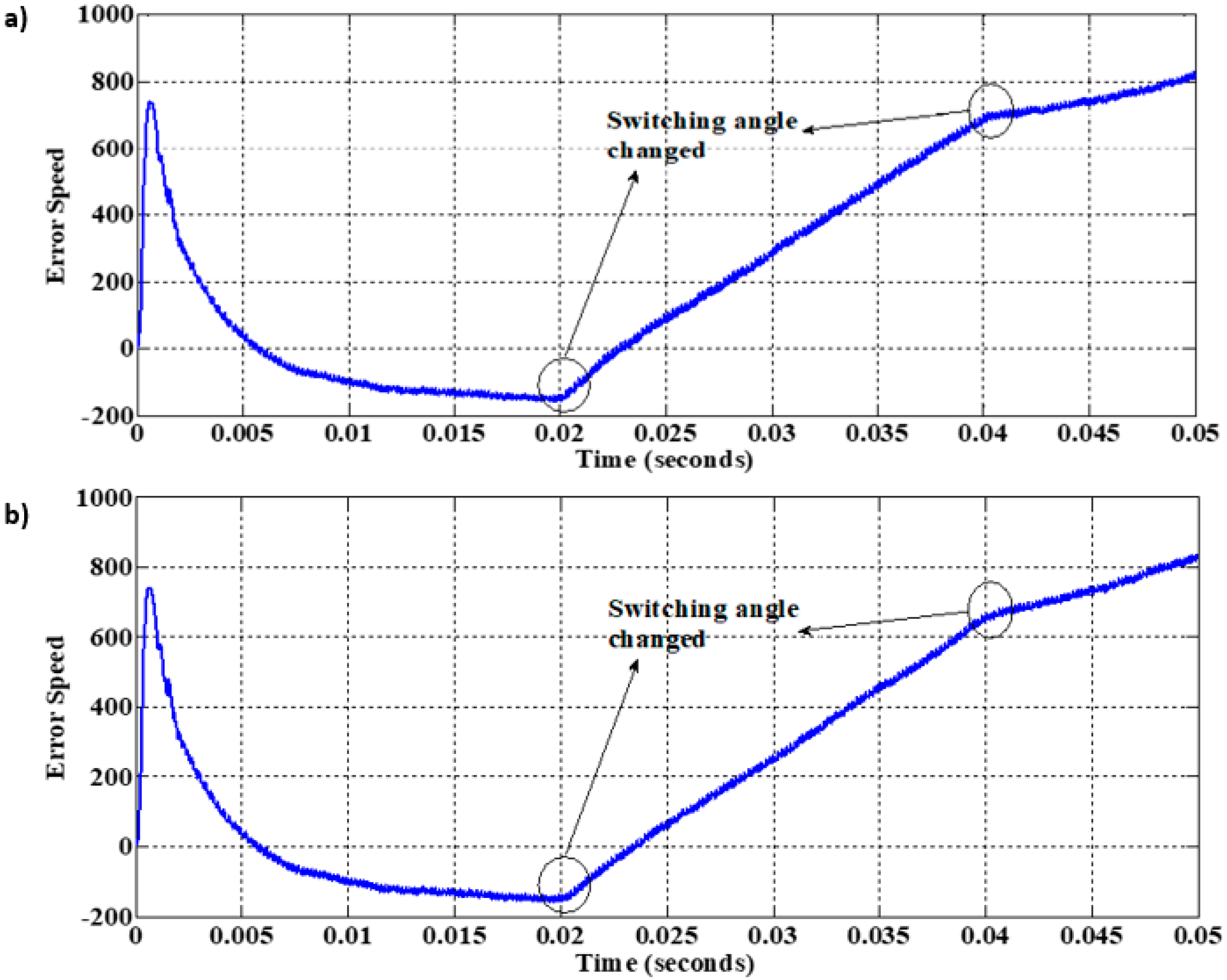
Figure 23.
(a) Speed-tracking error when switching angle is changed to 11 degrees (b) Speed-tracking error when switching angle is changed to 13 degrees.
Figure 23.
(a) Speed-tracking error when switching angle is changed to 11 degrees (b) Speed-tracking error when switching angle is changed to 13 degrees.
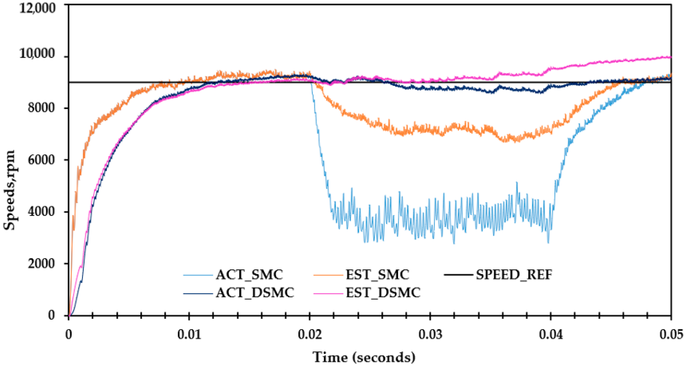
Figure 24.
Changes in the supply voltage. [Note: ACT_SMC: actual speed under sliding mode controller; EST_SMC: estimated speed under sliding mode controller; ACT_DSMC: actual speed under dynamic sliding mode controller; EST_DSMC: estimated speed under dynamic sliding mode controller; SPEED_REF: reference speed].
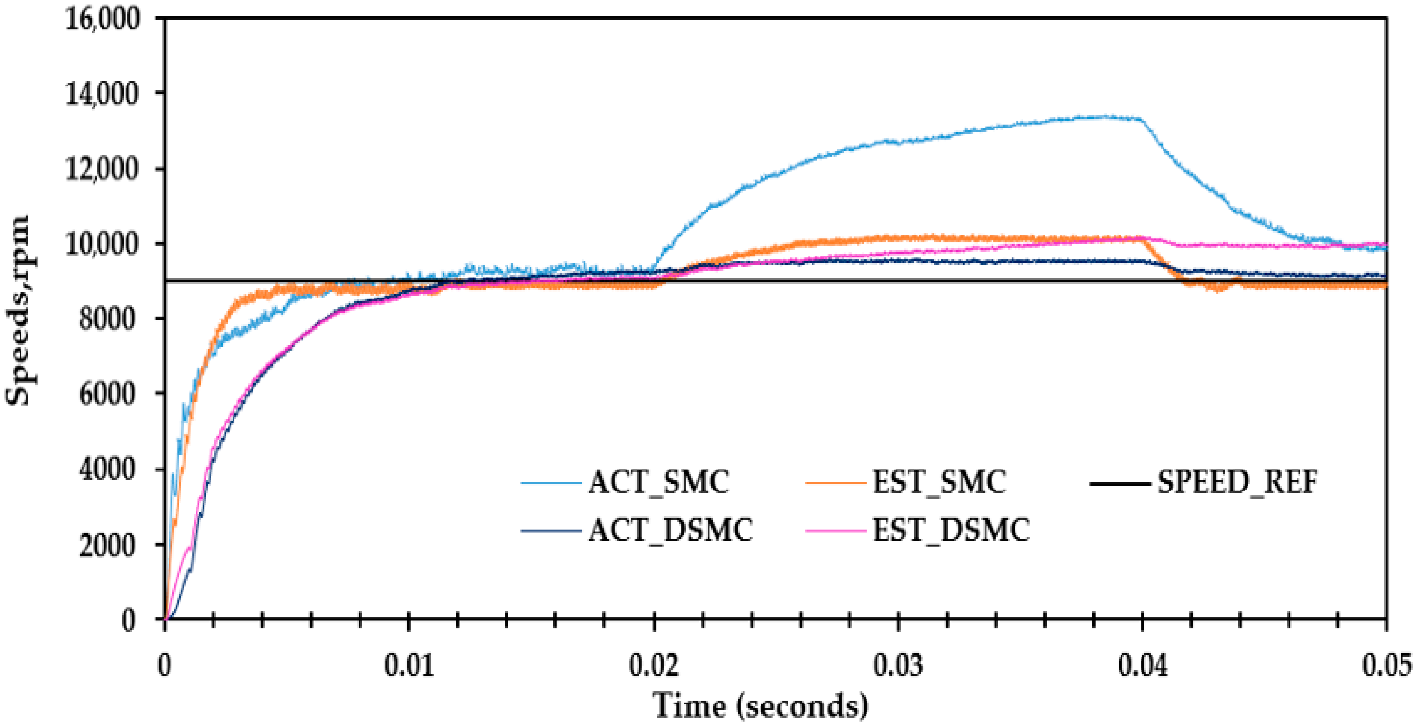
Figure 25.
Changes in the load torque. [Note: ACT_SMC: actual speed under sliding mode controller; EST_SMC: estimated speed under sliding mode controller; ACT_DSMC: actual speed under dynamic sliding mode controller; EST_DSMC: estimated speed under dynamic sliding mode controller; SPEED_REF: reference speed].
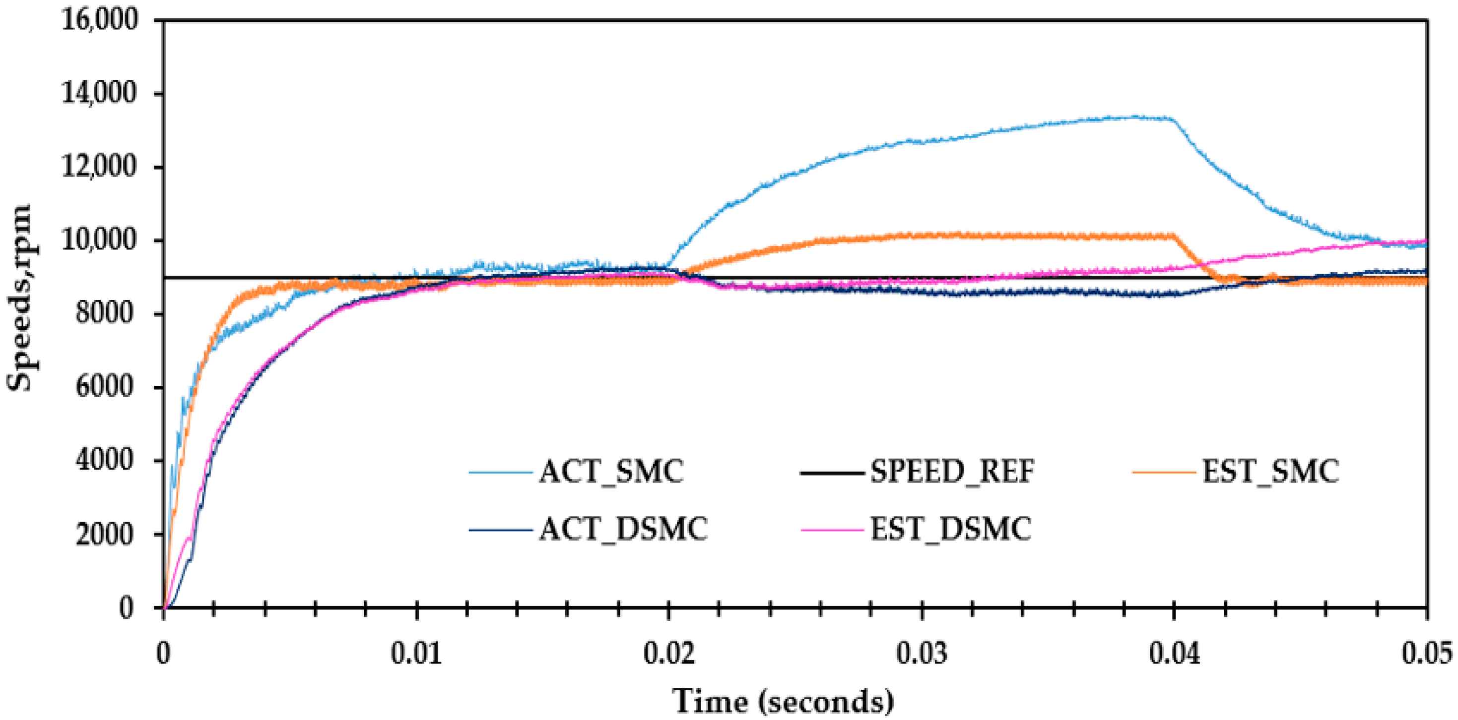
Figure 26.
Increments of the moment of inertia by 10%. [Note: ACT_SMC: actual speed under sliding mode controller; EST_SMC: estimated speed under sliding mode controller; ACT_DSMC: actual speed under dynamic sliding mode controller; EST_DSMC: estimated speed under dynamic sliding mode controller; SPEED_REF: reference speed].
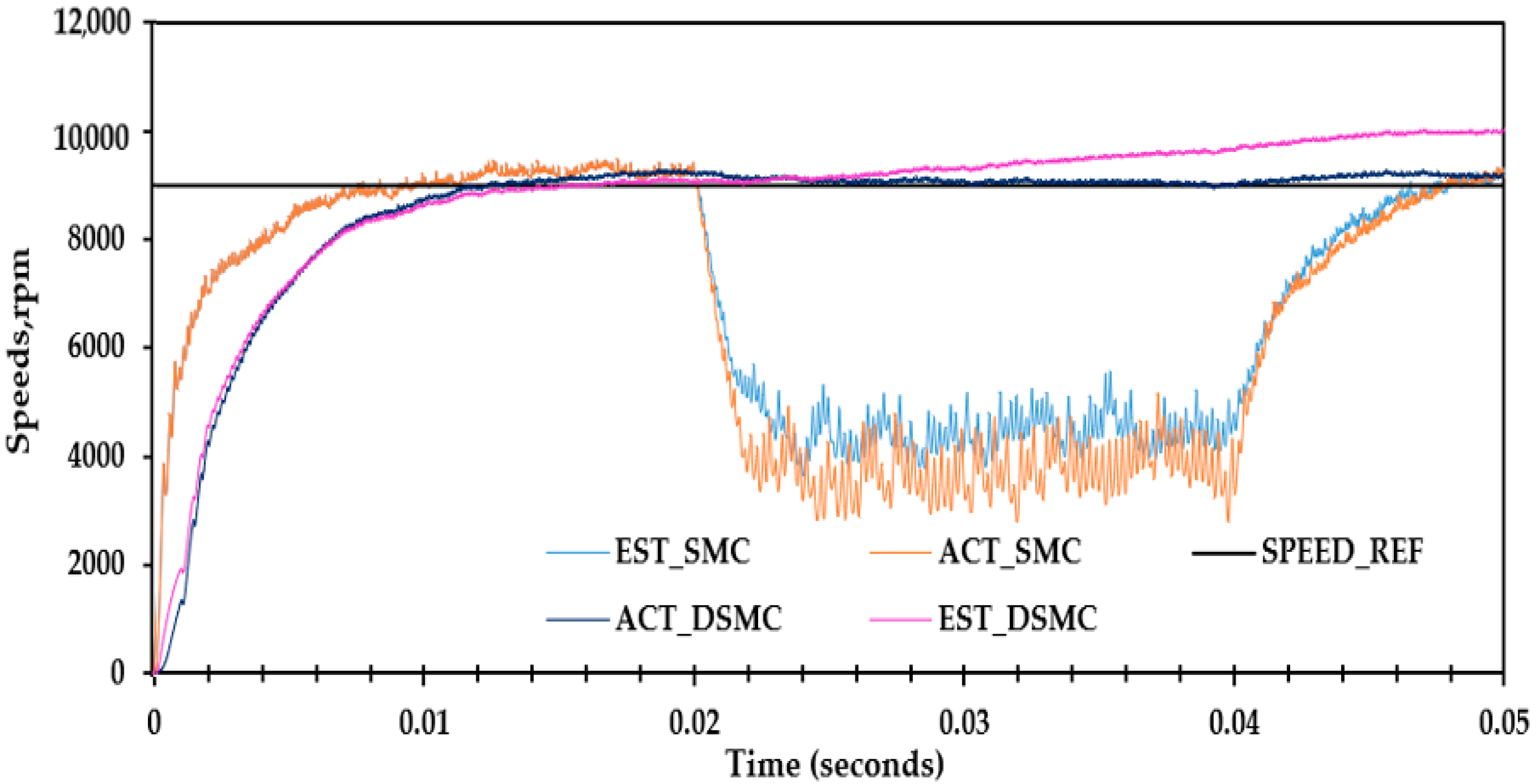
Figure 27.
Decrements of the moment of inertia by 10%. [Note: ACT_SMC: actual speed under sliding mode controller; EST_SMC: estimated speed under sliding mode controller; ACT_DSMC: actual speed under dynamic sliding mode controller; EST_DSMC: estimated speed under dynamic sliding mode controller; SPEED_REF: reference speed].
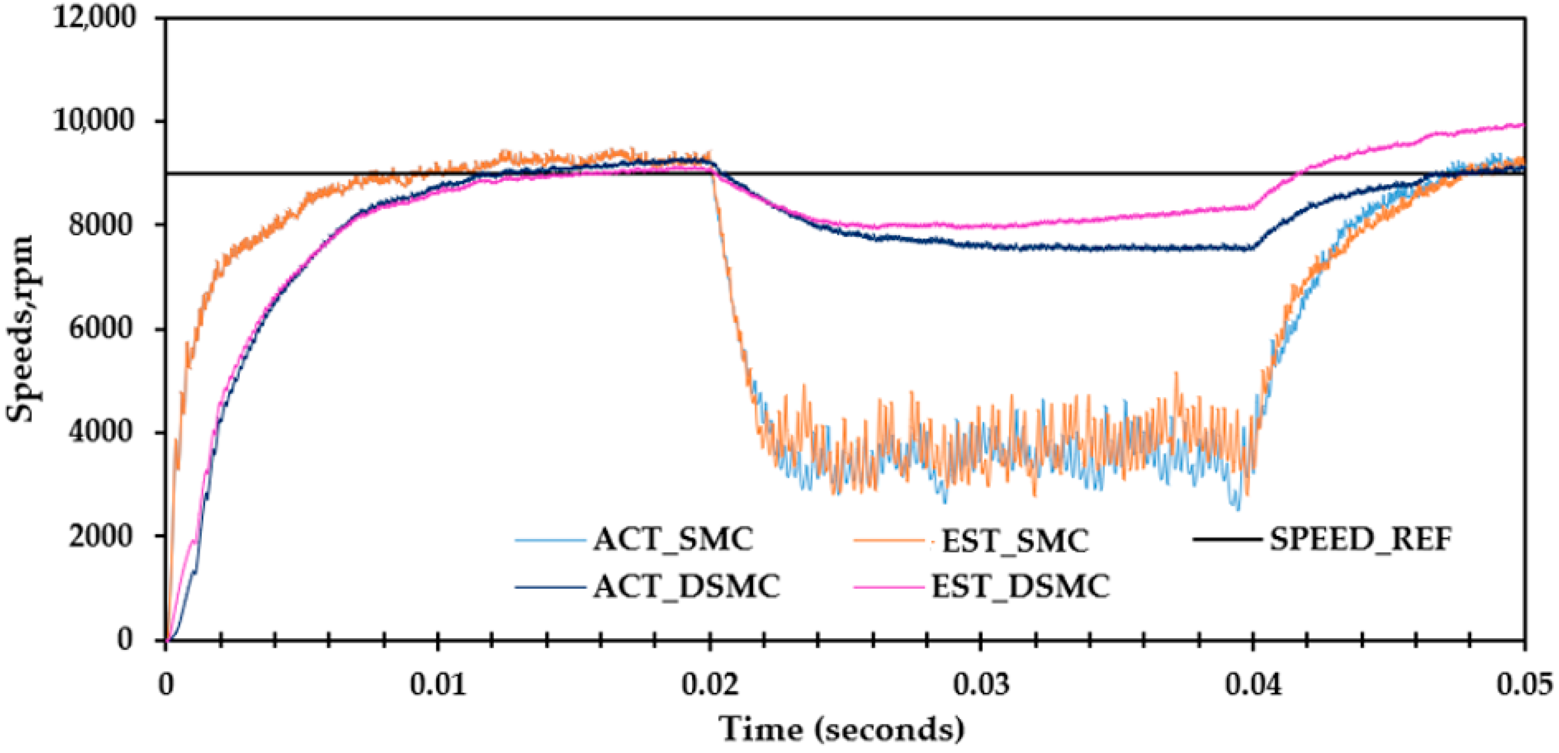
Figure 28.
Changes in the switching angle to 11 degrees. [Note: ACT_SMC: actual speed under sliding mode controller; EST_SMC: estimated speed under sliding mode controller; ACT_DSMC: actual speed under dynamic sliding mode controller; EST_DSMC: estimated speed under dynamic sliding mode controller; SPEED_REF: reference speed].
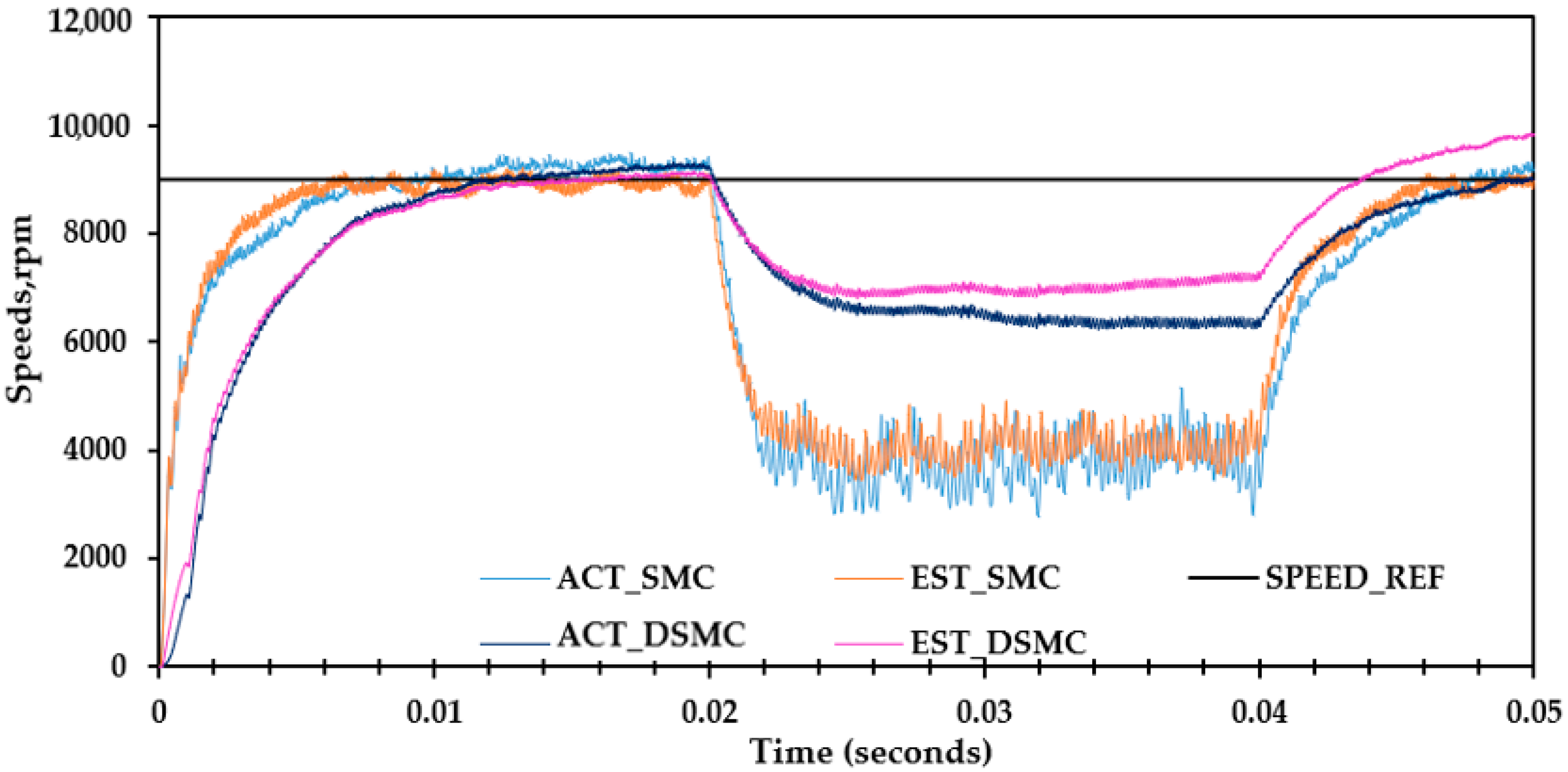
Figure 29.
Change in the switching angle to 13 degrees. [Note: ACT_SMC: actual speed under sliding mode controller; EST_SMC: estimated speed under sliding mode controller; ACT_DSMC: actual speed under dynamic sliding mode controller; EST_DSMC: estimated speed under dynamic sliding mode controller; SPEED_REF: reference speed].
Table 1.
Operating details of the 12/14 bearingless switched reluctance motor (BSRM).
Table 1.
Operating details of the 12/14 bearingless switched reluctance motor (BSRM).
| Parameters | Value |
|---|
| Rated power(motor) | 1 kW |
| Maximum motor Current/phase | 4 amp |
| Voltage/phase | 250 volts |
| Net torque | 1 Nm |
| Speed | 9000 rpm |
| Toque winding per phase resistance | 0.86 ohms |
| Suspension winding per phase resistance | 0.32 ohms |
| Suspension voltage | 250 volts |
| Maximum suspension current | 4 amp |
Table 2.
Switch numbers for the 12/14 bearingless switched reluctance motor (BSRM).
Table 2.
Switch numbers for the 12/14 bearingless switched reluctance motor (BSRM).
| 12/14 BSRM | Number of Power Switches | Total |
|---|
| Torque winding (two-phase) | 2 per phase | 4 |
| Suspending force winding (four-phase/four poles) | 2 per pole | 8 |
Table 3.
Switching state rule of the hysteresis control method for the bearingless switched reluctance motor (BSRM).
Table 3.
Switching state rule of the hysteresis control method for the bearingless switched reluctance motor (BSRM).
| Desired Force | Suspending Force Poles Selection | Enable Is1 | Enable Is2 | Enable Is3 | Enable Is4 |
|---|
| Is1 and Is2 | 1 | 1 | 0 | 0 |
| Is2 and Is3 | 0 | 1 | 1 | 0 |
| Is3 and Is4 | 0 | 0 | 1 | 1 |
| Is4 and Is1 | 1 | 0 | 0 | 1 |
Table 4.
Comparisons of speeds between the proposed and conventional methods.
Table 4.
Comparisons of speeds between the proposed and conventional methods.
| Parameters | SMC Based-SMO | DSMC-Based SMO |
|---|
| Change of system parameters | Difference in speed | % of Chattering | Difference in speed | % of Chattering |
| Change of Switching angle to 13 degree | 3000 | | 1000 | |
| Varying of supply voltage | 3500 | | 1500 | |
| Varying in load Torque | 3500 | | 1500 | |
| Decrease of moment of inertia by 10% | 3000 | | 800 | |
| Increase of moment of inertia by 10% | 2000 | | 800 | |
| Change of Switching angle to 11 degree | 2000 | | 1000 | |


 ,
, 


