Article

Development of Advanced Computer Aid Model for Shear Strength of Concrete Slender Beam Prediction

by
Ahmad Sharafati
1,2,3,
Masoud Haghbin
3,
Mohammed Suleman Aldlemy
4,
Mohamed H. Mussa
5,6,
Ahmed W. Al Zand
5,
Mumtaz Ali
7,
Suraj Kumar Bhagat
8,
Nadhir Al-Ansari
9 and
Zaher Mundher Yaseen
10,*
1
Institute of Research and Development, Duy Tan University, Da Nang 550000, Vietnam
2
Faculty of Civil Engineering, Duy Tan University, Da Nang 550000, Vietnam
3
Department of Civil Engineering, Science and Research Branch, Islamic Azad University, Tehran, Iran
4
Department of Mechanical Engineering, Collage of Mechanical Engineering Technology, Benghazi, Libya
5
Department of Civil Engineering, Faculty of Engineering & Built Environment, Universiti Kebangsaan Malaysia (UKM), Bangi 43600, Selangor, Malaysia
6
Department of Civil Engineering, University of Warith Al-Anbiyaa, Karbala 56001, Iraq
7
Deakin-SWU Joint Research Centre on Big Data, School of Information Technology, Deakin University, Victoria 3125, Australia
8
Faculty of Civil Engineering, Ton Duc Thang University, Ho Chi Minh City, Vietnam
9
Civil, Environmental and Natural Resources Engineering, Lulea University of Technology, 97187 Lulea, Sweden
10
Sustainable Developments in Civil Engineering Research Group, Faculty of Civil Engineering, Ton Duc Thang University, Ho Chi Minh City, Vietnam
*
Author to whom correspondence should be addressed.
Appl. Sci. 2020, 10(11), 3811; https://doi.org/10.3390/app10113811
Submission received: 31 March 2020 / Revised: 14 May 2020 / Accepted: 27 May 2020 / Published: 30 May 2020
(This article belongs to the Special Issue Health Structure Monitoring for Concrete Materials, Volume II)

Abstract

:
High-strength concrete (HSC) is highly applicable to the construction of heavy structures. However, shear strength (Ss) determination of HSC is a crucial concern for structure designers and decision makers. The current research proposes the novel models based on the combination of adaptive neuro-fuzzy inference system (ANFIS) with several meta-heuristic optimization algorithms, including ant colony optimizer (ACO), differential evolution (DE), genetic algorithm (GA), and particle swarm optimization (PSO), to predict the Ss of HSC slender beam. The proposed models were constructed using several input combinations incorporating several related dimensional parameters such as effective depth of beam (d), shear span (a), maximum size of aggregate (ag), compressive strength of concrete (fc), and percentage of tension reinforcement (ρ). To assess the impact of the non-homogeneity of the dataset on the prediction result accuracy, two possible modeling scenarios, (i) non-processed (initial) dataset (NP) and (ii) pre-processed dataset (PP), are inspected by several performance indices. The modeling results demonstrated that ANFIS-PSO hybrid model attained the best prediction accuracy over the other models and for the pre-processed input parameters. Several uncertainty analyses were examined (i.e., model, variables, and data), and results indicated predicting the HSC shear strength was more sensitive to the model structure uncertainty than the input parameters.

1. Introduction

Among the high-performance concrete (HPC) used in structural engineering, high-strength concrete (HSC) has received the most significant attention. The HSC is used in several structural engineering projects and is mostly considered at a compressive strength of >60 MPa due to the benefits it offers [1]. Despite the lack of a clear difference between HSC and normal-strength concrete (NSC), several approaches and studies have determined varying ranges of compressive strength (CS) for differentiating NSC from HSC [2]. This study, however, followed the ACI 363R-10, which described HSC as concrete with CS of >40 MPa [3]. HSC has significant benefits, which have boosted its implementation in construction activity globally. Such advantages include its improved physicomechanical properties such as CS, long-term durability, and stiffness. HSC attracts great interest due to the economic usefulness associated with it as it helps in reducing geometrical sections and gain in structures. Thus, HSC is preferred over NSC for economic, aesthetic, and technical purposes [4]. Practically, HSC is known to be brittle [4] as studies have shown sudden cracking and traversing aggregate particles in HSC, which produces fracture planes that are relatively smooth [5]. As with NSC, these cracks do not cover whole aggregate particles. Concrete shear strength is significantly reduced by smooth fracture surfaces by reducing the aggregate interlock contribution at the shear fracture planes.
For a reinforced concrete (RC) beam without transverse reinforcement, its failure mechanism can be considered as the generation of three internal forces that contribute to shear resistance. These internal forces include the concretes’ contribution in the compression region (Vc), the shear contribution due to the dowel action of longitudinal rebars (Vd), and the shear contribution due to the aggregate interlock (Va). Consequently, the overall shear resistance is the summation of all these internal forces. Components Va and Vd are ineffective if the diagonal crack opening is excessive. As a result, all the shear on the section will be on component Vc, leading to beam collapse as the concrete is crushed in compression [6].
The shear capacity of beams is mainly influenced by the aggregate interlocking mechanism; thus, the beams’ ultimate load capacity under shear is influenced by this mechanism [7,8]. As per [9], Va for beams of CS ranging between 26 and 49 MPa accounts for 33% to 50% of the overall shear resistance of such beams. However, Va seems not to contribute significantly towards shear at higher concrete strengths as evidenced by the smooth fracture planes and straight cracks, which do not cover the whole aggregates as earlier mentioned. Similarly, [10] suggested taking Va as zero for concrete with CS of >62 MPa.
Based on the existing literature on RC shear slender beams without web reinforcement, it is evident that no common rational theory exists to explain the collaboration between the three internal forces that contribute to shear resistance, particularly for HSC [11]. It appears that the precise estimation of shear capacity of HCS slender RC beam in the absence of shear stirrups is an open topic in research communities of structural engineering [12,13]. The relationship between the intricate modeling variable has a remarkable influence on the shear capacity of HSC slender beams without stirrups. As such, the regression-based models are not considered ideal for such an application [14]. The existing stochasticity or nonlinearity in the experimental database initiates a very complex regression problem that needs a sophisticated modeling approach to mimic its actual internal mechanism. Artificial intelligence (AI) models have found wide application in solving different problems in civil engineering due to their interesting features, such as their auto-search and adaptation capability when finding multi-variable interrelationships [15,16,17,18,19,20]. The shear strength (Ss) problem related to the structural engineering field has been investigated using the feasibility of AI models that have demonstrated positive progress [8,21,22].
Several versions of AI models have been developed for beam Ss prediction, such as artificial neural network (ANN) [15,23,24,25], support vector machine (SVM) [26,27,28,29], evolutionary computing models (ECM) [30,31,32,33], and adaptive neuro-fuzzy inference system (ANFIS) [34,35,36,37,38]. Among all the aforementioned AI models, ANFIS confirmed its potential in modeling beam Ss mechanisms over the other models. The ANFIS model is characterized by the capability to mimic and capture the associated non-linearity and stochasticity of data time series [39]. However, the ANFIS model is associated with a major drawback, which is the membership function tuning parameters. Thus, combining the optimization algorithms, which are inspired by the behavior of animals and plants in nature, with a standalone ANFIS model appears as a new alternative model for improving its performances in solving difficult problems [40,41]. The hybrid ANFIS model exhibited a noticeable implementation for diverse civil engineering applications [42,43,44]. In the current research, some parameters of the optimization algorithms (e.g., mutation probability) were assigned based on the reported literature review studies, while the appropriate values of those parameters can be obtained using the Taguchi approach [45]. This study assumes that the prediction modeling is associated with only input variables and model structures uncertainties, while the other uncertainty sources such as measurement errors, data handling, and inadequate sampling were ignored. The modeled dataset was hypothesized to be associated with redundant observations, and thus the dataset was constructed based on two scenarios of non-processed and pre-processed.
The main motivation of this study is to investigate the feasibility of the novel hybrid ANFIS models for modeling high-strength concrete beam Ss. The modeling procedure is involved in several experiments of HSC slender beams. Being that deep beams behave differently compared to the slender beams (owing to size effect), only slender beams were used in this research. The data analysis focused on ascertaining the model validity and establishing its limitations. Before the prediction process, several input combinations were constructed using the related physical properties including the effective depth of beam (d), shear span (a), maximum size of aggregate (ag), compressive strength of concrete (fc), and percentage of tension reinforcement (ρ). The Ss of the HSC slender beams is predicted using two different modeling scenarios based on (i) non-processed (initial) dataset (NP) and (ii) pre-processed dataset (PP) to investigate the impact of the non-homogeneity of the dataset on prediction result accuracy.

2. Materials and Methods

2.1. Database Description

An experimental dataset of HSC slender beams which fails in shear has been selected for constructing the applied hybrid AI models. The data were gathered from 33 intensive published types of research from between 1957 and 2013 [4,46,47,48,49,50,51,52,53,54,55,56,57,58,59,60,61,62,63,64,65,66,67,68,69,70,71,72,73,74,75,76,77]. Total observations of the dataset are 250, which are based on rectangular HSC slender RC beams. In general, the data were selected based on geometric and material characteristics appearance. Furthermore, the followings precise standards were considered strictly during the selection of the esteemed database:
i.
The selection of beams was based on those that were longitudinally reinforced with pre-stressed and fewer steel rebars and lack of shear stirrups.
ii.
Shear failure was the primary benchmark for the specimens which were uniformly loaded along with one or two weights.
iii.
Range of shear span (a) was observed between 399–2745, where the data are skewed right (Skewness = 1.85) and leptokurtic (Kurtosis = 3.73). However, in the case of ag/d, the calculated value was found to be between 0.010811–0.176056, where data were characterised by leptokurtic (kurtosis = 2.02) but considerably symmetric skewness (0.33).
iv.
The majority (83.6%) of observations contained the range of effective depth of beam (d) from 133 to 300 mm; besides, 65.2% of data lie between 200 and 300 mm.
v.
Acceptance of the dimension of the shear span was ≥ 2.5 times the a/d (effective depth), where the majority (84%) of the data falls in the 2.5–4 range of a/d. Moreover, ag varies from 9.5 to 25.4 mm, where 92.0% of the dataset contains the maximum size of aggregate between 9.5 and 19 mm.
vi.
Most of the data (92%) contain the aggregate size between 9.5 and 19 mm; in case of compressive strength of concrete ( f c ) , 90% of the data lie at ≤ 100 MPa of f c , and 4% out of 100 MPa. Among 90%, the majority (56%) were between 40–60 MPa; in case of the percentage of tension reinforcement ( ρ ), the majority of the data (91.2%) are up to 4%.
It is worth mentioning that there are some limitations in the data which have not been considered, such as rebar diameter, the concrete tensile strength, the initial shrinkage/thermal strains at early ages, which might have an impact on shear strength of HCS slender RC beams due to being absent in the database; hence, these have been excluded from this study.

2.2. Soft Computing Models Overview

Artificial intelligence models are used to solve complex engineering applications associated with non-linear phenomena that cannot be generally solved using classical regression models. AI models eliminate the disadvantages of hard computing simulation. For instance, hard computing requires exact models, but since the AI model’s procedure is similar to a black box, the problem does not need to be perfectly modeled. Hence, AI can consider both partial truth and approximation, and models that are soft computing methods can incorporate uncertainty. The goal of the present study is to assess the shear strength of a high-strength concrete slender beam utilizing efficient hybrid fuzzy-logic-based approaches. These models include the integrated ANFIS-ACO (ANFIS Ant Colony Optimization), ANFIS-PSO (ANFIS particle swarm optimization), ANFIS-DE (ANFIS differential evolution), and ANFIS-GA (ANFIS genetic algorithm). This section is explained by the main theories of the applied models.

2.2.1. Adaptive Neuro-Fuzzy Inference System (ANFIS)

Fuzzy logic (FL) was introduced many decades ago as a method for identifying several aspects of data that can consider partial set membership [78]. The prime reason behind its popularity is that FL permits input variable even though it is not precisely classified as numerical input [79]. The most important advantage of FL is that it easily generates conclusions from noisy or imprecise input data.
Choosing the appropriate types of membership functions and the reasonable fuzzy rules to yield the best results depends on having relevant experience and knowledge. In some cases, heavy computing tasks, such as repetitive calculation, must also be used. To train the fuzzy logic model, artificial neural networks can be applied to train the model. A synthesis of neural networks with fuzzy logic approaches could offer a practical tool with the primary abilities of both methods [80,81,82].
A neuro-fuzzy model can be applied as a hybrid algorithm for making decisions from a fuzzy modern soft-computing-based approach using ANN. ANFIS was introduced in 1993 by Jang [83]. The neuro-fuzzy model was improved with the intrinsic learning abilities of ANN. The essential components of fuzzy systems are rules, which are also the basic parts of the whole algorithm. The ANN is used to optimize these rules [84].
The first proposed ANFIS model had five layers. Figure 1 schematically depicts the structure of ANFIS. The rules are as follows [83].
Rule   # 1 :   f   X   i s   A 1   a n d   Y   i s   B 1 ,   t h e n   f 1 = p 1 x + q 1 y + r 1
Rule   # 2 :   I f   X   i s   A 2   a n d   Y   i s   B 2 ,   t h e n   f 2 = p 2 x + q 2 y + r 2
In the above relations, A1-A2 and B1-B2 refer to membership functions for input   x and input y, respectively.
In the first phase, each node is described as a square node for making the membership grades. Applying the membership function, inputs (x and y) are mapped as linguistic terms.
O 1 , i = μ A i ( x ) ,     i = 1 , 2 .
where x is the input value to node i , and A i is the linguistic term. O i 1 is the membership function of A i . In general, there are three significant types of membership functions, named Gaussian, triangular, and trapezoidal. The mathematical expression of the Gaussian function is determined as the following formula:
μ A i ( x ) = exp ( ( x a i b i ) 2 )
where a i and b i are defined as the distribution parameters.
Similar to the previous phase, in layer two, each node is circular, and the output is measured utilizing the following relation:
O 2 , i = w i = μ A i ( x )   μ B i ( x ) ,                   i = 1 , 2 .
In the above relation, w i is determined as the weight of the rule.
In the next phase, the nodes compute the ratio of the weight of rules, divided by the sum of total weights, as the following relation:
O 3 , i = w i ¯ = w i w 1 + w 2 ,                   i = 1 , 2 .
The task of this phase is the measurement of the outputs associated with each if–then rule, obtained using the flowing function.
O 4 , i = w i ¯ f i = w i ¯ ( p i x + q i y + r i ) ,     i = 1 , 2 .
In the above relation, w i ¯ refers to the output of the previous layer. p i , q i , and r i are updated during the training phase.
In the final phase, the summation of the layers in one circle node is computed as follows:
O 5 , i = i w i ¯ f i = i w i f i i w i   ,               i = 1 , 2 .

2.2.2. PSO Algorithm

Particle swarm optimization is inspired by the behavior and migration of a group of birds and was presented by Eberhart and Kennedy a few decades ago [85]. They considered three operators: alignment, separation, and cohesion. This optimization model utilizes a body of particles which move in the search space to explore the optimum solution. In the search space, the positions of particles are determined based on their own experience in combination with others’ experiences [86]. Their speeds are similarly adjusted. The positions of the particles change as determined by their current position, velocity, and distance to the superior particle. In each iteration, the update rule for each particle determined as follows
p = p + v
with,
v = v + c 1 . r a n d . ( p B e s t p ) + c 2 . r a n d . ( g B e s t p )
where p, v, c1, c2, pBest, gBest, and rand refer to the position, the direction, the weight of local solution, the weight of global solution, the best position associated with total particles, the best-obtained position of the swarm and a random operator which generates random values between 0 and 1, respectively.
In each iteration, the velocities of the particles are re-computed using the following equation:
Vit+1 = vit+ c1U1t(pbit – pit) + c2U2t(gbt – pit)
The three parameters in the equation as mentioned earlier stand for inertia, personal effect, and swarm effect coefficients, respectively. Figure 2 presents the flowchart of PSO.

2.2.3. Ant Colony Optimization Algorithm (ACO)

This optimization model (ACO) was introduced by Dorigo about 30 years ago [87]. Many researchers subsequently extended the system. Since ACO algorithms are capable of solving statics problems as well as dynamic ones, they can be undertaken as reliable models in different optimization problems. This model is inspired by some behaviours such as food searching, the division of labor, brood sorting, and co-operative transport (stigmergy), which make ant colonies more organized. In nature, ant colonies are well known as complex but well-organized structures with their activities being in line with stigmergy.
Ants communicate with each other using pheromone trails which help them to seek the shortest way to the source of food. A similar procedure is used in the ACO algorithm for finding the optimal point in the search space. The ants are moved through the paths in forward and backward manners. The ants apply an iterative procedure to explore the perfect solution associated with the problem [88,89]. Figure 2 shows the flowchart for ACO.

2.2.4. DE Algorithm

In engineering problems, objective functions may be continuous, nonlinear, or multi-dimensional. Some may trap in local minima. In such issues, a population-based approach which has stochastic features is required to achieve the solution. The differential evolution (DE) model, which was presented by Storn and Price in 1996, has these features [90,91].
To find the best solution for a specific objective function which contains different real parameters (n), the vectors are expressed the following form
x i , G = [ x 1 , i , G ,   x 2 , i , G ,   .   .   .   x n , i , G ]                     i = 1 ,   2 ,   .   .   .   ,   k .
In the above relation, G refers to the generation number. Identifying maximum and minimum values for each parameter is described as follows:
x L j     x j , i , 1     x U j
Therefore, the primary values of the parameters are associated with identical probabilities. The schematic flowchart of the DE algorithm is shown in Figure 2.

2.2.5. Genetic Algorithm (GA)

The genetic algorithm (GA) is an evolutionary search model which can be utilized to solve for optimization problems [92,93]. The idea of natural selection, which originated from Darwinian theory, is the basis of this model. The model starts by generating the primary population randomly. The fitness of each individual is assessed utilizing the fitness function. Afterward, in the selection phase, approaches, e.g., the Roulette Wheel approach, are used. To produce new offspring, crossover and mutation operators are applied. These new offspring could be considered as the new solutions (for optimization problems). Figure 2 schematically presents the GA [94].

2.2.6. Tuning Procedure of the ANFIS Parameters

Previous studies confirmed that the standalone ANFIS is limited in solving complex problems due to trapping in local optimum results [95]. Besides, it requires a time-consuming process to tune the parameters of membership functions and fuzzy logic rules [96]. The combination of classical ANFIS with meta-heuristic optimization techniques inspired by nature can provide fast convergence speed while the trapping in of local optimum results can be tackled. The classical ANFIS includes two major sections as antecedent and consequent parts. Tuning the antecedent ( a i and b i in Equation (4)) and consequent ( p i , q i and r i in Equation (7)) parameters is essential to obtain reliable solutions. The ANFIS uses gradient-based techniques to tune those parameters. The major disadvantage of these techniques is trapping in local optimum solutions. This study aims to tune ANFIS parameters (antecedent and consequent parameters) by several meta-heuristic optimization algorithms (e.g., PSO, GA, DE and ACO) according to following steps:
i.
Select the training data.
ii.
Provide a primary structure for ANFIS.
iii.
Determine the initial values of antecedent and consequent parameters.
iv.
In iterative computation, tune the ANFIS parameters using the meta-heuristic techniques.
v.
In each iteration, assess the value of the objective function (i.e., root mean square error (RMSE)).
vi.
Save the best parameter set of the fuzzy model and terminate the tuning process when the stopping criterion is satisfied; otherwise, restart step iv.

2.3. Modeling Development Phase

The developed models were built based on several related variables including depth of beam (d), shear span (a), maximum size of aggregate (ag), compressive strength of concrete (fc) and percentage of tension reinforcement (ρ). Non-processed (NP) and pre-processed (PP) modeling scenarios were established to investigate the impact of non-homogeneity of the dataset on prediction result. Table 1 presents the constructed input combinations for both pre-processed and non-pre-processed dataset modeling development. A total of eighteen models (Model 1–18) were initiated by different input combination for the possibility to achieve higher prediction accuracy. All these models of input combinations were used to develop classical ANFIS, ANFIS-ACO, ANFIS-DE, ANFIS-GA, and ANFIS-PSO models. The total number of dataset items is 250 observations. For the non-pre-processed dataset scenario, 30%–70% data division was utilized for the training and testing stages, whereas, for the pre-processed data, a total of 232 observations were used for the modeling with the same data division percentage.

2.4. Description of Performance Indices

To evaluate the accuracy of proposed estimator models, the performance indices such as mean square error (RMSE), Standardized Root Mean Square Error (SRMSE), mean absolute error (MAE), Legate and McCabe’s index (LMI), correlation coefficient (CC), PBIAS, Willmott’s index (WI), and relative root mean square error (RRMSE) are employed as following equations [27,97,98,99,100]:
R M S E = 1 N s j = 1 N s ( ( S s ) e x p ( S s ) S i m ) 2
S R M S E = 1 N s j = 1 N s ( ( S s ) e x p ( S s ) S i m ) 2 ( d s D ) O b s ¯
M A E = 1 N s j = 1 N s | ( S s ) e x p ( S s ) S i m |
C C = j = 1 N s ( ( S s ) e x p ( S s ) e x p ¯ ) ( ( S s ) S i m ( S s ) S i m ¯ ) j = 1 N s ( ( S s ) e x p ( S s ) e x p ¯ ) 2 j = 1 N T ( ( S s ) S i m ( S s ) S i m ¯ ) 2
W I = 1 [ i = 1 N s ( ( S s ) e x p ( S s ) S i m ) 2 i = 1 N s ( | ( S s ) S i m ( S s ) e x p ¯ | + | ( S s ) e x p ( S s ) e x p ¯ | ) 2 ]
L M I = 1 [ i = 1 N s | ( S s ) e x p ( S s ) S i m | i = 1 N s | ( S s ) e x p ( S s ) e x p ¯ | ]
P B I A S = [ i = 1 N s ( ( S s ) e x p ( S s ) S i m ) i = 1 N S ( S s ) e x p ] × 100
where the ( S s ) e x p   and ( S s ) S i m are the experimental and simulated shear strength, ( S s ) e x p ¯ and ( S s ) S i m ¯ are their mean values, and N s is the sample size.

3. Results and Discussion

The main focus of this paper is to establish a reliable and robust model based on the ability of different types of hybrid ANFIS approaches to predict the Ss prediction of HSC. The challenges of the mathematical and empirical relations establishing the appropriate relationship between the Ss and HSC properties highlight the intervention of soft computing aids. However, establishing the internal mechanism between the related predictors towards the Ss of HSC has a substantial motive for investigation and examination. Furthermore, robust and reliable models can always construct a precise intelligence-optimizing technology in the field of structural engineering. Thus, the proposal of a new hybrid intelligence model can enhance the reliable contribution to the structure design along with various reinforcement concrete engineering perspectives.
The proposed hybrid intelligence models and the standalone ANFIS models were evaluated based on various performance metrics and graphical presentations, including heat map, scatterplot, boxplot, and Taylor diagrams over the training and testing phase for modeling Ss of HSC. Besides, the new ANFIS models were assessed based on the hybridization algorithms, variables, and data uncertainty.
The performance of classical ANFIS is assessed in both training and testing period for different input combination models (Model 1–18) using RMSE, MAE, LMI, CC, WI, and SRMSE (Table 2). The input combination of Model 8 (Incorporated: a, ag, fc, and ρ) appeared to be the most appropriate choice for generating good prediction results over the training and testing stages. The acquired magnitudes of assessing metrics in training and testing are: ANFIS (RMSE = 0.263, 0.314; MAE = 0.198, 0.224; LMI = 0.675, 0.640; CC = 0.936, 0.920; WI = 0.966, 0.957; SRMSE = 15.011, 19.584).
The hybrid ANFIS-ACO model produced the lowest magnitudes of RMSE, MAE, SRMSE, and highest LMI, CC, and WI values (RMSE ≈ 0.377, 0.399, MAE ≈ 0.282, 0.289, SRMSE ≈ 21.563, 24.912) and (LMI ≈ 0.537, 0.536, CC ≈ 0.863, 0.870, WI ≈ 0.921, 0.918) for both training and testing stages, respectively. The best prediction was achieved for the input combination of Model-16 (incorporated: d, ρ, a/d, fc). These metrics for other input combination models using ANFIS-ACO can be seen in Table 3. Likewise, the preciseness of ANFIS-ACO with input combination in Model-16 is considerably good for predicting Ss (Table 3).
Table 4 and Table 5 present the statistical performance accuracy of ANFIS-DE and ANFIS-GA models. The ANFIS-DE with input combination in Model-13 (incorporated: d, ρ, a/d, ag/d, fc) performed the reasonable prediction for the Ss by obtaining (RMSE = 0.375, 0.398; MAE = 0.281, 0.291; LMI = 0.538, 0.533; CC = 0.865, 0.870; WI = 0.922, 0.919; SRMSE = 21.417, 24.838) for both training and testing phases. However, ANFIS-GA with Model-16 (incorporated: d, ρ, a/d, fc) achieved highest level of accuracy in accordance the statistical metrics (RMSE = 0.286, 0.296; MAE = 0.224, 0.243; LMI = 0.632, 0.610; CC = 0.924, 0.930; WI = 0.959, 0.962; SRMSE = 16.358, 18.477) (Table 5).
The best performing hybrid model (i.e., ANFIS-PSO) used input combination Model-7 configured with pre-processed variables (d, a, ag, fc, and ρ) (Table 6). The best inputs combination (i.e., Model-7) was generated good prediction results over both modeling phases with statistical results (RMSE = 0.206, 0.283; MAE = 0.157, 0.213; LMI = 0.742, 0.659; CC = 0.961, 0.935; WI = 0.980, 0.965; SRMSE = 11.791, 17.671).
The uncertainties arise in model, variables, and data are reported in Table 7 based on the interquartile range (IQR) indices. The assessment metrics attained in investigating model and variable uncertainties are RMSE = 0.691, 0.403; MAE = 0.649, 0.424; LMI = 0.649, 0.424; CC = 0.687, 0.482; WI = 0.806, 0.702, and SRMSE = 0.806, 0.403, respectively. Based on the minimal absolute error metrics (i.e., RMSE, MAE, and SRMSE), the model uncertainty was higher as compared to variable and data uncertainty.
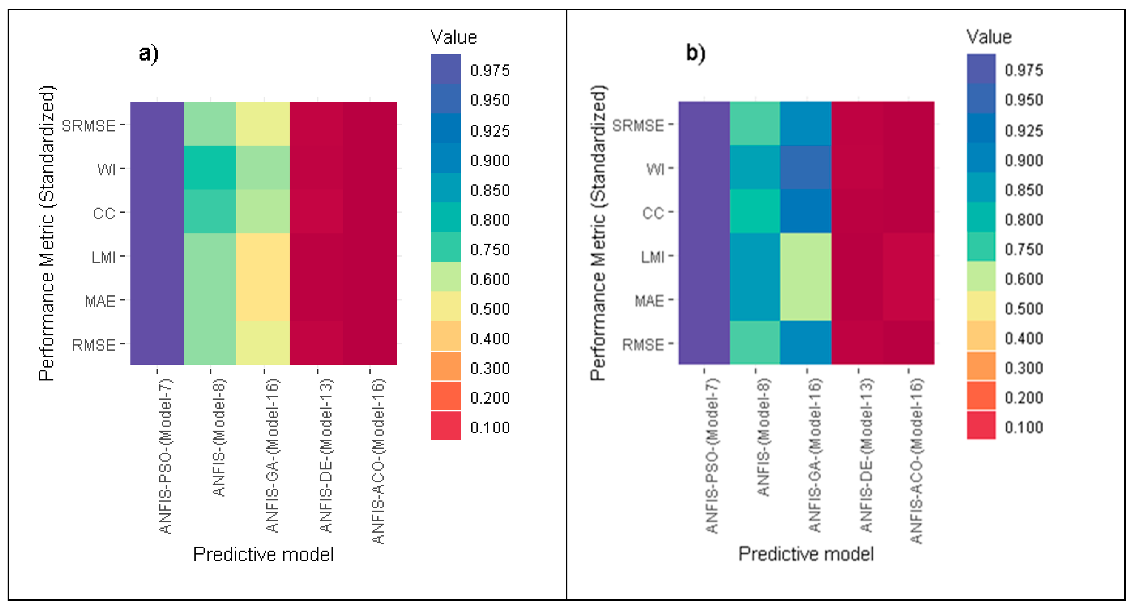
To finalize the best relation between proposed models and the performance metrics, a heat map was created, where this diagram depicts the graphical comparison between models in term of standardized performance indices. It can be seen in Figure 3 that all the standardized performance indices of ANFIS-PSO (Model-7) have a dark blue color (best performance) in both training and testing phases, while ANFIS-ACO (Model-16) appeared to be the lowest in terms of these performance metrics (dark red color).
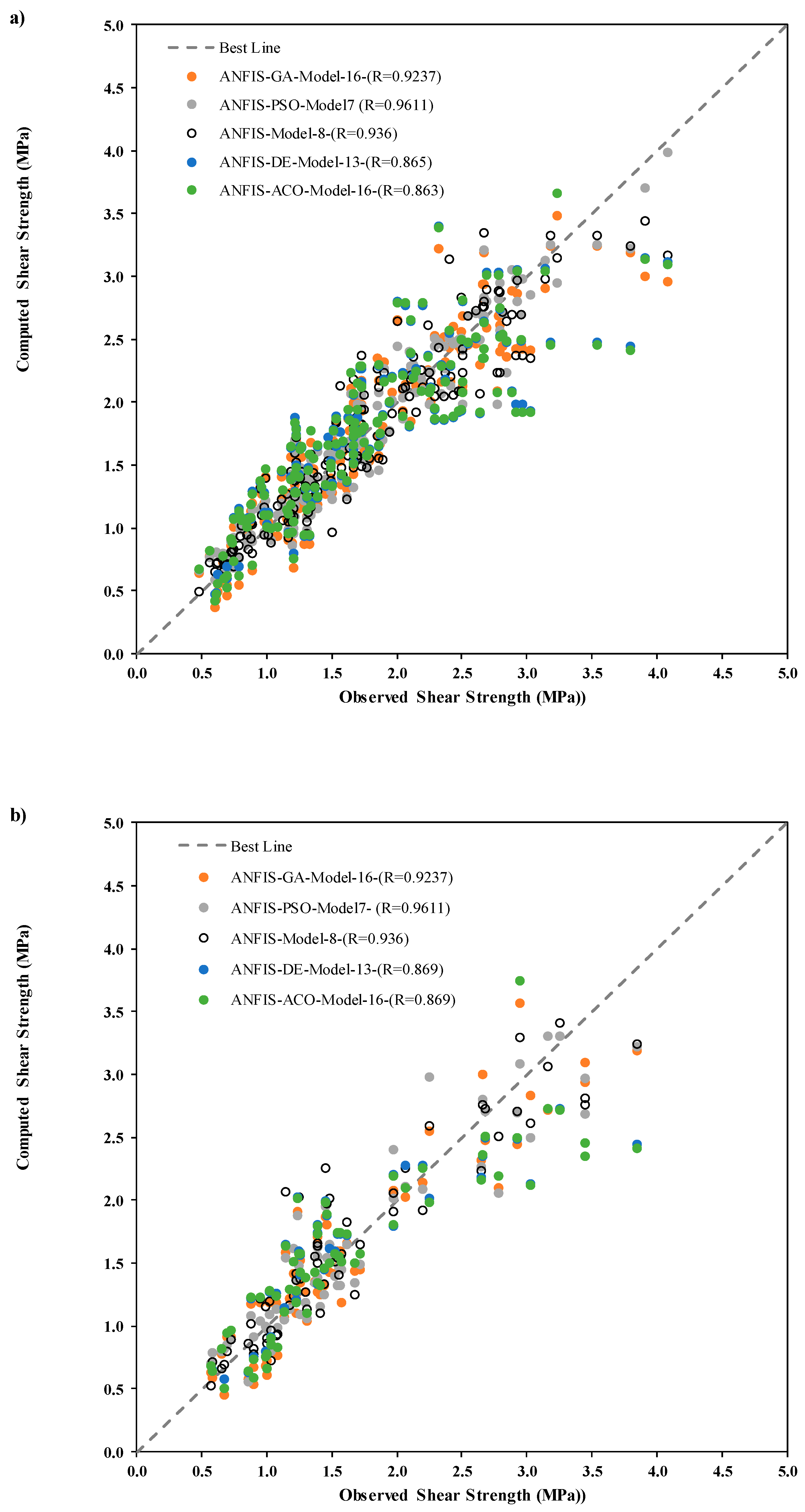
The scatter plots were generated between observed and predicted Ss for the cases of training and testing phases to strengthen the visualization of the applied model’s performance accuracy with the correlation coefficient (R) magnitude (Figure 4). The ANFIS-PSO model was revealed to have better correlation in comparison with the other applied models by achieving higher R value as follows: (ANFIS-PSO ≈ 0.9611, ANFIS ≈ 0.936, ANFIS-GA ≈ 0.9237, ANFIS-DE ≈ 0.865, ANFIS-ACO ≈ 0.863) in training phase and (ANFIS-PSO ≈ 0.9611, ANFIS ≈ 0.936, ANFIS-GA ≈ 0.9237, ANFIS-DE ≈ 0.869, ANFIS-ACO ≈ 0.869) in the testing phase.
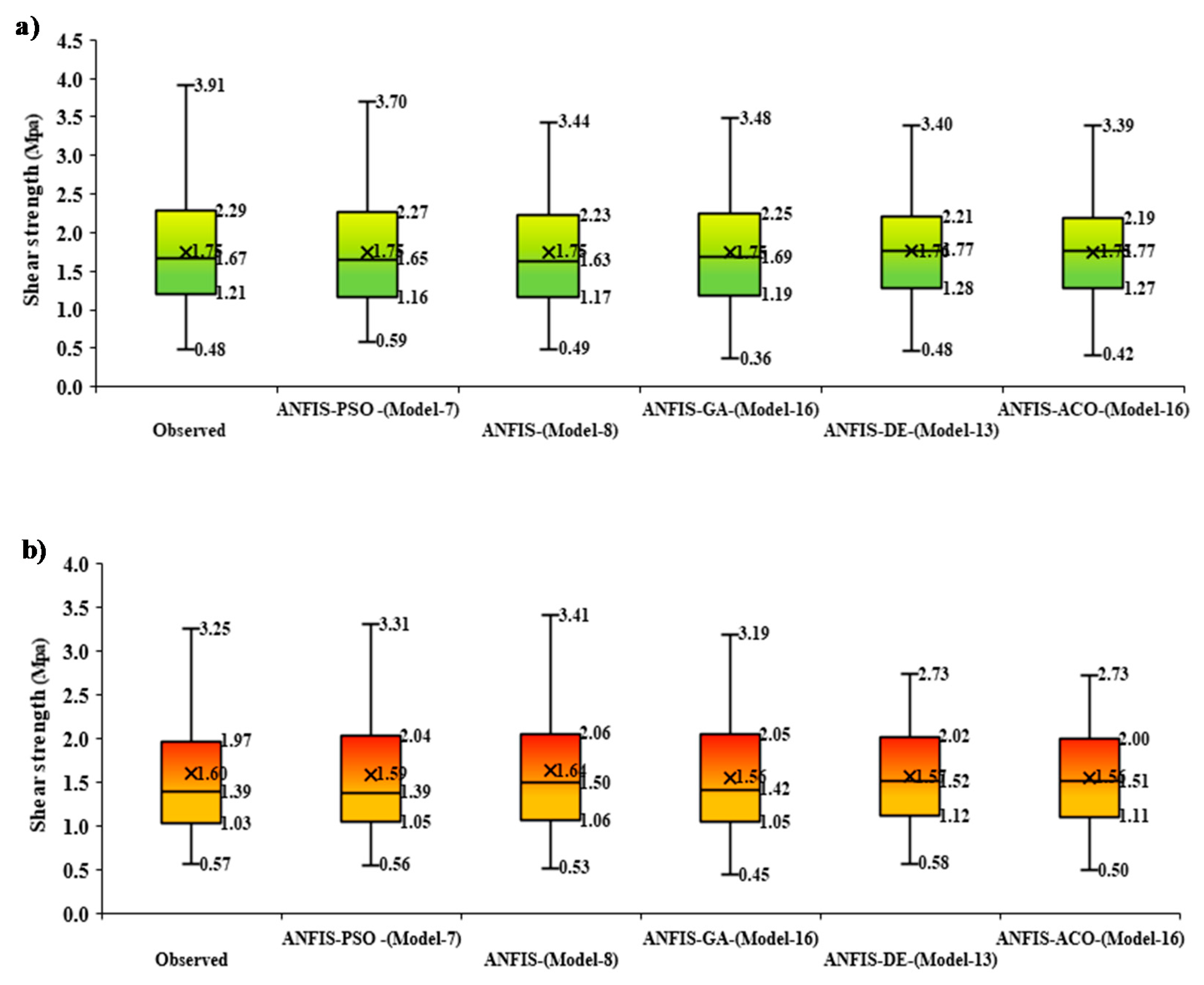
To establish the relationship of the interquartile range (IQR) between observed and predicted Ss by various proposed models, the boxplots of both training (yellow) and testing (green) phases were displayed in Figure 5. The distinction of performances is visible since the prediction was generated via ANFIS-PSO (Model-7) against observed (experimental) Ss, which were significantly accurate in comparison with ANFIS (Model-8), ANFIS-GA (Model-16), ANFIS-DE (Model-13), and ANFIS-ACO (Model-16). Hence, the boxplots, together with the benchmark models against observed Ss, ascertain the better accuracy of ANFIS-PSO model.
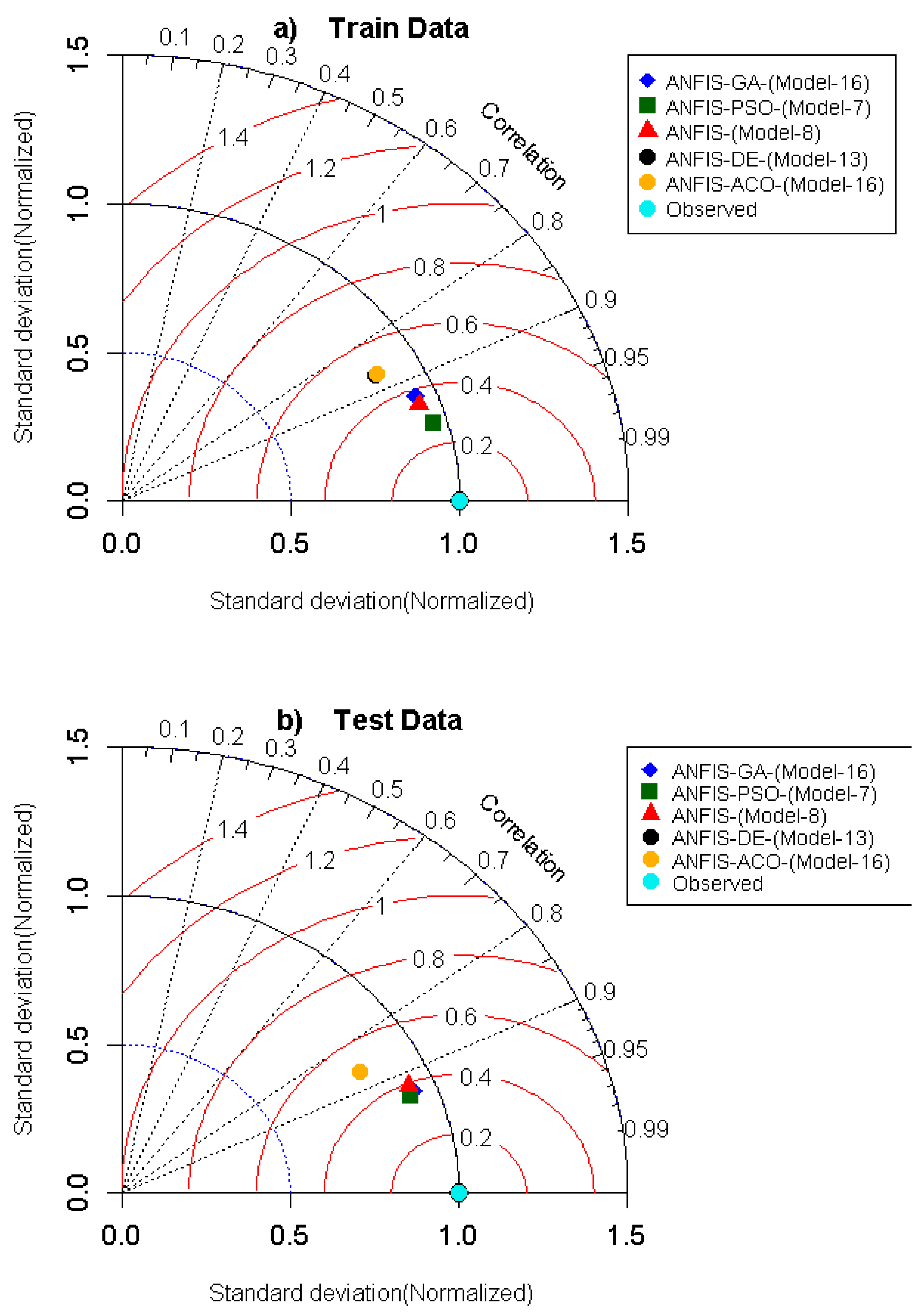
To scale the degree between predicted and experimental Ss of HSC for all proposed hybrid and standalone ANFIS models, a Taylor diagram was drawn (Figure 6). The magnitudes of correlation are shown in the form of the Taylor diagram that generates a more detailed appraisal of the model performances [101] for training and testing phases. The Taylor diagram illustrates a more tangible and convincing statistical relationship between the predicted and observed Ss depending on correlation with respect to standard deviations. It is seen that the benchmark models ANFIS-DE and ANFIS-ACO are not appropriate in the training session, as the correlation to standard deviation points was highly parted from the ideal observed point as compared to ANFIS-PSO, ANFIS, and ANFIS-GA. The hybrid ANFIS-PSO model lay close to the perfect observed point in the testing phase more closely, followed by ANFIS-GA, ANFIS, ANFI-DE, and ANFIS-ACO models, which confirms that the prediction accuracy of ANFS-PSO was reasonably higher than the benchmark models.
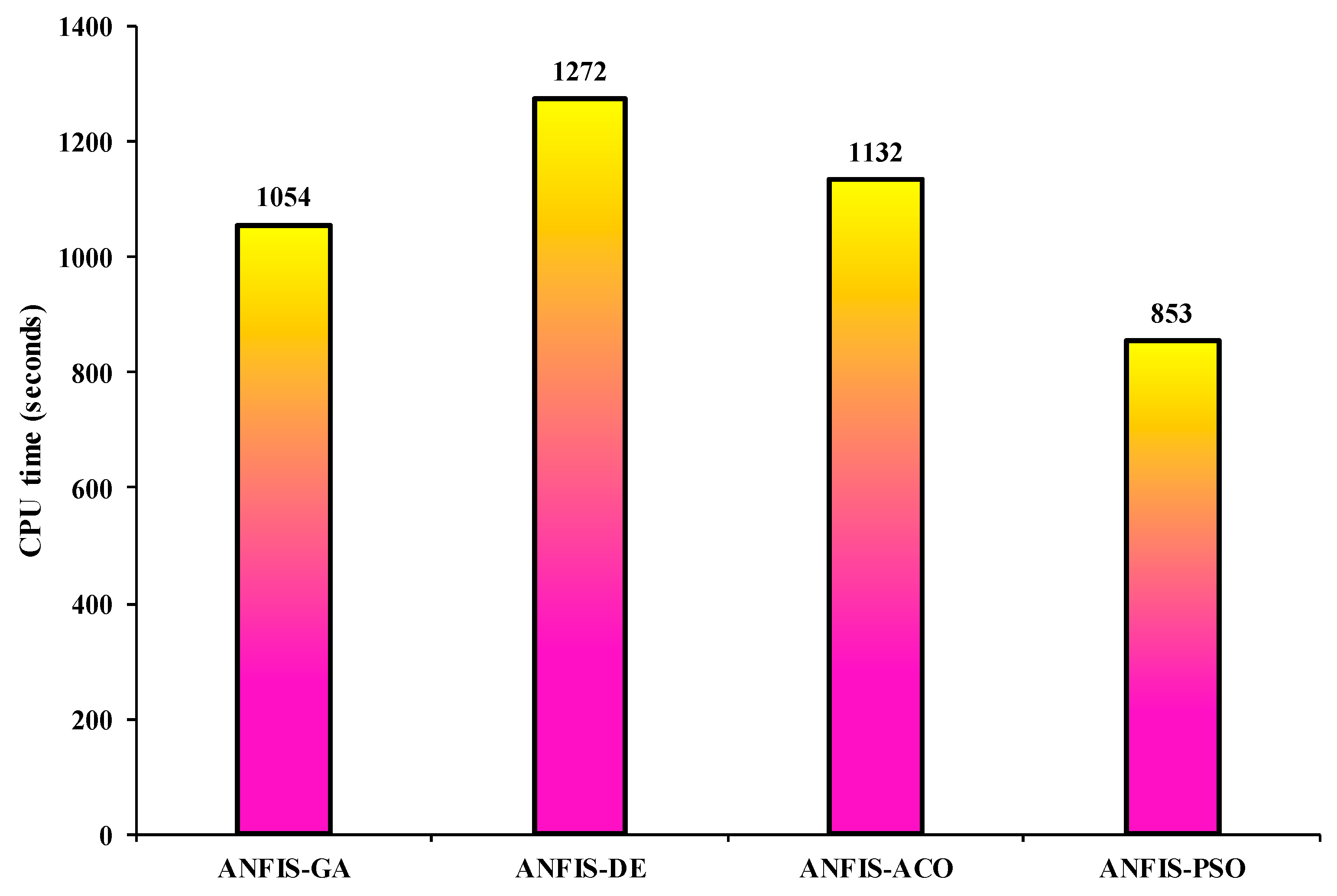
To evaluate the trade-off between the accuracy and efficiency of the newly developed models, their computational time (CPU time) is presented in Figure 7.
From Figure 7, it is evident that the lowest CPU time (853.23 s) is observed in ANFIS-PSO, while the ANFIS-DE offers the highest value (1272.06 s). The results confirm that the ANFIS-PSO model provides the highest performance prediction with most top convergence speed in comparison with other hybrid techniques.
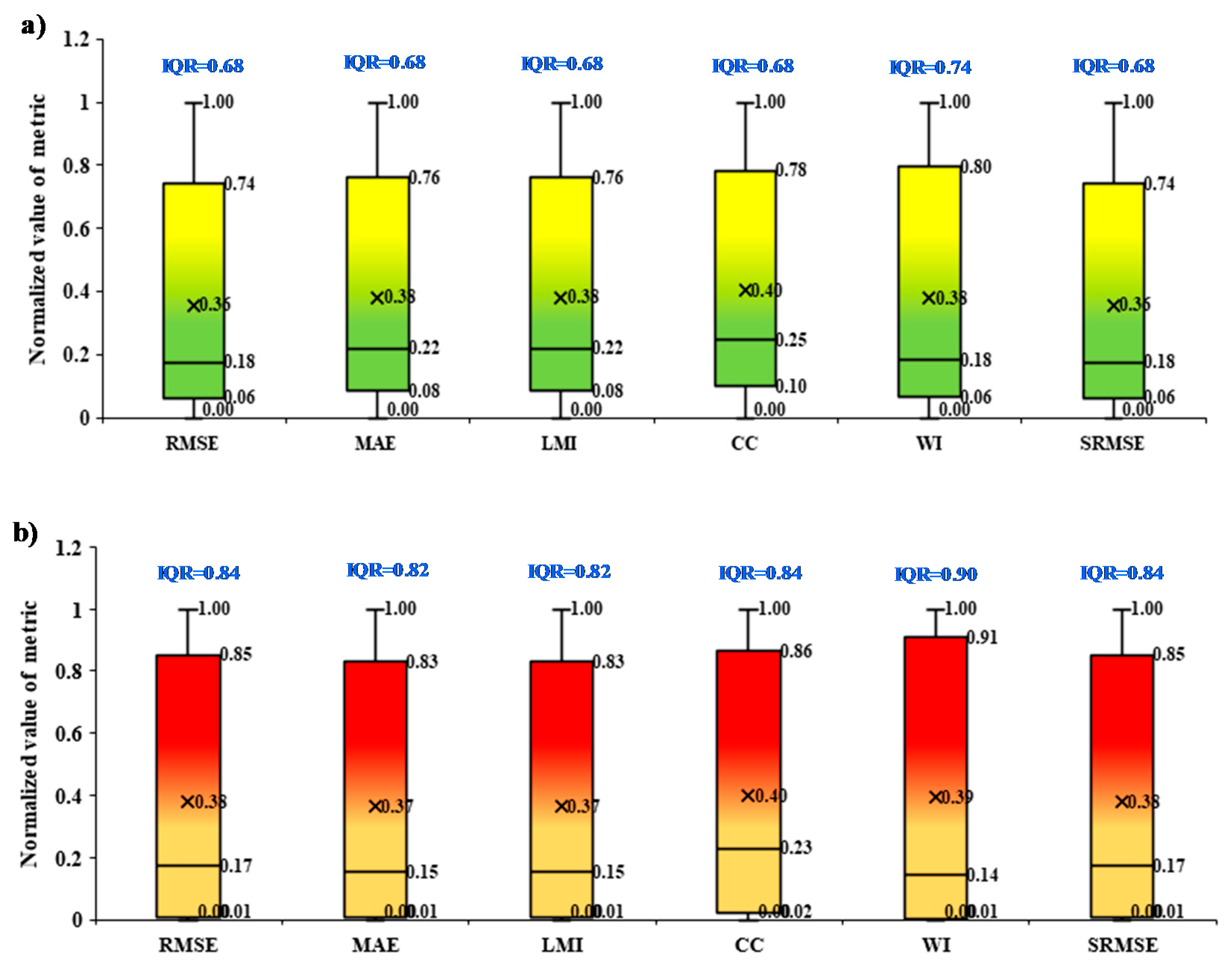
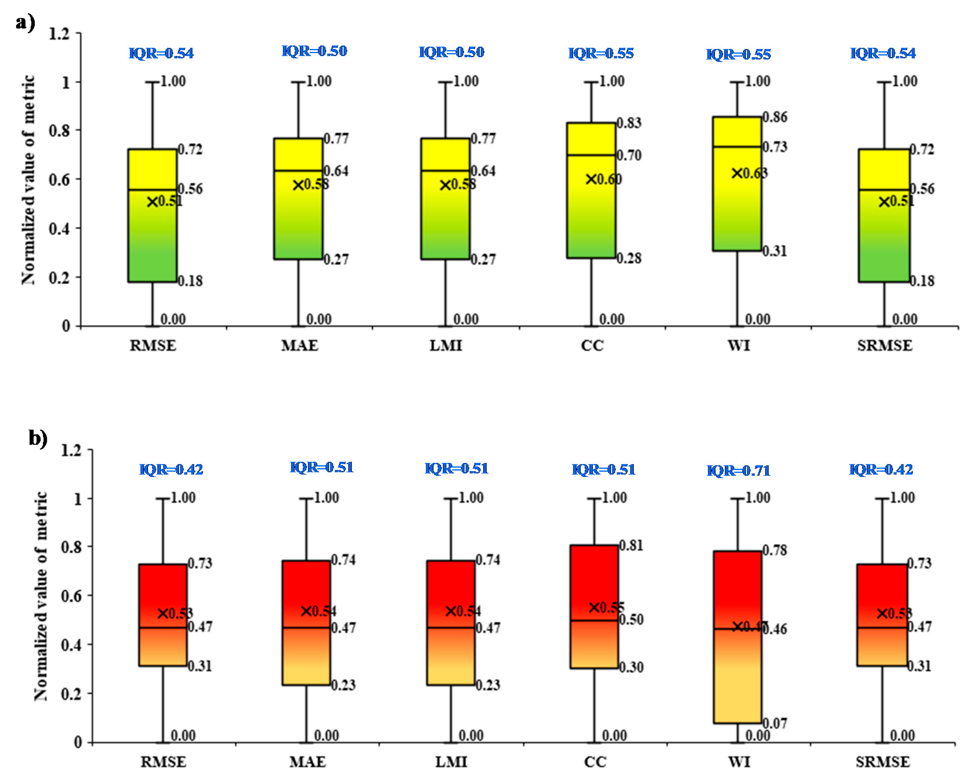
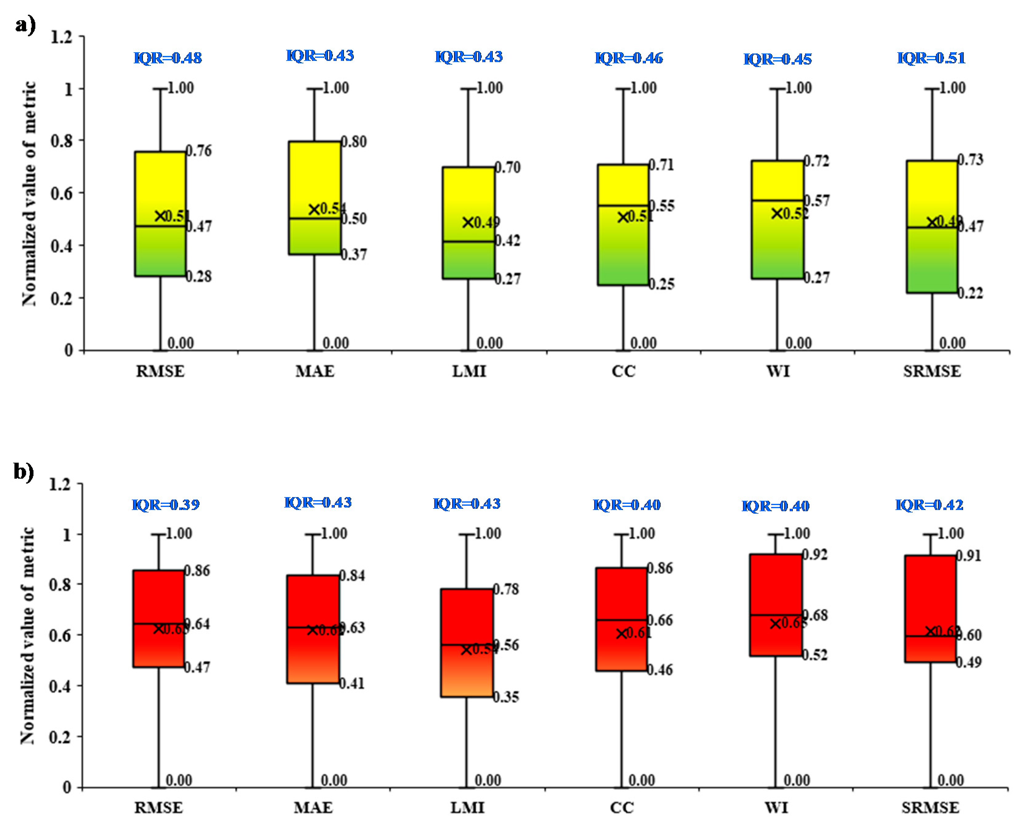
The uncertainties of model, variables, and data were evaluated on the basis of boxplots presentation based on the performance metrics over the training and testing phases at 25%, 50%, and 75% quantile together with IQR (Figured 8, 9, and 10). In the cases of the model’s uncertainty based on performance metrics over the training and testing phases, the majority of the cases revealed a median value towards the 1st quartile for both training and testing phases (Figure 8). However, in the case of the training set, all performance metrics exhibited marginal higher redundant than testing phase with the average values of IQR lies at 0.68 and 0.84, respectively. In cases of variable’s uncertainty based on performance metrics over the training and testing phases were exhibited the distinguished characters (Figure 9); during the training phase, the median value tends towards the 3rd quartile in most of the performance metrics. In contrast, it was mixed, tending towards the 1st quartile (for RMSE, CC, and SRMSE), 2nd quartile (for MAE and LMI), and 3rd quartile (for WI) in the testing phase. In the cases of the data’s uncertainty based on performance metrics over the training and testing phases were presented mixed characteristics such as the median line of boxplot tends towards 1st quartile for RMSE, MAE and LMI, whereas CC and WI were opposite towards the 3rd quartile but remained almost in the middle position in case of SRMSE (Figure 10). However, the testing phase has demonstrated the stability, which is near the middle for all performance metrics except WI and SRMSE, which were towards the 1st quartile.
The aptness of the hybrid and standalone ANFIS models using different input combinations (Model-1, Model-2… Model-18) to predict Ss was explored in this paper. The accuracy of the hybrid ANFIS-PSO with input combination (Model-7) was reasonably superior to the other models (i.e., ANFIS-ACO, ANFIS-GA, ANFIS-DE, and ANFIS) with different combinations of inputs (Table 2, Table 3, Table 4, Table 5 and Table 6), demonstrating that the ANFIS-PSO was a well-designed algorithm to extract pertinent features for Ss prediction. The precision of ANFIS-PSO with other algorithms revealed that the different input combinations were also advantageous in indicating the pertinent features making the model parsimonious.
Since the fundamental operations of the AI models of machine learning are significantly contingent upon the patterns in historical datasets that can substantially disturb the learning strategy, the results here assured the suitability of input combinations to sort out the best combination capturing minimum pertinent features and characteristics. Prior to the prediction process, several input combinations are constructed using related physical properties. The Ss of the HSC slender beams was predicted using two different modeling scenarios based on (i) non-processed (initial) dataset (NP) (i.e., Model-1, Model-2, …, Model-6) and (ii) pre-processed dataset (PP) (i.e., Model-7, Model-8, …, Model-18). This was to examine the influence of the non-homogeneity of the dataset on model prediction accuracy. Apparently, the PP data were excellent data cleaning prior to the model’s construction. This is due to the fact that some redundant measures associated with some error can influence the learning process, which leads to poor predictability capacity.
Based on the attained modeling results, a couple limitations are observed, which are worth to be highlighted for future research. The investigated computer aid model’s performance can be inspected based on the changes in the type of aggregated consideration and evaluating the weight of the interlock strength of the total shear strength. Besides, this is clear, noting that the impact of high strength beam was reported successfully. However, the impact of normal beam shear strength could be a prospective objective. Further, the lateral stability of the slender beam can be investigated, which is totally dependent upon the data availability of the experiments.

4. Conclusions

A contemporary AI model established the prediction of the shear strength of HSC slender beam. The efficiencies of several optimization algorithms (ACO, DE, GA, and PSO) were reported along with pre-processed and non-processed data modeling scenarios. Those modeling scenarios were investigated for the possibility to enhance the prediction accuracy of the applied predictive models. Among all the optimization algorithms, PSO showed the best optimizer for the current intensive dataset in case of pre-processed variables (d, a, ag, fc, and ρ) (excluding a/d and ag/d) as depicted by the performance metrics such as R = 0.9611; RMSE = 0.206; MAE = 0.157; CC = 0.961; WI = 0.980. The IQR characteristic of the dataset between the observed and predicted Ss using ANFIS-PSO exhibited significant similarity. It is clearly visible that the selected pre-processed data alleviate the performance of the hybrid model remarkably. There is need for a prospective study where a lesser exploratory data analysis (EDA) process along with a homogeneous large dataset, with or without a pre-processed dataset, might achieve the best prediction accuracy using the proposed hybrid AI model. In the case in which the performance does maintain a stable result for the non-monotonous IQR dataset, there is a possible prospective study objective to use more derivative data from the primary character of Ss for another either HSC or medium strength concrete.

Author Contributions

Conceptualization, Z.M.Y., A.S., and N.A.-A.; data curation, A.S.; formal analysis, Z.M.Y., M.S.A., M.H.M., A.W.A.Z., M.A., and S.K.B.; investigation, Z.M.Y., M.H., M.S.A., M.H.M., A.W.A.Z., M.A., and N.A.-A.; methodology, A.S. and M.H.; project administration, Z.M.Y.; software, A.S. and M.H.; supervision, Z.M.Y. and N.A.-A.; validation, Z.M.Y., A.S., M.S.A., M.H.M., A.W.A.Z., M.A., and N.A.-A.; visualization, Z.M.Y., M.S.A., M.H.M., A.W.A.Z., and S.K.B.; writing—original draft, Z.M.Y., A.S., M.H., M.S.A., M.H.M., A.W.A.Z., M.A., S.K.B., and N.A.-A.; writing—review and editing, Z.M.Y., A.S., A.W.A.Z., and N.A.-A. All authors have read and agreed to the published version of the manuscript.

Funding

This research received no external funding.

Conflicts of Interest

The authors declare no conflict of interest.

References

  1. Subramanian, N. Evaluation and enhancing the punching shear resistance of flat slabs using HSC. Indian Concr. J. 2005, 79, 31–37. [Google Scholar]
  2. Cuenca, E.; Serna, P. Failure modes and shear design of prestressed hollow core slabs made of fiber-reinforced concrete. Compos. Part B Eng. 2013. [Google Scholar] [CrossRef]
  3. ACI (American Concrete Institute). Report on High Strength Concrete; Aci 363r-10; ACI (American Concrete Institute): Farmington Hills, MI, U.S.A, 2010. [Google Scholar]
  4. Hamrat, M.; Boulekbache, B.; Chemrouk, M.; Amziane, S. Shear Behaviour of RC Beams without Stirrups Made of Normal Strength and High Strength Concretes. Adv. Struct. Eng. 2010, 13, 29–41. [Google Scholar] [CrossRef]
  5. Gebreyouhannes, E.; Maekawa, K. Numerical Simulation on Shear Capacity and Post-Peak Ductility of Reinforced High-Strength Concrete Coupled with Autogenous Shrinkage. J. Adv. Concr. Technol. 2011, 9, 73–88. [Google Scholar] [CrossRef] [Green Version]
  6. Taylor, H.P.J. The fundamental behavior of reinforced concrete beams in bending and shear. Spec. Publ. 1974, 42, 43–78. [Google Scholar] [CrossRef]
  7. Sarkar, S.; Adwan, O.; Bose, B. Shear stress contributions and failure mechanisms of high strengh reinforced concrete beams. Mater. Struct. 2006, 32, 112. [Google Scholar] [CrossRef]
  8. Gandomi, A.H.; Alavi, A.H.; Kazemi, S.; Gandomi, M. Formulation of shear strength of slender RC beams using gene expression programming, part I: Without shear reinforcement. Autom. Constr. 2014, 42, 112–121. [Google Scholar] [CrossRef]
  9. Taylor, H.P.J. Investigation of the Forces Carried Across Cracks in Reinforced Concrete Beams in Shear by Interlock of Aggregate; Cement and Concrete Association: London, UK, 1970. [Google Scholar]
  10. Mphonde, A.G. Aggregate interlock in high strength reinforced concrete beams. Proc. Inst. Civ. Eng. 1988, 85, 397–413. [Google Scholar] [CrossRef]
  11. Kim, J.K.; Park, Y.D. Prediction of shear strength of reinforced concrete beams without web reinforcement. ACI Mater. J. 1996, 93, 213–222. [Google Scholar]
  12. Kaveh, A.; Bakhshpoori, T.; Hamze-Ziabari, S.M. Development of predictive models for shear strength of HSC slender beams without web reinforcement using machine-learning based techniques. Sci. Iran. 2019, 26, 709–725. [Google Scholar] [CrossRef] [Green Version]
  13. Ahmad, S.; Bhargava, P. Shear strength models for reinforced concrete slender beams: A comparative study. In Structures; Elsevier: Amsterdam, The Netherlands, 2018; Volume 16, pp. 119–128. [Google Scholar]
  14. Okamura, H.; Higai, T. Proposed design equation for shear strength of reinforced concrete beams without web reinforcement. In Proceedings of the Japan Society of Civil Engineers; Japan Society of Civil Engineers: Tokyo, Japan, 1980; Volume 1980, pp. 131–141. [Google Scholar]
  15. Adhikary, B.B.; Mutsuyoshi, H. Prediction of shear strength of steel fiber RC beams using neural networks. Constr. Build. Mater. 2006, 20, 801–811. [Google Scholar] [CrossRef]
  16. Adeli, H. Neural networks in civil engineering: 1989–2000. Comput.—Aided Civ. Infrastruct. Eng. 2001, 16, 126–142. [Google Scholar] [CrossRef]
  17. Davoudi, R.; Miller, G.R.; Kutz, J.N. Data-driven vision-based inspection for reinforced concrete beams and slabs: Quantitative damage and load estimation. Autom. Constr. 2018. [Google Scholar] [CrossRef]
  18. Sharafati, A.; Haghbin, M.; Motta, D.; Yaseen, Z.M. The Application of Soft Computing Models and Empirical Formulations for Hydraulic Structure Scouring Depth Simulation: A Comprehensive Review, Assessment and Possible Future Research Direction. Arch. Comput. Methods Eng. 2019, 1–25. [Google Scholar] [CrossRef]
  19. Salih, S.Q.; Sharafati, A.; Khosravi, K.; Faris, H.; Kisi, O.; Tao, H.; Ali, M.; Yaseen, Z.M. River suspended sediment load prediction based on river discharge information: Application of newly developed data mining models. Hydrol. Sci. J. 2019. just accepted. [Google Scholar] [CrossRef]
  20. Malik, A.; Kumar, A.; Kim, S.; Kashani, M.H.; Karimi, V.; Sharafati, A.; Ghorbani, M.A.; Al-Ansari, N.; Salih, S.Q.; Yaseen, Z.M. Modeling monthly pan evaporation process over the Indian central Himalayas: Application of multiple learning artificial intelligence model. Eng. Appl. Comput. Fluid Mech. 2020, 14, 323–338. [Google Scholar] [CrossRef] [Green Version]
  21. Oreta, A.W.C. Simulating size effect on shear strength of RC beams without stirrups using neural networks. Eng. Struct. 2004, 26, 681–691. [Google Scholar] [CrossRef]
  22. Choi, K.-K.; Sherif, A.G.; Taha, M.M.R.; Chung, L. Shear strength of slender reinforced concrete beams without web reinforcement: A model using fuzzy set theory. Eng. Struct. 2009, 31, 768–777. [Google Scholar] [CrossRef]
  23. Cladera, A.; Marí, A.R. Shear design procedure for reinforced normal and high-strength concrete beams using artificial neural networks. Part I: Beams without stirrups. Eng. Struct. 2004, 26, 917–926. [Google Scholar] [CrossRef]
  24. Cladera, A.; Marí, A.R. Shear design procedure for reinforced normal and high-strength concrete beams using artificial neural networks. Part II: Beams with stirrups. Eng. Struct. 2004, 26, 927–936. [Google Scholar] [CrossRef]
  25. Perera, R.; Barchín, M.; Arteaga, A.; Diego, A. De Prediction of the ultimate strength of reinforced concrete beams FRP-strengthened in shear using neural networks. Compos. Part B Eng. 2010, 41, 287–298. [Google Scholar] [CrossRef]
  26. Pal, M.; Deswal, S. Support vector regression based shear strength modelling of deep beams. Comput. Struct. 2011. [Google Scholar] [CrossRef]
  27. Keshtegar, B.; Bagheri, M.; Yaseen, Z.M. Shear strength of steel fiber-unconfined reinforced concrete beam simulation: Application of novel intelligent model. Compos. Struct. 2019, 212, 230–242. [Google Scholar] [CrossRef]
  28. Çevik, A.; Kurtoğlu, A.E.; Bilgehan, M.; Gülşan, M.E.; Albegmprli, H.M. Support vector machines in structural engineering: A review. J. Civ. Eng. Manag. 2015, 21, 261–281. [Google Scholar] [CrossRef]
  29. Ashrafian, A.; Shokri, F.; Amiri, M.J.T.; Yaseen, Z.M.; Rezaie-Balf, M. Compressive strength of Foamed Cellular Lightweight Concrete simulation: New development of hybrid artificial intelligence model. Constr. Build. Mater. 2020, 230, 117048. [Google Scholar] [CrossRef]
  30. Ashour, A.F.; Alvarez, L.F.; Toropov, V.V. Empirical modelling of shear strength of RC deep beams by genetic programming. Comput. Struct. 2003. [Google Scholar] [CrossRef]
  31. Gandomi, A.H.; Alavi, A.H.; Yun, G.J. Nonlinear modeling of shear strength of {SFRC} beams using linear genetic programming. Struct. Eng. Mech. Int. J. 2011, 38, 1–25. [Google Scholar] [CrossRef]
  32. Kara, I.F. Prediction of shear strength of FRP-reinforced concrete beams without stirrups based on genetic programming. Adv. Eng. Softw. 2011. [Google Scholar] [CrossRef]
  33. Gandomi, A.H.; Yun, G.J.; Alavi, A.H. An evolutionary approach for modeling of shear strength of RC deep beams. Mater. Struct. 2013, 46, 2109–2119. [Google Scholar] [CrossRef]
  34. Mansouri, I.; Shariati, M.; Safa, M.; Ibrahim, Z.; Tahir, M.M.; Petković, D. Analysis of influential factors for predicting the shear strength of a V-shaped angle shear connector in composite beams using an adaptive neuro-fuzzy technique. J. Intell. Manuf. 2019. [Google Scholar] [CrossRef]
  35. Amani, J.; Moeini, R. Prediction of shear strength of reinforced concrete beams using adaptive neuro-fuzzy inference system and artificial neural network. Sci. Iran. 2012, 19, 242–248. [Google Scholar] [CrossRef] [Green Version]
  36. Nasrollahzadeh, K.; Basiri, M.M. Prediction of shear strength of FRP reinforced concrete beams using fuzzy inference system. Expert Syst. Appl. 2014. [Google Scholar] [CrossRef]
  37. Safa, M.; Shariati, M.; Ibrahim, Z.; Toghroli, A.; Baharom, S.B.; Nor, N.M.; Petkovic, D. Potential of adaptive neuro fuzzy inference system for evaluating the factors affecting steel-concrete composite beam’s shear strength. Steel Compos. Struct. 2016. [Google Scholar] [CrossRef]
  38. Toghroli, A.; Mohammadhassani, M.; Suhatril, M.; Shariati, M.; Ibrahim, Z. Prediction of shear capacity of channel shear connectors using the ANFIS model. Steel Compos. Struct. 2014. [Google Scholar] [CrossRef]
  39. Adoko, A.C.; Wu, L. Fuzzy inference systems-based approaches in geotechnical engineering—A review. Electron. J. Geotech. Eng. 2011, 16, 1543–1558. [Google Scholar]
  40. Sharafati, A.; Tafarojnoruz, A.; Shourian, M.; Yaseen, Z.M. Simulation of the depth scouring downstream sluice gate: The validation of newly developed data-intelligent models. J. Hydro-Environ. Res. 2019, 29, 20–30. [Google Scholar] [CrossRef]
  41. Mohammed, M.; Sharafati, A.; Al-Ansari, N.; Yaseen, Z.M. Shallow Foundation Settlement Quantification: Application of Hybridized Adaptive Neuro-Fuzzy Inference System Model. Adv. Civ. Eng. 2020, 2020, 7381617. [Google Scholar] [CrossRef] [Green Version]
  42. Mottahedi, A.; Sereshki, F.; Ataei, M. Overbreak prediction in underground excavations using hybrid ANFIS-PSO model. Tunn. Undergr. Space Technol. 2018. [Google Scholar] [CrossRef]
  43. Karaboga, D.; Kaya, E. An adaptive and hybrid artificial bee colony algorithm (aABC) for ANFIS training. Appl. Soft Comput. J. 2016. [Google Scholar] [CrossRef]
  44. Nguyen, D.T.; Yin, S.; Tang, Q.; Son, P.X.; Duc, L.A. Online monitoring of surface roughness and grinding wheel wear when grinding Ti-6Al-4V titanium alloy using ANFIS-GPR hybrid algorithm and Taguchi analysis. Precis. Eng. 2019. [Google Scholar] [CrossRef]
  45. Mozdgir, A.; Mahdavi, I.; Badeleh, I.S.; Solimanpur, M. Using the Taguchi method to optimize the differential evolution algorithm parameters for minimizing the workload smoothness index in simple assembly line balancing. Math. Comput. Model. 2013, 57, 137–151. [Google Scholar] [CrossRef]
  46. Shah, A.; Ahmad, S. An experimental investigation into shear capacity of high strength concrete beams. Asian J. Civil Eng. (Build. Hous.) 2007, 8, 549–562. [Google Scholar]
  47. Collins, M.; Kuchma, D. How safe are our large, lightly reinforced concrete beams, slabs, and footings? Struct. J. 1999, 96, 482–490. [Google Scholar]
  48. Elzanaty, A.; Nilson, A.; Slate, F. Shear Capacity of Reinforced Concrete Beams Using High-Strength Concrete. ACI J. Proc. 1986, 83. [Google Scholar] [CrossRef]
  49. Al-Shaleh, K.; Rahal, K.N. Shear behavior of K850 reinforced concrete beams with low transverse reinforcement. Kuwait J. Sci. Eng. 2007, 34, 35. [Google Scholar]
  50. Sagaseta, J.; Vollum, R.L. Non-linear finite element analysis of shear critical high strength concrete beams. Archit. Civ. Eng. Environ.—ACEE 2009, 2, 95–106. [Google Scholar]
  51. Eisa, A.S.A. Shear strength of high strength concrete beams. Master’s Thesis, Zagazig University, Zagazig, Egypt, 2005. [Google Scholar]
  52. Ahmad, S.H.; Khaloo, A.R.; Poveda, A. Shear capacity of reinforced high-strength concrete beams. J. Proc. 1986, 83, 297–305. [Google Scholar]
  53. Jin-Keun, K.; Yon-Dong, P. Shear strength of reinforced high strength concrete beam without web reinforcement. Mag. Concr. Res. 1994, 46, 7–16. [Google Scholar] [CrossRef]
  54. Moustafa, M.T. Behaviour of high strength concrete beams. Struct. Concr. 1999, 4, 175–183. [Google Scholar]
  55. Mphonde, A.G.; Frantz, G.C. Shear Tests of High- and Low-Strength Concrete Beams without Stirrups. ACI J. Proc. 1984, 81. [Google Scholar] [CrossRef]
  56. Pendyala, R.; Mendis, P. Experimental Study on Shear Strength of High-Strength Concrete Beams. ACI Struct. J. 2000, 97. [Google Scholar] [CrossRef]
  57. Shin, S.; Lee, K.; Moon, J.; Ghosh, S. Shear Strength of Reinforced High-Strength Concrete Beams with Shear Span-to-Depth Ratios between 1.5 and 2.5. ACI Struct. J. 1999, 96, 549–556. [Google Scholar]
  58. Yoon, Y.; Cook, W.; Mitchell, D. Minimum Shear Reinforcement in Normal, Medium, and High-Strength Concrete Beams. ACI Struct. J. 1996, 93, 576–584. [Google Scholar]
  59. Xie, Y.; Ahmad, S.; Yu, T.; Hino, S.; Chung, W. Shear Ductility of Reinforced Concrete Beams of Normal and High-Strength Concrete. Aci Struct. J. 1994, 91, 140–149. [Google Scholar]
  60. Cladera, A.; Marí, A.R. Experimental study on high-strength concrete beams failing in shear. Eng. Struct. 2005, 27, 1519–1527. [Google Scholar] [CrossRef]
  61. Perera, S.; Mutsuyoshi, H. Shear Behavior of Reinforced High-Strength Concrete Beams. ACI Struct. J. 2013, 110. [Google Scholar] [CrossRef]
  62. Ali, S. Flexural and Shear Behavior of High-Strength Concrete Beams. Master’s Thesis, University of Engineering & Technology, Taxila, Pakistan, 2001. [Google Scholar]
  63. Grimm, R. Influence of Fracture Mechanics Parameters on the Bending and Shear Bearing Behavior of Highstrength Concretes. Ph.D. Thesis, Construction Engineering of the Technical University of Darmstadt, Berlin, Germany, 1997. [Google Scholar]
  64. Hallgren, M. Flexural and Shear Capacity of Reinforced High Strength Concrete Beams without Stirrups.; TRITABKN. Bull.9; Department of Structural Engineering, Royal Institute of Technology: Stockholm, Sweden, 1994; pp. 1–49. [Google Scholar]
  65. Podgorniak-Stanik, B.A. The Influence of Concrete Strength, Distribution of Longitudinal Reinforcement, Amount of Transverse Reinforcement and Member Size on Shear Strength of Reinforced Concrete Members. Master’s Thesis, University of Toronto, Toronto, ON, Canada, 1998. [Google Scholar]
  66. Morrow, J.; Viest, I. Shear Strength of Reinforced Concrete Frame Members without Web Reinforcement. ACI J. Proc. 1957, 53. [Google Scholar] [CrossRef]
  67. Remmel, G. For Tensile Behavior of High-Strength Concrete and Its Influence on the Shear Capacity of Slender Members without Shear Reinforcement. Ph.D. Thesis, Construction Engineering of the Technical University of Darmstadt, Berlin, Germany, 1991. [Google Scholar]
  68. Scholz, H. A Lateral Force Support Model for Components without Shear Reinforcement at Failure of Normal Strength and High Strength Concrete; Reports from the Structural Engineering Bulletin 21; Technical University of Berlin: Berlin, Germany, 1994. [Google Scholar]
  69. Drangsholt, G.; Thorenfeldt, E. High Strength Concrete. SP2—Plates and Shells. Report 2.1, Shear Capacity of High Strength Concrete Beams; SINTEF Structures and Concrete: Trondheim, Norway, 1992. [Google Scholar]
  70. Angelakos, D.; Bentz, E.; Mp, C. Effect of Concrete Strength and Minimum Stirrups on Shear Strength of Large Members. ACI Struct. J. 2001, 98. [Google Scholar] [CrossRef]
  71. Adebar, P.; Collins, M.P. Shear strength of members without transverse reinforcement. Can. J. Civ. Eng. 1996, 23, 30–41. [Google Scholar] [CrossRef]
  72. Salandra, M.; Ahmad, S. Shear Capacity of Reinforced Lightweight High-Strength Concrete Beams. ACI Struct. J. 1989, 86. [Google Scholar] [CrossRef]
  73. Islam, M.S.; Pam, H.J.; Kwan, A.K.H. Shear capacity of high-strength concrete beams with their point of inflection within the shear span. Proc. Inst. Civ. Eng.—Struct. Build. 1998, 128, 91–99. [Google Scholar] [CrossRef] [Green Version]
  74. Kulkarni, S.; Shah, S. Response of Reinforced Concrete Beams at High Strain Rates. ACI Struct. J. 1998, 95. [Google Scholar] [CrossRef]
  75. Hallgren, M. Punching Shear Capacity of Reinforced High Strength Concrete Slabsp; KTH Stockholm und TRITA-BKN: Stockholm, Sweden, 1996. [Google Scholar]
  76. Hanson, J. Tensile Strength and Diagonal Tension Resistance of Structural Lightweight Concrete. ACI J. Proc. 1961, 58. [Google Scholar] [CrossRef]
  77. Bukhari, I.A.; Ahmad, S. Evaluation of shear strength of high-strength concrete beams without stirrups. Arab. J. Sci. Eng. 2008, 33, 321. [Google Scholar]
  78. Abellan-Nebot, J.V.; Subrión, F.R. A review of machining monitoring systems based on artificial intelligence process models. Int. J. Adv. Manuf. Technol. 2009. [Google Scholar] [CrossRef]
  79. Yaseen, Z.; Ebtehaj, I.; Kim, S.; Sanikhani, H.; Asadi, H.; Ghareb, M.; Bonakdari, H.; Wan Mohtar, W.; Al-Ansari, N.; Shahid, S. Novel Hybrid Data-Intelligence Model for Forecasting Monthly Rainfall with Uncertainty Analysis. Water 2019, 11, 502. [Google Scholar] [CrossRef] [Green Version]
  80. Naderpour, H.; Kheyroddin, A.; Amiri, G.G. Prediction of FRP-confined compressive strength of concrete using artificial neural networks. Compos. Struct. 2010. [Google Scholar] [CrossRef]
  81. Naderpour, H.; Alavi, S.A. A proposed model to estimate shear contribution of FRP in strengthened RC beams in terms of Adaptive Neuro-Fuzzy Inference System. Compos. Struct. 2017. [Google Scholar] [CrossRef]
  82. Demir, F. A new way of prediction elastic modulus of normal and high strength concrete-fuzzy logic. Cem. Concr. Res. 2005. [Google Scholar] [CrossRef]
  83. Jang, J.S.R. ANFIS: Adaptive-Network-Based Fuzzy Inference System. IEEE Trans. Syst. Man Cybern. 1993, 23, 665–685. [Google Scholar] [CrossRef]
  84. Fullér, R. Neural Fuzzy Systems; ESF Series A: 443; Abo Akademis Tryckeri: Turku, Finland, 1995; ISBN 9516506240. [Google Scholar]
  85. Eberhart, R.; Kennedy, J. A new optimizer using particle swarm theory. In Proceedings of the Sixth International Symposium on Micro Machine and Human Science, Nagoya, Japan, 4–6 October 1995; pp. 39–43. [Google Scholar]
  86. Shi, Y.; Eberhart, R.C. Empirical study of particle swarm optimization. In Proceedings of the 1999 Congress on Evolutionary Computation-CEC99, Washington, DC, USA, 6–9 July 1999; Volume 3, pp. 1945–1950. [Google Scholar]
  87. Dorigo, M.; Socha, K. Ant colony optimization. IEEE Comput. Intell. Mag. 2006, 1, 28–39. [Google Scholar] [CrossRef]
  88. Dorigo, M.; Di Caro, G. Ant colony optimization: A new meta-heuristic. In Proceedings of the 1999 Congress on Evolutionary Computation, CEC 1999, Washington, DC, USA, 6–9 July 1999. [Google Scholar]
  89. Merkle, D.; Middendorf, M.; Schmeck, H. Ant colony optimization for resource-constrained project scheduling. IEEE Trans. Evol. Comput. 2002. [Google Scholar] [CrossRef] [Green Version]
  90. Storn, R.; Price, K. Differential evolution–a simple and efficient heuristic for global optimization over continuous spaces. J. Glob. Optim. 1997, 341–359. [Google Scholar] [CrossRef]
  91. Price, K.; Storn, R.M.; Lampinen, J.A. Differential Evolution: A Practical Approach to Global Optimization (Natural Computing Series). J. Hered. 2005. [Google Scholar] [CrossRef]
  92. García-Martínez, C.; Rodriguez, F.J.; Lozano, M. Genetic algorithms. In Handbook of Heuristics; Springer: New York, NY, USA, 2018; ISBN 9783319071244. [Google Scholar]
  93. Goldberg, D.E. Genetic algorithms in search, optimization, and machine learning. Choice Rev. Online 2013. [Google Scholar] [CrossRef]
  94. Harik, G.R.; Lobo, F.G.; Goldberg, D.E. The compact genetic algorithm. IEEE Trans. Evol. Comput. 1999. [Google Scholar] [CrossRef] [Green Version]
  95. Shoorehdeli, M.A.; Teshnehlab, M.; Sedigh, A.K. Novel hybrid learning algorithms for tuning ANFIS parameters using adaptive weighted PSO. In Proceedings of the 2007 IEEE International Fuzzy Systems Conference, London, UK, 23–26 July 2007; pp. 1–6. [Google Scholar]
  96. Yang, X.; Magnusson, J.; Xu, C.-Y. Transferability of regionalization methods under changing climate. J. Hydrol. 2019, 568, 67–81. [Google Scholar] [CrossRef]
  97. Al-Musawi, A.A.; Alwanas, A.A.H.; Salih, S.Q.; Ali, Z.H.; Tran, M.T.; Yaseen, Z.M. Shear strength of SFRCB without stirrups simulation: Implementation of hybrid artificial intelligence model. Eng. Comput. 2020, 36, 1–11. [Google Scholar] [CrossRef]
  98. Salih, S.Q.; Sharafati, A.; Ebtehaj, I.; Sanikhani, H.; Siddique, R.; Deo, R.C.; Bonakdari, H.; Shahid, S.; Yaseen, Z.M. Integrative stochastic model standardization with genetic algorithm for rainfall pattern forecasting in tropical and semi-arid environments. Hydrol. Sci. J. 2020, 65, 1145–1157. [Google Scholar] [CrossRef]
  99. Sharafati, A.; Yasa, R.; Azamathulla, H.M. Assessment of stochastic approaches in prediction of wave-induced pipeline scour depth. J. Pipeline Syst. Eng. Pract. 2018, 9. [Google Scholar] [CrossRef]
  100. Hai, T.; Sharafati, A.; Mohammed, A.; Salih, S.Q.; Deo, R.C.; Al-Ansari, N.; Yaseen, Z.M. Global Solar Radiation Estimation and Climatic Variability Analysis Using Extreme Learning Machine Based Predictive Model. IEEE Access 2020, 8, 12026–12042. [Google Scholar] [CrossRef]
  101. Taylor, K.E. Summarizing multiple aspects of model performance in a single diagram. J. Geophys. Res. Atmos. 2001, 106, 7183–7192. [Google Scholar] [CrossRef]
Figure 1. The structure of the adaptive neuro-fuzzy inference system model.
Applsci 10 03811 g001
Figure 2. The flow chart of the proposed hybrid adaptive neuro-fuzzy inference system (ANFIS) model, the optimization procedure of each integrated nature-inspired algorithm.
Applsci 10 03811 g002
Figure 3. Heat map of the applied hybrid predictive models: (a) Training stage and (b) Testing stage.
Applsci 10 03811 g003
Figure 4. Scatter plots presentation between the observed and predicted values of computed shear strength for the best input combination and models: (a) Training stage and (b) Testing stage.
Applsci 10 03811 g004
Figure 5. Boxplot of computed shear strength against predicted ones (a) Training stage and (b) Testing stage.
Applsci 10 03811 g005
Figure 6. Normalized Taylor diagrams of predicted and observed standardized shear strength: (a) Training stage and (b) Testing stage.
Applsci 10 03811 g006
Figure 7. Comparison between computational time (CPU time) obtained from hybrid ANFIS models.
Applsci 10 03811 g007
Figure 8. Boxplot of the model’s uncertainty based on performance index over (a) Training stage and (b) Testing stage.
Applsci 10 03811 g008
Figure 9. Boxplot of variable’s uncertainty based on performances index over (a) Training stage and (b) Testing stage.
Applsci 10 03811 g009
Figure 10. Boxplot of data’s uncertainty based on indices over (a) Training stage and (b) Testing stage.
Applsci 10 03811 g010
Table 1. The input combinations constructed for building the proposed hybrid estimator models for both pre-processed and non-preprocessed dataset.
ModelsDatadaagfcρa/dag/d
Model-1Not Pre-processed--
Model-2Not Pre-processed---
Model-3Not Pre-processed---
Model-4Not Pre-processed---
Model-5Not Pre-processed---
Model-6Not Pre-processed---
Model-7Pre-processed--
Model-8Pre-processed---
Model-9Pre-processed---
Model-10Pre-processed---
Model-11Pre-processed---
Model-12Pre-processed---
Model-13Pre-processed--
Model-14Pre-processed---
Model-15Pre-processed---
Model-16Pre-processed---
Model-17Pre-processed---
Model-18Pre-processed---
Table 2. The prediction performance of the standalone ANFIS model for all proposed input combinations over the training and testing stage. The boldfaced represents the best ANFIS model.
Predictive ModelsInput CombinationStageRMSEMAELMICCWISRMSE
ANFISModel-1Train0.3170.2270.6260.9050.94817.883
ANFISModel-1Test0.4270.3130.4950.8480.91725.706
ANFISModel-2Train0.2980.2200.6390.9170.95516.792
ANFISModel-2Test0.3970.2790.5500.8710.92623.887
ANFISModel-3Train0.3590.2480.5930.8760.93020.221
ANFISModel-3Test1.2210.4860.2160.4390.55873.470
ANFISModel-4Train0.2900.2090.6560.9210.95716.371
ANFISModel-4Test0.4170.3030.5120.8570.92125.088
ANFISModel-5Train0.3300.2450.5970.8960.94318.634
ANFISModel-5Test0.4300.3180.4870.8450.91225.872
ANFISModel-6Train0.4560.3460.4310.7900.87525.730
ANFISModel-6Test0.5370.4180.3250.7480.85132.298
ANFISModel-7Train0.2950.2180.6420.9190.95616.852
ANFISModel-7Test0.3200.2410.6130.9160.95619.936
ANFISModel-8Train0.2630.1980.6750.9360.96615.011
ANFISModel-8Test0.3140.2240.6400.9200.95719.584
ANFISModel-9Train0.3560.2440.5980.8790.93220.321
ANFISModel-9Test1.0760.4260.3160.4770.61467.103
ANFISModel-10Train0.2890.2110.6530.9220.95816.483
ANFISModel-10Test0.3270.2280.6350.9120.95120.403
ANFISModel-11Train0.3080.2300.6230.9110.95117.603
ANFISModel-11Test0.3910.2900.5350.8720.92724.373
ANFISModel-12Train0.4510.3410.4390.7970.87925.787
ANFISModel-12Test0.4810.3800.3900.7980.88129.972
ANFISModel-13Train0.2880.2230.6330.9230.95816.445
ANFISModel-13Test0.3660.2730.5620.8890.93622.811
ANFISModel-14Train0.2970.2290.6230.9180.95516.965
ANFISModel-14Test0.3330.2430.6110.9090.95120.743
ANFISModel-15Train0.3470.2550.5800.8850.93619.849
ANFISModel-15Test0.4150.3150.4940.8610.90925.859
ANFISModel-16Train0.3020.2230.6330.9150.95417.228
ANFISModel-16Test0.3050.2270.6360.9250.95719.045
ANFISModel-17Train0.2840.2150.6460.9250.96016.223
ANFISModel-17Test0.3560.2580.5860.8950.94422.180
ANFISModel-18Train0.4700.3540.4180.7780.86226.841
ANFISModel-18Test0.5050.4020.3550.7770.85931.477
Table 3. The prediction performance of the hybrid ANFIS-ACO model for all proposed input combinations over the training and testing stage. The boldface denotes the best ANFIS-ACO model.
Predictive ModelsInput CombinationStagesRMSEMAELMICCWISRMSE
ANFIS-ACOModel-1Train0.3810.2860.5300.8600.91921.460
ANFIS-ACOModel-1Test0.4140.3070.5050.8590.91424.940
ANFIS-ACOModel-2Train0.3880.2910.5220.8530.91521.889
ANFIS-ACOModel-2Test0.4250.3130.4950.8520.90625.569
ANFIS-ACOModel-3Train0.4180.3140.4840.8280.89823.567
ANFIS-ACOModel-3test0.4670.3550.4270.8170.87928.103
ANFIS-ACOModel-4Train0.3820.2830.5350.8590.91921.525
ANFIS-ACOModel-4Test0.4140.3060.5060.8590.91324.931
ANFIS-ACOModel-5Train0.3900.2890.5250.8520.91422.003
ANFIS-ACOModel-5Test0.4170.3030.5110.8570.91225.092
ANFIS-ACOModel-6Train0.5750.4740.2210.6350.74332.431
ANFIS-ACOModel-6Test0.6480.5220.1580.5990.73738.993
ANFIS-ACOModel-7Train0.3770.2840.5330.8630.92221.557
ANFIS-ACOModel-7Test0.4050.2960.5250.8650.91625.261
ANFIS-ACOModel-8Train0.3860.2890.5250.8560.91722.050
ANFIS-ACOModel-8Test0.4210.3060.5080.8530.90626.274
ANFIS-ACOModel-9Train0.4190.3140.4830.8280.89823.914
ANFIS-ACOModel-9Test0.4770.3670.4110.8040.87229.763
ANFIS-ACOModel-10Train0.3790.2800.5400.8620.92121.659
ANFIS-ACOModel-10Test0.4040.2930.5300.8660.91625.229
ANFIS-ACOModel-11Train0.3830.2850.5310.8590.91921.876
ANFIS-ACOModel-11Test0.4080.2930.5300.8620.91425.465
ANFIS-ACOModel-12Train0.5800.4780.2150.6300.73833.146
ANFIS-ACOModel-12Test0.6020.4870.2190.6550.77037.556
ANFIS-ACOModel-13Train0.3770.2830.5350.8630.92221.552
ANFIS-ACOModel-13Test0.3990.2890.5360.8700.91824.914
ANFIS-ACOModel-14Train0.4180.3060.4970.8290.89823.865
ANFIS-ACOModel-14Test0.4380.3170.4910.8400.89627.338
ANFIS-ACOModel-15Train0.4270.3200.4740.8200.89324.407
ANFIS-ACOModel-15Test0.4780.3660.4130.8070.86629.828
ANFIS-ACOModel-16Train0.3770.2820.5370.8630.92121.563
ANFIS-ACOModel-16Test0.3990.2890.5360.8700.91824.912
ANFIS-ACOModel-17Train0.3840.2860.5300.8580.91821.936
ANFIS-ACOModel-17Test0.4030.2880.5380.8660.91625.162
ANFIS-ACOModel-18Train0.5810.4770.2150.6300.73933.162
ANFIS-ACOModel-18Test0.5990.4770.2350.6590.77337.391
Table 4. The prediction performance of the hybrid ANFIS-DE model for all proposed input combinations over the training and testing stage. The boldface denotes the best modeling results.
Predictive ModelsInput CombinationStagesRMSEMAELMICCWISRMSE
ANFIS-DEModel-1Train0.3780.2810.5380.8620.92021.299
ANFIS-DEModel-1Test0.4140.3040.5090.8590.91324.914
ANFIS-DEModel-2Train0.3830.2860.5290.8580.91721.583
ANFIS-DEModel-2Test0.9880.4030.3500.2920.60859.465
ANFIS-DEModel-3Train0.4080.3140.4850.8380.90323.023
ANFIS-DEModel-3Test0.4590.3570.4240.8270.88327.628
ANFIS-DEModel-4Train0.3820.2830.5350.8590.91921.521
ANFIS-DEModel-4Test0.4140.3060.5060.8590.91324.931
ANFIS-DEModel-5Train0.3900.2890.5250.8520.91422.003
ANFIS-DEModel-5Test0.4170.3030.5110.8570.91225.092
ANFIS-DEModel-6Train0.5740.4690.2290.6370.74132.372
ANFIS-DEModel-6Test0.6460.5180.1640.6000.73438.882
ANFIS-DEModel-7Train0.3560.2630.5680.8830.92920.337
ANFIS-DEModel-7Test0.4070.2970.5230.8680.91725.371
ANFIS-DEModel-8Train0.3760.2840.5330.8650.92521.474
ANFIS-DEModel-8Test0.4060.2990.5200.8630.91725.314
ANFIS-DEModel-9Train0.4160.3080.4940.8310.90223.745
ANFIS-DEModel-9Test0.4700.3580.4260.8110.87629.340
ANFIS-DEModel-10Train0.3790.2800.5400.8620.92121.659
ANFIS-DEModel-10Test0.4040.2930.5300.8660.91625.229
ANFIS-DEModel-11Train0.3830.2850.5310.8590.91921.876
ANFIS-DEModel-11Test0.4080.2930.5290.8620.91425.466
ANFIS-DEModel-12Train0.5590.4500.2600.6740.78031.958
ANFIS-DEModel-12Test0.5830.4710.2430.6920.79736.364
ANFIS-DEModel-13Train0.3750.2810.5380.8650.92221.417
ANFIS-DEModel-13Test0.3980.2910.5330.8700.91924.838
ANFIS-DEModel-14Train0.4040.3070.4960.8450.90923.073
ANFIS-DEModel-14Test0.4110.3080.5060.8580.91525.631
ANFIS-DEModel-15Train0.4020.2950.5150.8440.91322.941
ANFIS-DEModel-15Test0.4620.3450.4450.8150.88928.833
ANFIS-DEModel-16Train0.3770.2810.5380.8630.92221.542
ANFIS-DEModel-16Test0.3990.2890.5360.8700.91824.912
ANFIS-DEModel-17Train0.3810.2830.5340.8610.91921.745
ANFIS-DEModel-17Test0.3990.2870.5400.8700.91724.893
ANFIS-DEModel-18Train0.5800.4770.2160.6310.74033.116
ANFIS-DEModel-18Test0.5990.4770.2350.6590.77337.391
Table 5. The prediction performance of the hybrid ANFIS-GA model for all proposed input combinations over the training and testing stage. The boldface denotes the best modeling results.
Predictive ModelsInput CombinationStagesRMSEMAELMICCWISRMSE
ANFIS-GAModel-1Train0.2910.2220.6360.9220.95816.416
ANFIS-GAModel-1Test0.3680.2710.5620.8890.93922.172
ANFIS-GAModel-2Train0.3130.2350.6140.9080.95117.673
ANFIS-GAModel-2Test0.4330.2970.5200.8440.91526.069
ANFIS-GAModel-3Train0.3830.2700.5560.8590.92121.571
ANFIS-GAModel-3Test0.4570.3450.4430.8220.89627.497
ANFIS-GAModel-4Train0.3010.2150.6470.9150.95316.976
ANFIS-GAModel-4Test0.3560.2620.5780.8970.94321.442
ANFIS-GAModel-5Train0.3250.2450.5980.9000.94418.343
ANFIS-GAModel-5Test0.3920.2820.5440.8740.92623.577
ANFIS-GAModel-6Train0.4790.3850.3670.7660.85827.024
ANFIS-GAModel-6Test0.5710.4270.3110.7110.82834.367
ANFIS-GAModel-7Train0.3470.2560.5790.8870.93219.838
ANFIS-GAModel-7Test0.3850.2840.5440.8810.92324.027
ANFIS-GAModel-8Train0.3000.2310.6200.9180.95717.127
ANFIS-GAModel-8Test0.3280.2370.6190.9130.95520.444
ANFIS-GAModel-9Train0.3520.2490.5910.8830.93220.101
ANFIS-GAModel-9Test0.4480.3360.4610.8280.89627.925
ANFIS-GAModel-10Train0.3520.2590.5740.8840.93020.111
ANFIS-GAModel-10Test0.3890.2850.5420.8760.92324.277
ANFIS-GAModel-11Train0.3360.2580.5760.8940.94019.167
ANFIS-GAModel-11Test0.3760.2800.5510.8820.93323.466
ANFIS-GAModel-12Train0.4570.3500.4240.7910.87026.120
ANFIS-GAModel-12Test0.4310.3440.4470.8420.90526.884
ANFIS-GAModel-13Train0.3000.2320.6180.9160.95517.119
ANFIS-GAModel-13Test0.3310.2620.5790.9120.95120.650
ANFIS-GAModel-14Train0.2950.2370.6100.9220.95916.836
ANFIS-GAModel-14Test0.3700.2790.5520.8970.94523.062
ANFIS-GAModel-15Train0.3780.2700.5560.8630.92321.571
ANFIS-GAModel-15Test0.4470.3280.4740.8280.89827.859
ANFIS-GAModel-16Train0.2860.2240.6320.9240.95916.358
ANFIS-GAModel-16Test0.2960.2430.6100.9300.96218.477
ANFIS-GAModel-17Train0.3170.2430.6010.9060.95018.103
ANFIS-GAModel-17Test0.3660.2680.5700.8930.94422.812
ANFIS-GAModel-18Train0.4670.3700.3920.7830.87426.649
ANFIS-GAModel-18Test0.4910.4050.3490.8060.89430.637
Table 6. The prediction performance of the hybrid ANFIS-PSO model for all proposed input combinations over the training and testing stage. The boldface denotes the best modeling results.
Predictive ModelsInput CombinationStagesRMSEMAELMICCWISRMSE
ANFIS-PSOModel-1Train0.2940.1980.6750.9190.95616.558
ANFIS-PSOModel-1Test0.3940.2910.5310.8710.92823.716
ANFIS-PSOModel-2Train0.2350.1870.6930.9490.97313.266
ANFIS-PSOModel-2Test0.4970.3170.4880.8160.90129.904
ANFIS-PSOModel-3Train0.3400.2360.6120.8900.93919.183
ANFIS-PSOModel-3Test0.4320.3140.4930.8440.90626.010
ANFIS-PSOModel-4Train0.3050.2240.6320.9120.95217.197
ANFIS-PSOModel-4Test0.3970.2910.5310.8690.92723.916
ANFIS-PSOModel-5Train0.2650.1820.7010.9350.96614.916
ANFIS-PSOModel-5Test0.4010.2740.5580.8680.92924.129
ANFIS-PSOModel-6Train0.4590.3520.4210.7870.87325.894
ANFIS-PSOModel-6Test0.5410.4070.3430.7430.84832.564
ANFIS-PSOModel-7Train0.2060.1570.7420.9610.98011.791
ANFIS-PSOModel-7Test0.2830.2130.6590.9350.96517.671
ANFIS-PSOModel-8Train0.2080.1620.7330.9600.98011.886
ANFIS-PSOModel-8Test0.4030.2770.5550.8760.93425.109
ANFIS-PSOModel-9Train0.3460.2460.5960.8860.93619.766
ANFIS-PSOModel-9Test0.4140.3100.5020.8550.91425.852
ANFIS-PSOModel-10Train0.2670.2010.6700.9340.96515.260
ANFIS-PSOModel-10Test0.3070.2320.6280.9230.95819.156
ANFIS-PSOModel-11Train0.3470.2550.5800.8860.93619.798
ANFIS-PSOModel-11Test0.6290.3560.4290.6900.82839.252
ANFIS-PSOModel-12Train0.4040.2900.5230.8410.90723.078
ANFIS-PSOModel-12Test0.4670.3550.4290.8120.89129.123
ANFIS-PSOModel-13Train0.2580.1860.6950.9380.96714.757
ANFIS-PSOModel-13Test0.3790.2740.5600.8800.93623.629
ANFIS-PSOModel-14Train0.2440.1840.6980.9450.97113.950
ANFIS-PSOModel-14Test0.4010.2840.5440.8750.93425.006
ANFIS-PSOModel-15Train0.3600.2580.5750.8760.93120.570
ANFIS-PSOModel-15Test0.4400.3220.4840.8350.90027.448
ANFIS-PSOModel-16Train0.2560.1950.6800.9390.96814.652
ANFIS-PSOModel-16Test0.2920.2170.6520.9310.96418.211
ANFIS-PSOModel-17Train0.2880.2160.6450.9230.95916.430
ANFIS-PSOModel-17Test0.3130.2440.6080.9200.95719.547
ANFIS-PSOModel-18Train0.3990.2950.5160.8450.91222.818
ANFIS-PSOModel-18Test0.4790.3860.3800.8100.89629.878
Table 7. The uncertainty analysis of the proposed model-based IQR of indices.
RMSEMAELMICCWISRMSE
Model Uncertainty 0.6910.6490.6490.6870.8060.691
Variable Uncertainty 0.4030.4240.4240.4820.7020.403
Data Uncertainty 0.3340.3830.3400.3480.3320.404

