Article

A Crack Characterization Method for Reinforced Concrete Beams Using an Acoustic Emission Technique

1
School of Electrical, Electronics, and Computer Engineering, University of Ulsan, 93 Daehak-ro, Nam-gu, Ulsan 44610, Korea
2
School of Computer Science and Engineering, Soongsil University, Seoul 06978, Korea
*
Author to whom correspondence should be addressed.
Appl. Sci. 2020, 10(21), 7918; https://doi.org/10.3390/app10217918
Submission received: 12 October 2020 / Revised: 5 November 2020 / Accepted: 5 November 2020 / Published: 8 November 2020
(This article belongs to the Special Issue Health Structure Monitoring for Concrete Materials, Volume II)

Abstract

:
This study aims at characterizing crack types for reinforced concrete beams through the use of acoustic emission burst (AEB) features. The study includes developing a solid crack assessment indicator (CAI) accompanied by a crack detection method using the k-nearest neighbor (k-NN) algorithm that can successfully distinguish among the normal condition, micro-cracks, and macro-cracks (fractures) of concrete beam test specimens. Reinforced concrete (RC) beams undergo a three-point bending test, from which acoustic emission (AE) signals are recorded for further processing. From the recorded AE signals, crucial AEB features like the rise time, decay time, peak amplitude, AE energy, AE counts, etc. are extracted. The Boruta-Mahalanobis system (BMS) is utilized to fuse these features to provide us with a comprehensive and reliable CAI. The noise from the CAI is removed using the cumulative sum (CUMSUM) algorithm, and the final CAI plot is used to classify the three different conditions: normal, micro-cracks, and fractures using k-NN. The proposed method not only for the first time uses the entire time history to create a reliable CAI, but it can meticulously distinguish between micro-cracks and fractures, which previous works failed to deal with in a precise manner. Results obtained from the experiments display that the CAI built upon AEB features and BMS can detect cracks occurring in early stages, along with the gradually increasing damage in the beams. It also soundly outperforms the existing method by achieving an accuracy (classification) of 99.61%, which is 17.61% higher than the previously conducted research.

1. Introduction

The wide and extensive use of concrete beams in modern-day engineering structures has made it necessary to assess the deterioration of such beams to avoid the climacteric phase of fractures that may lead to the catastrophic loss of capital and human lives. Usually, concrete structures are monitored through visual inspection, which is not always a feasible option due to the inaccessible locations of the cracks, especially in bigger structures. This problem can easily be solved by using direct or nondirect monitoring methods that use measurements from various sensors [1,2]. There are two types of direct methods. One is contact, and the other is the noncontact method, depending on if there is any direct attachment of the sensors to the test specimen. Photographic techniques [3,4,5], ultrasonic propagation imaging [6], etc. are some of the examples of direct noncontact techniques, and techniques such as 2D sensing sheets or fiber optics fall under the category of direct contact techniques. Nondirect methods include nondestructive techniques like acoustic emission (AE) to monitor the condition of the concrete structures [7]. Among all the nondestructive techniques, AE is quite effective and popular for its ability to detect cracks in composite materials, like concrete [8,9,10,11,12,13,14,15]. When fractures take place in concrete beams, materials associated with the fracture emit energy and produce propagating waves, which can be identified using the mounted transducers placed over the surface area of the concrete beam [1,3,6,8,16,17,18]. Using the recorded AE signals, we can determine the present condition of the concrete beam.
AE has drawn a great deal of attention in recent times as a promising technique for monitoring concrete structures. The detection of cracks and the assessment of the damage and location in concrete structures are operations that are performed by analyzing the AE signals. Using AE techniques, it is possible to listen to sounds caused because of the plastic deformation and micro-cracking in the materials. AE signals are sensitive to crack propagation and microscopic processes [19] and can help us to determine the stress waves produced by structural anomalies. AE has its unique ability to determine processes like crack propagation and debonding in materials related to the performance assessment of the structures. Additionally, AE signals acquired under heavy loads from the concrete beams can be used for the effective characterization and identification of cracks. There are two kinds of AE signals depending on the waveforms shapes [3]. We intend to use burst-type AE signals that are associated with brittle materials and can be used to detect and characterize cracks in them. As a result, there are many works in the literature [8,9,10,11,12,13,14,15,17,18,20,21,22,23,24,25] adopting the AE technique for evaluating the degradation of concrete beams. These works provide efficient and robust methods for fault diagnosis in reinforced concrete beams, but the following issues should also be addressed carefully:
  • Previously conducted researches have used different AE features for the detection and classification of the fractures in concrete beams. It is quite hard to sort out which features have a higher sensitivity to crack growth. Certain features may have sensitivity to the incipient cracks that occur in the time history, whereas some may show sensitivity to crack severity (fractures) during the final failure period. Apart from the classification and detection of the cracks, it is also of paramount importance to assess the degradation in concrete structures over their full lifetime so that drastic and catastrophic failures can be avoided. Existing works have not focused on this perspective of crack evaluation in concrete structures.
  • Machine learning-based classification algorithms in many cases would require failure data for training in order to build a condition monitoring system for concrete structures. Such data related to concrete failure are very hard to collect in real-life scenarios, which may eventually lead to an inefficacious crack assessment indicator.
  • In many cases, the existing works have failed to precisely determine the time period of early crack occurrence, since used AE features have displayed discrete fluctuations, making it very problematic to sort out the time period. Additionally, nonmonotonic curves of these features even after the severity of cracks has increased can be observed as well. It may lead to false maintenance alerts resulting in a waste of resources.
  • The existing methods do not focus on the classification of crack types, even though machine learning-based classification methods can be effective measures to detect cracks. Very few methods that have adopted classification approaches fail to distinguish the micro-cracks from the macro ones.
Considering the points mentioned earlier, it becomes a necessity to develop a robust concrete crack assessment indicator (CAI) that can coalesce the diagnostic capabilities of the individual features by suppressing noise in the curve of the indicator representing the time history. Previous works focus on load analysis against the AE history, fracture detection, fault classification (severe/minor), classification of tensile or shear cracks, etc. The existing literature lacks the development of a very accurate CAI for evaluating the crack development of concrete beams over time. The existing works found so far that made substantial effort to build a degradation indicator using AE burst (AEB) features did not consider the entire time history of the loading, while not allowing us to have full insight into the degradation process. To deal with the lacking capability and the above-mentioned challenges, this paper utilizes the Mahalanobis distance (MD) [26] accompanied by the Boruta feature selector algorithm [27] to fuse the important features from the AE feature pool and develop the CAI. Our proposed system combines the MD and Boruta feature selector algorithm (Boruta-Mahalanobis system (BMS)) in a multi-dimensional system. The MD is used so that we can build a measurement scale with multiple dimensions and establish the Mahalanobis space (MS) [26]. The MS acts as a point of reference of the scale considering a group of normal observations. It is possible to solve the class imbalance problem using MD by considering single-class samples. It is not necessary to use the entire data designated for training to construct the measurement scale. It is possible to calculate MD using the in-between distance of the center of the MS and the observations that are being evaluated. Observations having a MD smaller than the threshold are considered normal, whereas observations having a MD that exceeds the threshold are abnormal. Provided with robust and appropriate features, the MD alone can determine fractures in the concrete beam. Though the MD has been effectively used in many works [28,29,30,31,32], it does not provide a complete method to figure out appropriate features that can provide us with a reliable CAI. Therefore, we used Boruta, which is a wrapper-based feature selector algorithm capable of choosing the most intrinsic features of the system. However, the CAI developed using BMS can present a great deal of noise due to the scattered and fluctuating MD points. To alleviate noise and obtain a monotonic CAI, we suggested a noise-removal strategy (NRS) based on the cumulative sum (CUMSUM) algorithm [33]. In this study, the final time-dependent CAI has a duration of 872 s, with the first 300 s representing the normal condition. The following two 300 and 272-s periods represent micro-crack and fracture formations, respectively. This CAI is finally passed through a k-nearest neighbor classifier (k-NN) as an input to distinguish between the three mentioned states. The novel contributions of the work are presented in brief as follows:
  • A reliable CAI presenting the time history of crack formation in the concrete beam is proposed. From the proposed CAI, we can observe the initial crack formation until the complete failure (fracture) of the beam. The CAI encompasses different crucial AE features reflecting the change in the concrete condition over time due to the conducted three-point bending test. Furthermore, the proposed CAI does not necessitate any previous knowledge of the crack/fracture data for measuring the CAI.
  • A NRS-based on the CUMSUM method is proposed to deal with the scattered points of MD so that we can obtain a monotonic and smooth CAI that increases with the crack growth, leading to fractures and severe degradation.
  • The proposed method outsmarts the existing method by achieving a 99.61% average classification accuracy, which is 17.61% higher than the previous method.
The rest of this paper is arranged as follows. Related works to the proposed study are discussed in brief in the following section. Section 3 encompasses the theoretical details of the AEB features, BMS, NRS, and k-NN. In Section 4, we covered the description of the proposed methodology in details that incorporate the three-point bending test conducted on concrete beams for AE data acquisition, CAI development, and crack-type classification. The experimental results, along with the discussions, are presented in Section 5. Lastly, the conclusions of this paper are drawn in Section 6.

2. Related Works

A numerical model and an onsite monitoring mechanism of retro-filled concrete beams with nonrectangular cross-sections was presented by Carpinteri et al. [17]. Using nondestructive techniques, like impact tests and pull-out tests, they estimated the mechanical parameters of the concrete specimen. Simultaneously, AE was used to investigate the micro-cracking and creep effects. Yu et al. [8] used AE to monitor slow dynamics in polymer concrete samples. AE was used for the characterization of the micro-damage mechanism in real time by putting concrete specimens under a three-point bending test. Finally, k-means clustering accompanied by principal component analysis was used to classify AE data. Das et al. [9] designed a framework to automate the probabilistic classification of the cracks using AE. The average frequency and rising angle (RA) values were clustered using an unsupervised learning algorithm for classification. The clustered data was further classified using a support vector machine to identify the damage condition.
Aggelis et al. [10] evaluated and monitored the mechanical performance of lightweight carbon fiber and concrete beams using AE and digital image correlation. They found that AE signals with high-frequency components represent the beams suffering from matrix cracking. Aggelis [11] conducted a study using several types of concrete by means of AE during bending tests. The signals collected at different stages of fractures displayed distinguishable signatures. The proposed method could successfully distinguish between tensile micro-cracks and brittle macro-cracks. Additionally, it could detect fiber pullout, enabling a warning when the final failure occurs. Banjara et al. [12] presented a study that focused on developing an effective AE technique to monitor the initiation and propagation of cracks considering various types of concrete. Additionally, they identified acoustic parameters that can determine both shear and tensile cracks.
Tsangouri et al. [13] proposed that it is quite difficult and, to some extent, impossible to characterize macro-cracks occurring in concrete beams by observing the changes in mechanical properties. Therefore, they suggested the use of the AE technique to comprehend the damage process. Cumulative AE hits under increasing loads in their proposed method could successfully detect the damage initiation process. The assessment of the severity was conducted by parameterizing load/calm ratios. Chen et al. [15] conducted a study on how the loading rate impacts the behavior of the fracture. AE was used for real-time monitoring. The results showed that the toughness of concrete has rate effect points in the curve representing the cumulative AE hits and cumulative ringing count. As time passes by, one of these can represent the commencing point of the concrete boundary effect. Further, they found that, as the loading rate was increased, the width of the crack increased and the ductility of concrete decreased. On the other hand, the quantity of shear cracks increased.
For the first time in the field of concrete crack characterization and detection, Kim et al. [7] considered using the MD to show the time history of the increasing severity of cracks in concrete beams. They used the Mahalanobis-Taguchi system to build a degradation indicator. The Chebyshev inequality was used to suppress the noise in the degradation indicator. The main issue with the work is that it did not consider the full-length signal and perform classification that can distinguish between normal and crack modes. However, it is necessary to build the degradation indicator considering the full-length signal and, also, perform the classification in such a way that the system can precisely distinguish between micro-cracks and fractures, along with the normal mode.
Tra et al. [34] detected impulses occurring in the AE signals using the constant-false-alarm-rate algorithm. They considered AE features like counts, duration, amplitude, risetime, energy, etc. They determined that, as the damage increases, the properties of these features change. They used k-NN for crack-type classification and achieved around an 82% accuracy. Since concrete crack characterization is a field of research that involves both human life and the potential for large capital losses, a greater accuracy is needed to avoid false alarms. An accuracy of 82% is, therefore, not sufficiently precise. In particular, Tra at al.’s work suffered from not being able to precisely detect micro-cracks.

3. Technical Background

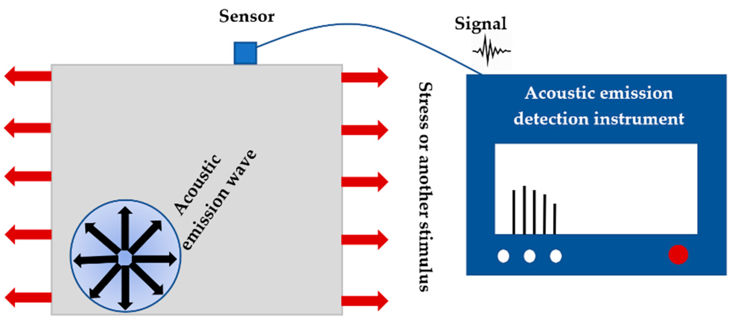
3.1. AE Monitoring of Reinforced Concrete (RC) Structures

A common way to monitor AE is observing the structural degradation. If a crack takes place, a stress wave is generated, and it is regarded as an AE source. Due to the stress wave, the resulting stimulus acts upon the specimen material and creates a local plastic deformation [35]. After that, the stress wave flows starting from the source to the surface of the structure and is recorded by an AE sensor. The role of sensors is important for an AE system, since it converts the stress wave to an electrical signal [35]. Signal amplification is necessary prior to transmission given the fact that the sensor is nonintegral. Integral sensors have embedded amplifiers. The wave is directly transferred to the AE instrument for these sensors. Next, the wave is transmitted for data acquisition in order to perform recording, storing, and analysis. A basic pictorial view of the AE data acquisition for a reinforced concrete beam is presented in Figure 1.
It is quite challenging to perform AE monitoring for composite materials like RC beams because of the attenuation effect. RC beams are heterogeneous materials consisting of cement, coarse aggregates, fine aggregates, and steel bars as reinforcement. Additionally, it is full of flows like pores, air voids, etc. Therefore, a suitable sensor with a lower resonant frequency and appropriate frequency range should be chosen.

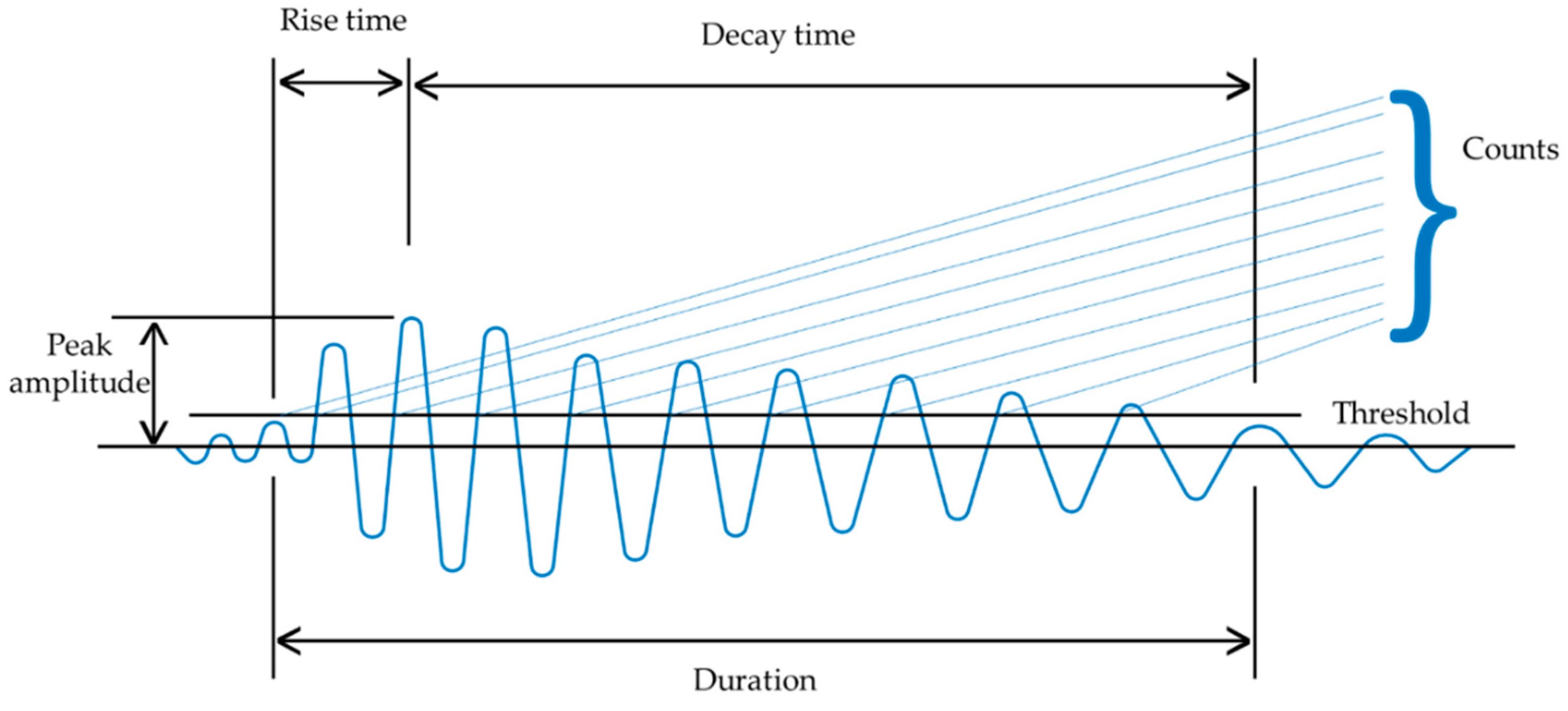
3.2. Acoustic Emission Burst Features

AE signals collected from the concrete structures have special parameters that can represent AE events in a descriptive way. These AE features characterize the AE bursts that are considered to develop the crack assessment and classification methods in this study. The AE features we used in our study are the peak amplitude, AE counts, AE energy, rise time, and decay time. Altogether, these combined features will be addressed as AEB features in our study. They are highly related to concrete structural health monitoring, and they are also crucial measures for crack characterization. Figure 2 presents a pictorial view of the features. They are further defined as follows [35,36]:
Peak amplitude: The highest voltage measured in an AE waveform is denoted the peak amplitude.
AE counts: The number of times the AE signal exceeds a preset threshold during any selected portion of the test is defined as the AE counts.
AE energy: Measurement of area conducted within the rectified signal envelope can be defined as AE energy.
Rise time and Decay time: The time between the first threshold crossing and peak amplitude is called the rise time. The decay time is the opposite of the rise time. The time when the peak value of the amplitude reduces to the lowest within the threshold is set prior.

3.3. Boruta-Mahalanobis System

The MD itself can build a noisy time history trend for the occurrence of concrete cracks, but it is not possible to assure features being used by the classifier if all of them are useful. Using features that do not have much impact on finding the proper time history trend of crack occurrence can not only increase the computational complexity but can also introduce a fallacious trend, resulting in unintended and untimely alarms. Therefore, we need a feature selection algorithm to serve our purpose [37]. We incorporated the Boruta feature selector algorithm to sort out the useful features for calculating MDs.
The Boruta algorithm is a wrapper-based feature selection algorithm built using the random forest classification algorithm [38]. It has been successfully used in different fields of fault diagnosis [39,40]. It collects outputs from an ensemble of randomized samples through which it is possible to reduce the misleading effects of random fluctuations and correlations. The extra randomness added by Boruta can present us with a transparent view of the attributes that are crucial for describing the system. The Boruta algorithm is described as follows:
  • First, we have to expand our information system by adding copies of all the variables. The system must be expanded by at least five shadow attributes.
  • It is next required to shuffle the attributes that are newly added to get rid of their correlations with the response.
  • The random forest classifier is invoked at this step on the expanded information system. The Z scores are computed and stored.
  • From the shadow attributes, we must find out the maximum Z score. This score is referred to as MZSA. If any attribute scores better than the MZSA, we are supposed to assign a hit for that.
  • If there is any attribute with an undetermined importance, we have to perform a two-tailed test of equality with the MZSA.
  • There will be attributes in the system that have a significantly lower importance than MZSA. Those attributes are regarded as unimportant and must be wiped out from the information system. We must deem attributes as “important” if they have an importance significantly higher than the MZSA.
  • Finally, we must remove all the shadow attributes and repeat the whole process unless the importance is assigned for all the attributes or the algorithm reaches a prior limit of the number of random forest runs.
After the important features are listed using Boruta, we would use them to find our CAI using the MD. To do that, we have to define the features that represent the normal condition first from the ones selected using Boruta. The data associated with the features that present the normal scenario are next gathered to calculate the MDs of the normal observations. The constructed feature set can be defined as:
F m × n = [ f u v ] m × n
where f u v is the uth observation of the vth reference, m denotes the total number of observations, and n presents the total number of features. It is required for all the variables in the system to contribute equally in order to determine the MD by definition. For this reason, we have to normalize the observations in F. F is normalized as follows:
N u v = ( f u v f ¯ v ) / σ v
where the normalized test feature is represented by N u v . σ is the standard deviation. f ¯ v and σ can be calculated as:
f ¯ v = 1 a u = 1 a f u v
σ = u = 1 a ( f u v f ¯ v ) 2 / ( a 1 )
where a represents the observations in the dataset that are considered healthy. Finally, the MD is calculated using Equation (5), considering the normalization we obtained using Equation (3).
M D   ( u ) = 1 q N u v C 1 N u v T
where C denotes the correlation matrix of the features that are normalized.

3.4. The CUMSUM Algorithm

The CUMSUM is a technique for sequential analysis developed by E. S. Paige [41] that is usually used for change detection for monitoring purposes. In this technique, the quality number θ is used as a parameter of the probability distribution. For example, θ can be the data mean. The CUMSUM method can be devised to deduce changes in the parameter. Additionally, a criterion to decide when to take corrective action is also proposed in the CUMSUM. If we use the CUMSUM algorithm to track changes in θ , it is possible to detect the steps of a time series.
Let the M D [ w ] be a discrete random signal with independent and identically distributed samples that follow a probability density function (PDF). The deterministic parameter can either be a mean ( µ w ) or variance ( σ w 2 ) of the M D [ w ] . The M D [ w ] may contain an abrupt change occurring at the change time w c . Based on the theory proposed by Paige, this change is modeled by the instant modification of θ , taking place at the change time w c . Therefore, θ = θ 0 before w c and θ = θ 1 from w c to the current sample. For the above-mentioned assumptions, the entire PDF of the signal P w , observed between the first sample ( M D   [ 0 ] ) and the current one ( M D   [ k ] ) , can have two different forms:
(a)
Under the no-change hypothesis (H0), the PDF of MD (w) is
P w | H 0 = w = 0 k P   ( M D [ w ] , θ 0 )
(b)
Under one change hypothesis (H1), the PDF is as follows:
P w | H 1 = w = 0 w c 1 P   ( M D [ w ] , θ 0 )   w = w c k P   ( M D [ w ] , θ 1 )
To design the CUMSUM algorithm, a sudden change in the past signal has to be sequentially detected sample after sample. For every new sample M D   [ k ] either H 0 or H 1 must be decided. If H 1 is decided, it is necessary to decide the change time using an estimator, w c ^ . It is quite difficult to choose between H 0 and H 1 . If H 1 is decided, it can be concluded that an abrupt change is detected. One easy way to solve this is calculating the loglikelihood ratio. If the loglikelihood ratio is greater than the set threshold (h), we can determine the set hypothesis to be H 1 . To obtain a simplified version of the algorithm, we need an instantaneous loglikelihood ratio at time w . This is derived by the following equation:
s [ w ] = ln { P ( M D [ w ] , θ 1 ) P ( M D [ w ] , θ 0 ) }
The cumulative sum from 0 to k can be written as
S [ k ] = w = 0 k s [ w ]
The loglikelihood function can be rewritten as
L M D [ k , w c ] = S [ k ] S [ w c 1 ]
Finally, the decision function and the estimator can be written as
G M D [ k ] = S [ k ] min 1 w c k S [ w c 1 ]
w c ^ = arg min 1 w c k S [ w c 1 ]
Algorithm 1 describes the CUMSUM algorithm in brief based on the above discussion and formulations.
Algorithm 1 CUMSUM Algorithm
Initialization
 set the detection threshold h > 0
k = 0
end
whilethe algorithm is not stoppeddo
 measure the current sample MD [k]
s [ k ] = ln { P ( M D [ k ] , θ 1 ) P ( M D [ k ] , θ 0 ) }
S [ k ] = w = 0 k s [ w ]
G M D [ k ] = S [ k ] min 1 w c k S [ w c 1 ]
  if G M D [ k ] > h then
    w d k
    w c ^ = arg min 1 w c k S [ w c 1 ]
   stop or reset the algorithm
  end
   k = k + 1
End

3.5. k-Nearest Neighbor Algorithm

The k-NN [42] algorithm has acceptable performance for data with a small number of features, particularly if there are not many distinguishable outliers. The algorithm works based on three basic principles: (1) the calculation of distances among the neighbors, (2) the determination of the k-closest neighbors to handle the bias invariance trade-off for finding a solution to the overfitting/underfitting phenomena, and (3) votes for labeling the data. Using Figure 3, the basic mechanism of k-NN can easily be explained.
As we can see in Figure 3, the green circle with the question mark is a new sample in the system that we are attempting to classify. It can be classified into either class 01, which is represented by the red polygon, or it may fall under class 02, which is denoted by the purple diamond. When k = 2, we can see that the new data point falls under class 02 because of its high density within the circle. If the value of the k is randomly decided as 3, the new data point falls under class 01, because there are three instances in that class and only two instances from class 02. Selecting an appropriate k value is therefore crucial. If we have a k-value, we can draw boundaries for each class. Another significant parameter alongside the k-value is the distance parameter. Usually, it is calculated as a Euclidian distance using the following equation for any two different points x and y:
D x , y = i = 1 n ( x i y i ) 2

4. Methodology

The methodology proposed in this work is divided into two sections. First, the AE data acquisition process for the RC beam (24 MPa, Korean Standard Reinforced Steel Bar, D16 (SD400)) is conducted. To do this, an experimental setup was built for conducting a three-point bending test on the RC beams with a loading machine to apply an external load. The second portion of the proposed methodology consists of developing a robust CAI by using the AEB features and BMS. Additionally, three-class classification was conducted to differentiate among the normal condition, micro-cracks, and fractures. The second portion ends with an algorithmic representation of the whole crack characterization method (CAI and classification).

4.1. Experimental Test Setup and Data Acquisition

We developed the testbed at our Ulsan industrial artificial intelligence laboratory (UIAI) located in Ulsan, Republic of Korea to acquire the AE data. Flexural tests are popular for evaluating the tensile strength of RC beams. Further, flexural tests can be used to determine the ability of the RC beams to endure failure resulting because of the bending. These tests are performed using center-point bending, three-point bending, or four-point bending. The three-point bending test is carried out in a way where half of the total load is projected at every one-third of the RC beam length. On the other hand, the full load is applied at the center of the beam in center-point bending. Based on the standard set by the American society for testing and materials (ASTM), the length of the RC beam has to be at least three times greater than the depth [43]. The depth of the RC beam we considered was 300 mm. The span length fixed for the experiment was 2400 mm. Since the length was quite large, a three-point bending test was conducted for a uniform distribution of the cracks in the beam.
Figure 4 and Figure 5 present the testbed for gathering AE signals from the test specimen. A diagram showing where the sensors were placed in the RC beam and the conducted three-point bending test is presented in Figure 4. Figure 5 displays the real-time setup developed at the UIAI laboratory. The length of the beam was 2400 mm, and the depth was 300 mm. For a particular amount of time, an external load was applied to initiate the cracks. The loads were projected at two points on the beam that were 800 mm apart from each other. We used a load velocity of 2 mm/s.
Various types of sensors were used for acquiring the AE data. R15I [44] and WD [45] sensors were used in the experimental setup. For every type of sensor, the flexural test was conducted three times, resulting in six different bending tests. The experiments were conducted in the same condition for the reproducibility test. To choose a highly sensitive sensor, a verification of the sensor mounting was undertaken. We used the pencil lead fracture (PLF) test to mimic the acoustic wave on the surface of the concrete structure. For this purpose, a magnetic pencil with a Teflon shoe was used. Readers can refer to [46] for the details of the process. Figure 6 depicts the method to handle the magnetic pencil on the specimen surface. An angle of 300 from the plane of the specimen surface was used (illustrated in Figure 6). If the PLF produces a high amplitude of 99 dB or sensitivity within a ±3-dB margin, we can consider the sensors to be significantly coupled. Through this process, we chose our sensor to be R15I. A total of eight sensors were placed on the concrete beam for data acquisition in each experiment.
The RC beam had six surfaces, and our goal was to cover all of the surfaces using a total of eight sensors. We fixed the sensors on the concrete specimen using mounting tape and glue gel. We put the sensors as far as possible from the loading points, mostly near the ends of the beam, so that the crack formation did not harm the placement of the sensors. AE signals were collected for around 15 min at a 10-MHz sampling rate. The R15I sensors had an integrated amplifier and a preamplifier having a gain of 40 dB. There was no AE threshold set prior to performing the experiments, but an adaptive threshold level was used. The adaptive threshold was dependent on the maximum amplitude of the collected AE signals.
Figure 7 presents the AE signals for three different scenarios. The first one, Figure 7a, represents the normal condition in the beam. Figure 7b,c represents the AE signals for micro-cracks and macro-cracks. Macro-cracks are often referred to as fractures in our study. The in-plane distance was measured using a linear variable differential transformer (LVDT) at the mid-span, which was fixed at the bottom of the concrete specimen. Figure 8 presents the concrete specimen with severe fractures that occurred after the gradual application of the increasing load. Table 1 summarizes the experimental specifications.

4.2. Proposed Methodology for CAI Development and Crack Classification

The proposed methodology of this study consists of CAI development and crack-type classification. The steps of the proposed methodology can be described as follows:
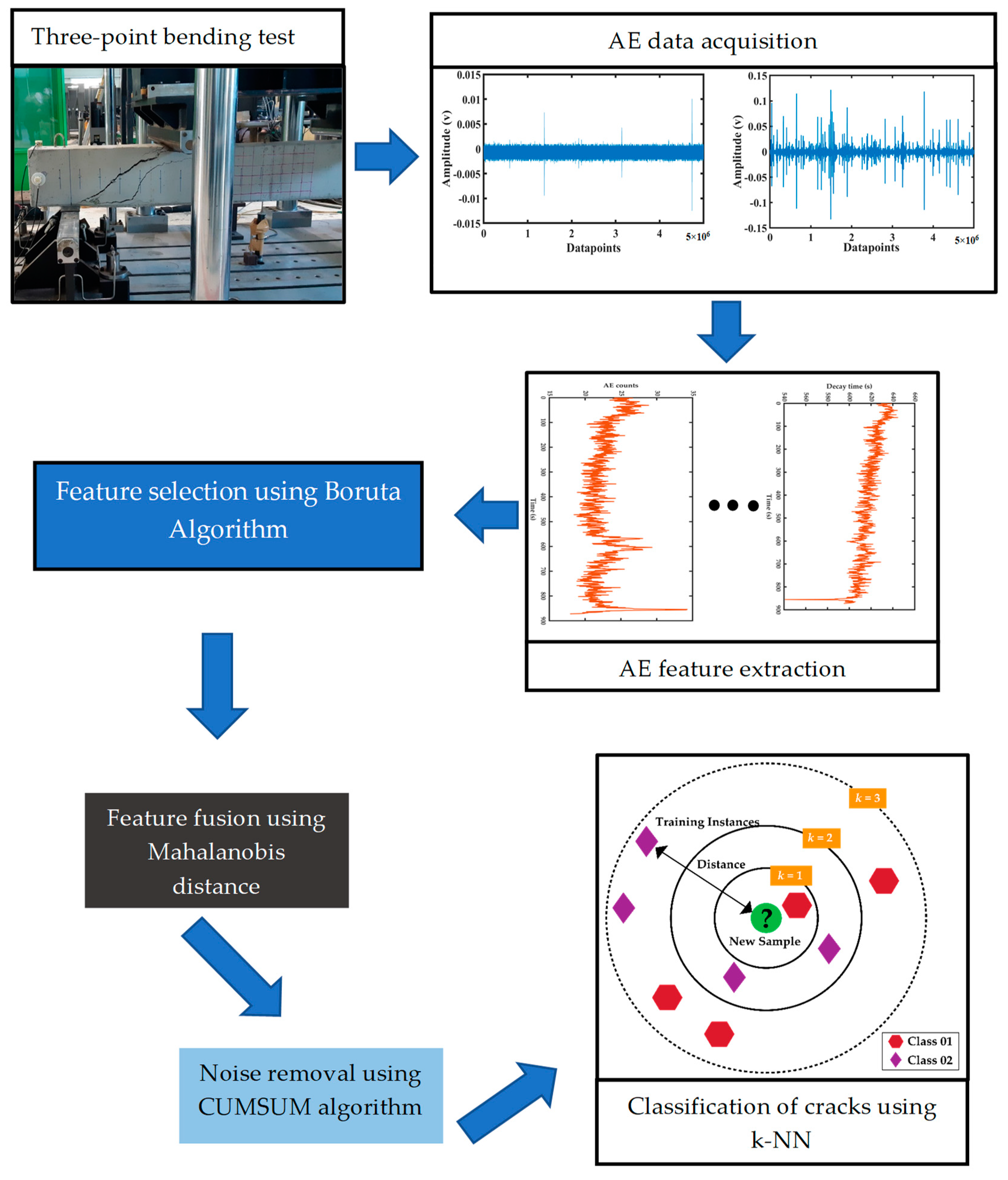
  • AE signals are collected from the testbed that involves conducting three-point bending tests on RC beams.
  • Some AEB features were described in Section 3.1. They are extracted from the collected raw signals.
  • Features representing the condition of the RC beams when there are no cracks are defined first. Next, we collect data of all the features denoting this normal condition. After that, the MDs of the normal condition are calculated.
  • The MDs of the abnormal groups: micro-cracks and macro cracks/fractures are calculated at this step using the MS. These two groups consist of feature points related to micro-crack and macro-crack/fracture formation in the RC beam. To normalize the features of these two abnormal groups, the standard deviation and mean of the corresponding features from the normal group are used. Lastly, the correlation matrix associated with the normal group is adopted to find out the MDs of the two conditions that are abnormal, corresponding to the micro and macro-cracks, respectively.
  • As stated in Section 3.3, the Boruta feature selection algorithm is used in this step to sustain the crucial features.
  • The MD corresponding to the CAI that fuses the crucial features selected using the Boruta algorithm is denoised using Algorithm 1, presented in Section 3.4. Algorithm 1 works perfectly as a NRS and provides us with a monotonic CAI curve.
  • The CAI consists of 872 data points. The first 300 points represent the normal condition with no crack formation in the concrete beam. The next 300 and 272 points represent the micro-cracks and macro-cracks/fractures, respectively. This CAI plot was fed to a k-NN classifier as an input for classification.
Figure 9 presents the comprehensive pictorial view of the proposed method.
To further make our proposed method understandable and implementable for readers, we summarized the entire methodology into an algorithm. The algorithmic view covers all the processes presented in Figure 9. For the technical details of the algorithm, refer to Section 3. Algorithm 2 is described as follows:
Algorithm 2 Algorithm of the proposed method
Step 1: Feature extraction
Step 2: Feature selection using Boruta
Input: Given an information set: I; I N
Output: Relevant features: F; F M ; M N
Initialization
 Shadow information set, S = { S 1 , S k }
s I , s N
H = H i t   a r r a y
end
for ( I , S ) , I p = S k q ; where, p , q = 0 : n ; p q
 Global system, g = { I , S } ;   g   N }
while R a n d l i m i t < the prior limit of the random forest runs, do
   Z s c o r e r a n d o m f o r e s t   ( g )
   important _ feature Z s c o r e I > Z s c o r e s k . max ( )
   omitted _ feature Z s c o r e I < Z s c o r e s k . max ( )
  For two-tailed test of equality, F e q { Z s c o r e I = Z s c o r e s k . max ( ) Z s c o r e I Z s c o r e s k . max ( )
   H i t s , H { 1 ;   Z s c o r e I = Z s c o r e s k . max ( ) 0 ; Z s c o r e I Z s c o r e s k . max ( )
  update H and R a n d l i m i t
end
return F
end
Step 2: MD calculation
Input: Feature set F, F m × n ; a = number of healthy observations
Output: MD of all the features
while calculation of MD is underway, do
F N f ( x ) = { 1 ,     n o r m a l   c o n d i t i o n 0 , o t h e r w i s w
f u v = uth observation of the vth reference, g = Total observations, h = total features
F g × h = [ f u v ]
for 1: (g × h)
  calculate the mean, variance, and normalized feature using equations 3, 4, and 2
calculate the covariance matrix, C for the normalized features
  update F g × h with normalized features
  calculate the MD using Equation (5)
  compute until u
end
return MD
Step 3: Algorithm 1 for noise removal from the MD
Step 4: Classification using the k-NN algorithm

5. Results Analysis

We used MATLAB software and Python 3.5 for the analysis. This section mainly evaluates the potential of the method described in Section 4.2 for the CAI development and classification. First, an analysis of the results is performed to develop a lean and robust CAI in the following section. The section after that contains an analysis of the classification results.

5.1. Feature Extraction and CAI Development

To build our desired CAI for the RC beam, we used five different features (peak amplitude, rise time, decay time, AE counts, and AE energy). There was a total of 872 points for each feature, representing a time history of 872 s during the bending test. Each feature is expected to have a very significant impact on the CAI. Therefore, features that are not correlated with cracks can make the CAI unreliable. Figure 10 shows an example of a reliable and an unreliable feature. Figure 10a shows the trend of the decay time over the entire failure history of the concrete specimen. The value of the decay time changes over time, and it drastically falls at 855 s, representing the failure of the beam. This trend can be used to represent the failure history of the beam. On the other hand, the time history plot of the feature and peak amplitude do not provide us with much insight about the initial crack occurrence and crack expansion and occurrences. Even though the 300–600 s represent the formation of the micro-cracks, the trend in Figure 10b does not provide us with significant fluctuations in that early time period. The peak amplitude feature is therefore not beneficial for our CAI. To solve this issue, we used the Boruta algorithm described in Section 3.3. Figure 11 shows the resulting ranking of the features considered in our study. The three features having the most importance are selected to be fused using the MD combining together all the fault information from each.
A plot of the BMS (selected features and MD) for the concrete’s minor crack formation to fail is presented in Figure 12a. It puts together the degradation information from each of the AE features selected using the Boruta algorithm and comprehensively reflects the crack formation in the beam. Figure 12a shows a clearer crack formation trend compared to any individual feature, since it has less noise. However, the BMS plot still contains noise due to minor oscillations before it starts to fully grow. This can create unwanted maintenance alarms. To achieve our final CAI, the BMS plot is further processed using NRS (the CUMSUM algorithm). Figure 12b contains no noise, and the time history of the crack formation is clearly visible. For the first 300 s, there was no crack, and thus, it denoted the normal condition of the RC beam. Cracks started forming at around 301 s, and we could see the macro-cracks/fractures occurring from 600 s onward. The RC beam went into complete failure at around 855 s.

5.2. Classification Using k-NN

To classify the damage stages, we used the k-NN algorithm. First, we used the classification model with chosen feature vectors that enable the classifier to distinguish the normal condition, micro-cracks, and macro-cracks/fractures. Figure 13 presents the 3D feature space of the selected features that were used in this study. It is clearly visible that clusters for the normal and crack conditions formed. We initially followed the typical process of training the classifier with the chosen feature space but ended up having a low classification accuracy. However, crack characterization and detection for RC structures is a critical task that should have a margin of error that is as low as possible. Any miscalculation may lead to catastrophic outcomes that can cost valuable human lives. To increase our accuracy, we used the CAI plot obtained using the BMS (Figure 12) that clearly indicated the damage to perform the classification. The CAI curve contains all the fault information from the crucial features and has a nice increasing monotonous curve representing the crack formation and expansion over the time history.
As mentioned in Section 3.5, it is quite important to carefully choose the values of k for the k-NN algorithm. We conducted experiments with eight different values of k (1, 3, 5, 7, 9, 11, 13, and 15). From Figure 14, we can see that for k-values of 5, 3, and 1, the testing accuracy was the highest. The accuracy remained unchanged for these three values. We set the k-value of our classification problem to be 5.
We divided our datasets into two parts. Seventy percent of the data was used for training and the rest for testing. The first dataset consisted of the direct feature values (rise time, decay time, and AE counts), and the second dataset consisted of the points derived from the CAI plot. Figure 15 presents the confusion matrix for the proposed approach (k-NN and CAI plot) and k-NN algorithm learning directly from the feature space (k-NN and selected AE features). It is clearly visible from Figure 15b that the direct k-NN classifier misclassified many normal data points as micro-cracks. Additionally, for the typical approach, many micro-crack specimens were classified as macro-cracks/fractures. However, from Figure 15a, we can comprehend that the CAI-based classifier successfully distinguished between micro and macro-cracks with a very low error margin. We also compared our proposed method with a very recently published paper [34] that used the CFAR algorithm with k-NN. For comparison, we used two parameters: the average classification accuracy and F1-score. The F1-score can be calculated as follows:
F 1 s c o r e = 2 × R e c a l l × P r e c i s i o n R e c a l l + P r e c i s i o n
Table 2 presents the performance comparison for the proposed method, the k-NN algorithm with the direct AE feature vectors, and the work presented in [34]. The proposed method outperforms the other two methods in both of the considered parameters with a good margin.

6. Conclusions

This paper proposes an approach that involves developing a robust CAI accompanied by a crack detection method using the k-nearest neighbor (k-NN) algorithm that can successfully distinguish among the normal condition, micro-cracks, and macro-cracks (fractures) of RC beams. The AEB features and BMS were combined to build a novel CAI for evaluating the crack types of RC beams. To do that, the AE signals were first collected from the testbed where three-point bending tests were conducted on RC beams. Second, the AE features were extracted from the raw AE data. Third, using the Boruta feature selection algorithm, the crucial features were selected to form the feature space. They were provided to the system for the calculation of the MD that differentiates the crack conditions from the normal ones. Lastly, the CUMSUM algorithm was used as a NRS to obtain a solid and monotonic CAI without noise. The proposed CAI can effectively track the crack formation trend in the RC beam over its history. This technique can point out the time when premature micro-cracks occur and, also, the time when these cracks expand and eventually lead to failure. This method is quite industry friendly, as it relies on the healthy data from the normal condition and does not necessitate previous information about the failure data. The final stage of this work is the classification of the crack types using k-NN. The CAI plot was fed to the classifier as the input, and it was possible to successfully separate micro-cracks from the macro ones, which is a difficult task that previous works failed to perform. The proposed method achieved a 99.6% accuracy, which is 17.61% higher than the previous approach.

Author Contributions

Conceptualization, M.A.H., C.H.K., and J.-M.K.; data curation, M.A.H.; formal analysis, M.A.H. and C.H.K.; funding acquisition, J.-M.K.; methodology, M.A.H., C.H.K., and J.-M.K.; software, M.A.H.; supervision, J.-M.K.; validation C.H.K. and J.-M.K.; visualization, M.A.H.; writing—original draft, M.A.H.; and writing—review and editing, J.-M.K. All authors have read and agreed to the published version of the manuscript.

Funding

This research was supported by a grant (2019-MOIS41-002) from the National Demand Customized Life Safety R&D Project funded by the Korean Ministry of Interior and Safety (MOIS).

Conflicts of Interest

The authors declare no conflict of interest.

References

  1. Hou, T.C.; Lynch, J.P. Electrical impedance tomographic methods for sensing strain fields and crack damage in cementitious structures. J. Intell. Mater. Syst. Struct. 2009, 20, 1363–1379. [Google Scholar] [CrossRef] [Green Version]
  2. Li, V.C.; Herbert, E. Robust self-healing concrete for sustainable infrastructure. J. Adv. Concr. Technol. 2012, 10, 207–218. [Google Scholar] [CrossRef] [Green Version]
  3. Aldahdooh, M.; Bunnori, N.M. Crack classification in reinforced concrete beams with varying thicknesses by mean of acoustic emission signal features. Constr. Build. Mater. 2013, 45, 282–288. [Google Scholar] [CrossRef]
  4. Aggelis, D.G.; Soulioti, D.V.; Sapouridis, N.; Barkoula, N.M.; Paipetis, A.S.; Matikas, T.E. Acoustic emission characterization of the fracture process in fibre reinforced concrete. Constr. Build. Mater. 2011, 25, 4126–4131. [Google Scholar] [CrossRef]
  5. Nair, A.; Cai, C.S. Acoustic emission monitoring of bridges: Review and case studies. Eng. Struct. 2010, 32, 1704–1714. [Google Scholar] [CrossRef]
  6. Otsuka, K.; Date, H. Otsuka2000.Pdf. Eng. Fract. Mech. 2000, 65, 1–13. [Google Scholar]
  7. Habib, M.A.; Rai, A.; Kim, J.M. Performance degradation assessment of concrete beams based on acoustic emission burst features and Mahalanobis—Taguchi system. Sensors 2020, 20, 3402. [Google Scholar] [CrossRef]
  8. Yu, X.; Bentahar, M.; Mechri, C.; Montrésor, S. Passive monitoring of nonlinear relaxation of cracked polymer concrete samples using acoustic emission. J. Acoust. Soc. Am. 2019, 146, EL323–EL328. [Google Scholar] [CrossRef] [Green Version]
  9. Das, A.K.; Suthar, D.; Leung, C.K.Y. Machine learning based crack mode classification from unlabeled acoustic emission waveform features. Cem. Concr. Res. 2019, 121, 42–57. [Google Scholar] [CrossRef]
  10. Aggelis, D.G.; De Sutter, S.; Verbruggen, S.; Tsangouri, E.; Tysmans, T. Acoustic emission characterization of damage sources of lightweight hybrid concrete beams. Eng. Fract. Mech. 2019, 210, 181–188. [Google Scholar] [CrossRef]
  11. Aggelis, D.G. Classification of cracking mode in concrete by acoustic emission parameters. Mech. Res. Commun. 2011, 38, 153–157. [Google Scholar] [CrossRef]
  12. Banjara, N.K.; Sasmal, S.; Srinivas, V. Investigations on acoustic emission parameters during damage progression in shear deficient and GFRP strengthened reinforced concrete components. Measurement 2019, 137, 501–514. [Google Scholar] [CrossRef]
  13. Tsangouri, E.; Remy, O.; Boulpaep, F.; Verbruggen, S.; Livitsanos, G.; Aggelis, D.G. Structural health assessment of prefabricated concrete elements using Acoustic Emission: Towards an optimized damage sensing tool. Constr. Build. Mater. 2019, 206, 261–269. [Google Scholar] [CrossRef]
  14. Yue, J.G.; Kunnath, S.K.; Xiao, Y. Uniaxial concrete tension damage evolution using acoustic emission monitoring. Constr. Build. Mater. 2020, 232, 117281. [Google Scholar] [CrossRef]
  15. Chen, C.; Fan, X.; Chen, X. Experimental investigation of concrete fracture behavior with different loading rates based on acoustic emission. Constr. Build. Mater. 2020, 237, 117472. [Google Scholar] [CrossRef]
  16. Pantazopoulou, S.J.; Zanganeh, M. Assessing damage in corroded reinforced concrete using acoustic emission. J. Mater. Civ. Eng. 2001, 13, 340–348. [Google Scholar] [CrossRef]
  17. Carpinteri, A.; Lacidogna, G.; Paggi, M. Acoustic emission monitoring and numerical modeling of FRP delamination in RC beams with non-rectangular cross-section. Mater. Struct. Constr. 2007, 40, 553–566. [Google Scholar] [CrossRef]
  18. Verma, S.K.; Bhadauria, S.S.; Akhtar, S. Review of nondestructive testing methods for condition monitoring of concrete structures. J. Constr. Eng. 2013, 1–11. [Google Scholar] [CrossRef] [Green Version]
  19. Holford, K.M.; Davies, A.W.; Pullin, R.; Carter, D.C. Damage location in steel bridges by acoustic emission. J. Intell. Mater. Syst. Struct. 2001. [Google Scholar] [CrossRef]
  20. ElBatanouny, M.K.; Larosche, A.; Mazzoleni, P.; Ziehl, P.H.; Matta, F.; Zappa, E. Identification of cracking mechanisms in scaled FRP reinforced concrete beams using acoustic emission. Exp. Mech. 2014, 54, 69–82. [Google Scholar] [CrossRef]
  21. Ranjith, P.G.; Jasinge, D.; Song, J.Y.; Choi, S.K. A study of the effect of displacement rate and moisture content on the mechanical properties of concrete: Use of acoustic emission. Mech. Mater. 2008, 40, 453–469. [Google Scholar] [CrossRef]
  22. Ohno, K.; Ohtsu, M. Crack Classification in concrete based on acoustic emission. Constr. Build. Mater. 2010, 24, 2339–2346. [Google Scholar] [CrossRef]
  23. Yun, H.D.; Choi, W.C.; Seo, S.Y. Acoustic emission activities and damage evaluation of reinforced concrete beams strengthened with CFRP sheets. NDT E Int. 2010, 43, 615–628. [Google Scholar] [CrossRef]
  24. Sagar, R.V.; Prasad, B.K.R.; Sharma, R. Evaluation of damage in reinforced concrete bridge beams using acoustic emission technique. Nondestruct. Test. Eval. 2012, 27, 95–108. [Google Scholar] [CrossRef]
  25. Huang, S.F.; Li, M.M.; Xu, D.Y.; Zhou, M.J.; Xie, S.H.; Cheng, X. Investigation on a kind of embedded ae sensor for concrete health monitoring. Res. Nondestruct. Eval. 2013, 24, 202–210. [Google Scholar] [CrossRef]
  26. Mahalanobis, P.C. Reprint of: Mahalanobis, P.C. (1936) “On the generalised distance in statistics.”. Sankhya A 2018, 80, 1–7. [Google Scholar] [CrossRef]
  27. Kursa, M.B.; Jankowski, A.; Rudnicki, W.R. Boruta—A system for feature selection. Fundam. Inform. 2010. [Google Scholar] [CrossRef]
  28. Morales-Esteban, A.; Martínez-Álvarez, F.; Scitovski, S.; Scitovski, R. A fast partitioning algorithm using adaptive Mahalanobis clustering with application to seismic zoning. Comput. Geosci. 2014. [Google Scholar] [CrossRef]
  29. Shang, J.; Chen, M.; Zhang, H. Fault detection based on augmented kernel Mahalanobis distance for nonlinear dynamic processes. Comput. Chem. Eng. 2018. [Google Scholar] [CrossRef]
  30. Ruiz de la Hermosa González-Carrato, R. Wind farm monitoring using Mahalanobis distance and fuzzy clustering. Renew. Energy 2018. [Google Scholar] [CrossRef]
  31. Jin, X.; Ma, E.W.M.; Cheng, L.L.; Pecht, M. Health monitoring of cooling fans based on mahalanobis distance with mRMR feature selection. IEEE Trans. Instrum. Meas. 2012. [Google Scholar] [CrossRef]
  32. Lin, J.; Chen, Q. Fault diagnosis of rolling bearings based on multifractal detrended fluctuation analysis and Mahalanobis distance criterion. Mech. Syst. Signal Process. 2013. [Google Scholar] [CrossRef]
  33. MacGregor, J.F.; Kourti, T. Statistical process control of multivariate processes. Control Eng. Pract. 1995. [Google Scholar] [CrossRef]
  34. Tra, V.; Kim, J.-Y.; Jeong, I.; Kim, J.-M. An acoustic emission technique for crack modes classification in concrete structures. Sustainability 2020, 12, 6724. [Google Scholar] [CrossRef]
  35. Noorsuhada, M.N. An overview on fatigue damage assessment of reinforced concrete structures with the aid of acoustic emission technique. Constr. Build. Mater. 2016, 112, 424–439. [Google Scholar] [CrossRef]
  36. Ali, S.M.; Hui, K.H.; Hee, L.M.; Leong, M.S.; Abdelrhman, A.M.; Al-Obaidi, M.A. Observations of changes in acoustic emission parameters for varying corrosion defect in reciprocating compressor valves. Ain Shams Eng. J. 2019, 10, 253–265. [Google Scholar] [CrossRef]
  37. Hasan, M.J.; Uddin, J.; Pinku, S.N. A Novel Modified SFTA Approach for Feature Extraction. In Proceedings of the 3rd International Conference on Electrical Engineering and Information Communication Technology (ICEEICT), Dhaka, Bangladesh, 22–24 September 2016; pp. 1–5. [Google Scholar]
  38. Breiman, L. Random forests. Mach. Learn. 2001. [Google Scholar] [CrossRef] [Green Version]
  39. Hasan, M.J.; Kim, J.; Kim, C.H.; Kim, J.M. Health state classification of a spherical tank using a hybrid bag of features and K-Nearest neighbor. Appl. Sci. 2020, 10, 2525. [Google Scholar] [CrossRef] [Green Version]
  40. Hasan, M.J.; Kim, J.M. A hybrid feature pool-based emotional stress state detection algorithm using EEG signals. Brain Sci. 2019, 9, 376. [Google Scholar] [CrossRef] [PubMed] [Green Version]
  41. Page, E.S. Cumulative sum charts. Technometrics 1961. [Google Scholar] [CrossRef]
  42. Peterson, L. K-nearest neighbor. Scholarpedia 2009. [Google Scholar] [CrossRef]
  43. ASTM International—Standards Worldwide. Available online: https://www.astm.org/ (accessed on 6 April 2020).
  44. R15I-AST Sensor. Available online: http://www.pacndt.com/downloads/Sensors/IntegralPreamp/R15I-AST.pdf (accessed on 29 May 2020).
  45. WD—100-900 KHZ Wideband Differential AE Sensor. Available online: https://www.physicalacoustics.com/by-product/sensors/WD-100-900-kHz-Wideband-Differential-AE-Sensor (accessed on 29 May 2020).
  46. ASTM. ASTM E976-10, Standard Guide for Determining the Reproducibility of Acoustic Emission Sensor Response; ASTM: West Conshohocken, PA, USA, 2010. [Google Scholar]
Figure 1. Basic acoustic emission (AE) data acquisition system for concrete beams.
Applsci 10 07918 g001
Figure 2. A pictorial representation of the considered AE features.
Applsci 10 07918 g002
Figure 3. A pictorial illustration of the k-nearest neighbor (k-NN) algorithm.
Applsci 10 07918 g003
Figure 4. Schematic diagrams of the testbed: (a) the sensor placement, and (b) the three-point bending test for the beam.
Applsci 10 07918 g004
Figure 5. The real-time experimental testbed for the reinforced concrete (RC) beam: (a) the entire setup and (b) measurement of the cracks.
Applsci 10 07918 g005
Figure 6. The pencil lead fracture test for sensor selection.
Applsci 10 07918 g006
Figure 7. AE signals presenting three different conditions: (a) the normal condition, (b) micro-cracks, and (c) macro-cracks/fractures.
Applsci 10 07918 g007
Figure 8. Macro-cracks/fractures taking place after the application of a gradually increasing load.
Applsci 10 07918 g008
Figure 9. An overview of the proposed method. CUMSUM: cumulative sum.
Applsci 10 07918 g009
Figure 10. Time history of (a) the decay time (a reliable feature) and (b) peak amplitude (an unreliable feature).
Applsci 10 07918 g010
Figure 11. Ranking the features using the Boruta algorithm.
Applsci 10 07918 g011
Figure 12. Time history of the RC beam: (a) Boruta-Mahalanobis system (BMS) plot and (b) final crack assessment indicator (CAI).
Applsci 10 07918 g012
Figure 13. 3D plot of the feature space.
Applsci 10 07918 g013
Figure 14. Determining the optimal value of k.
Applsci 10 07918 g014
Figure 15. Confusion matrix: (a) k-NN and CAI plot and (b) k-NN and selected AE features.
Applsci 10 07918 g015
Table 1. Parameters and specifications of the conducted experiments. RC: reinforced concrete.
SpecificationValue
Number of sensors per experiment 8
Sensor typeWD and R15I AE sensors
Sensor elected after pencil lead fracture testR15I
Number of RC beams6
Data acquisition periodAround 15 min
Concrete type24 MPa
Reinforcement Korean Standard Reinforced Steel Bar, D16 (SD400)
Load1.03 kN (initial) and 107.6 kN (final)
Load velocity2 mm/s
Displacement type In-plane
Displacement measurement locationMid-span
Table 2. Performance comparison of the different approaches. K-NN: k-nearest neighbor, CAI: crack assessment indicator, and AE: acoustic emission.
MethodsAccuracy (%)F1-Score
k-NN and CAI plot99.60.988
k-NN and selected AE features740.738
k-NN and CFAR82.460.819
Publisher’s Note: MDPI stays neutral with regard to jurisdictional claims in published maps and institutional affiliations.

