Adaptive Observer-Based Fault Detection and Fault-Tolerant Control of Quadrotors under Rotor Failure Conditions

Featured Application

This method provides a rotor fault detection and fault tolerance control mechanism for a quadrotor to achieve safety flight even in the presence of single rotor loss.

Abstract

This paper aims to propose a strategy for the flight control of quad-rotors under single rotor failure conditions. The proposed control strategy consists of two stages—fault detection (FD) and fault tolerant control (FTC). A dual observer-based strategy for FD and fault estimation is developed. With the combination of the results from both observers, the decision making in whether a fault actually happened or the observed anomaly was caused by an external disturbance could be distinguished. Following the FD result, a control strategy for normal flight, as well as the abnormal one, is presented. The FTC considers a real-time coordinate transformation scheme to manipulate the target angles for the quad-rotor to follow a prescribed trajectory. When a rotor fault happens, it is going to be detected by the dual observers and then the FTC is activated to stabilize the system such that the trajectory following task can still be fulfilled. Furthermore, in order to achieve robust flight in the presence of external wind perturbation, the sliding mode control (SMC) theory is further integrated. Simulations illustrate the effectiveness and feasibility of the proposed method.

1. Introduction

Quadrotors have been widely used in many fields, such as agriculture, cargo delivery, surveillance, aerial photography, military fields and environmental monitoring [1]. This evidently reveals that the flying area of quadrotors gradually covers most of the areas where people live. Therefore, the safety of people under the flying area is now a concerned and an important issue. To ensure the safety of flight of the quad-rotor and the safety of people under or nearby the flying area, it is necessary to adopt an appropriate field safety strategy, such as fault-tolerant control, when a quad-rotor is malfunctioning.

Actually, FTC strategies have been investigated for decades and applied to many different fields. Among various methods for FTC published in the literature, observer-based approaches are effective and reliable. In [2], a speed sensor FTC for electric-vehicle (EV) powertrains was proposed. The approach considers two observers and a voting algorithm for the sensor fault decision making. Based on a higher order sliding mode (HOSM) observer, a reconfiguration scheme is proposed to maintain a good speed tracking control performance of a permanent-magnet synchronous motor in the event of sensor faults/failures [3]. To achieve on-line speed sensor fault detection, a simple adaptive observer-based scheme for induction motors is developed in [4] for the FTC of EVs under cruise operation mode. However, external vehicular disturbances, which may perturb the fault estimation accuracy, were not considered.

In the literature, many other FTC methods have also been proposed for quadrotor systems, such as model-reference adaptive control [5,6,7], multiple model switching and tuning [8,9,10,11,12,13], feedback linearization [14] and sliding mode control [15,16,17]. Generally, FTC can be classified into passive and active FTC [18,19], which relies on the fault detection and isolation (FDI) result. The techniques of FDI [20] could be classified as model-based [21,22] and data driven [23,24,25] approaches. Model-based methods are more economical and efficient as they do not require one to process massive datasets. An example is demonstrated in [26], which shows that with accurate fault information, the corresponding FTC could be implemented precisely and immediately when faults occur. In some papers, nonlinear adaptive thresholds are designed to enhance the robustness and fault sensitivity of the properties FDI algorithm [27,28]. Moreover, a Thau observer is applied in [29] to generate a diagnostic residue whose value would be almost zero without faults happening inside the fault detection system, but in practical cases, it is hard for the residual to be zero owing to noise, disturbance and the system uncertainties. Hence, an adaptive threshold is adopted to ensure the system robustness and to judge if the real fault exists or not. Another adaptive Thau observer (ATO) was proposed in [30]. Based on the residuals monitoring, the FDI aims to identify the faults as well as estimate the fault offset parameters.

Different from the former study, an innovative fault diagnosis strategy was developed to not only detect the actuators fault, but also to quantify the magnitude of faults. Nevertheless, it would take much time to process the fault estimation since it used some techniques to improve and optimize the original observer, like compensating for the uncertainties based on system identification and filtering the noise by a specified low-pass filter. Some examples of applications of FTC and FDI on aircraft are revealed. For instance, developing a flight control algorithm based on a linear parameter varying (LPV) controller to fulfill tracking during normal and fault conditions [16,31,32]. The study [33] designs adaptive sliding mode Thau observer (ASTMO) to derive the estimation of fault magnitude and the system parameters are solved in terms of the linear matrix inequalities (LMIs). Recently, actuator fault estimation and FTC was demonstrated using model-based observer as well [34]. The study considers a quadrotor vertical take-off and landing scenario subject to partial fault rotor damage. An aggressive fault on a rotor up to 80% is considered. However, a total loss of a rotor was not considered.

Different from the previous studies, in this paper, a dual observer-based strategy for FD and fault estimation is developed. The main objective is to stabilize and control the quadrotor subject to a total loss of a single rotor. Furthermore, with the combination of the residuals from both observers, the decision making process can distinguish whether a fault actually happened or the anomaly was caused by an external disturbance. The proposed FTC of quadrotors further provides a feasible way to deal with potential risks during flight. With model-based FDI scheme, the faults of a quadrotor would be detected by the combination of a nonlinear observer and an adaptive observer, which improves the sensitivity and accuracy of the FD result. Therefore, with the signals generated from the two observers, the real rotor failure can be isolated, so as to activate the FTC laws. Finally, simulations are performed to verify the feasibility of the flight control under a single rotor failure.

2. Dynamic Modeling

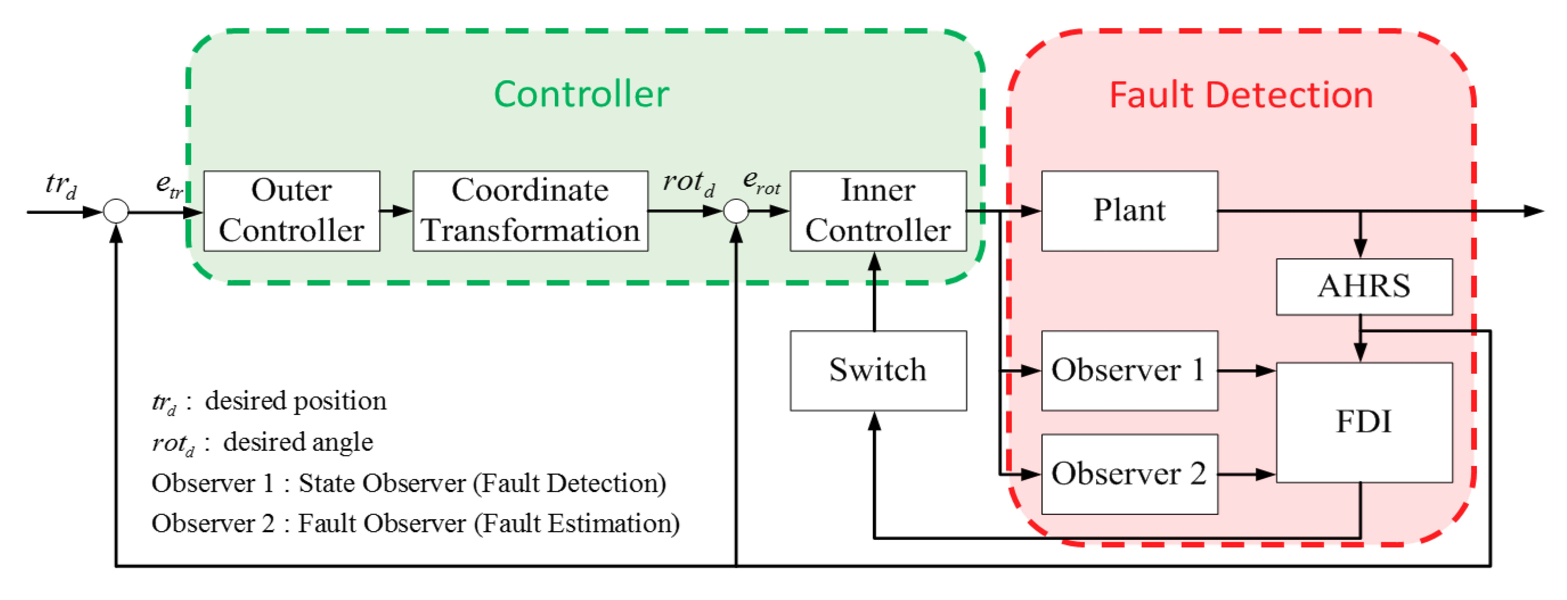
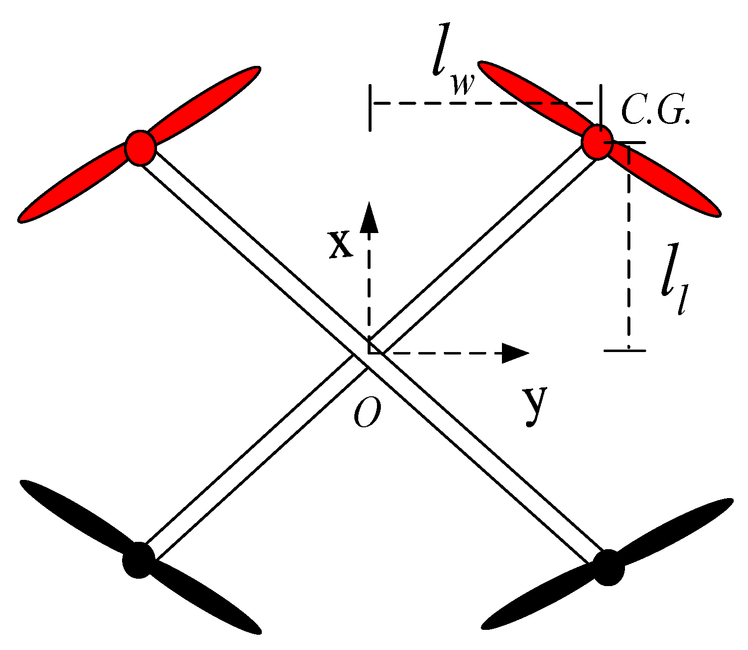
2.1. Configuration of the Quadrotor

The following are the assumptions of the quadrotor to be discussed, including the coordinate definition, variables for geometry configuration, force directions of the thrust, spin directions of propellers, and the heading of the quad-rotor.

In this paper, the coordinate of the vehicle is set to be the Cartesian one with the north-east-down (NED) definition. The cross point of the quadrotor is denoted as C.G. and it is also the origin point of the body-fixed frame. Moreover, the heading of the quad-rotor is along with the x axis as shown in Figure 1. Notice that the propellers’ colors carry different meaning—the red propellers are set to be the same side of the heading as the black ones are on the tail side of the quad-rotor. We assume that the quad-rotor is symmetric about the cross section and the distance between propeller and the origin point of body-fixed frame are l_l and l_w shown in Figure 1. The thrust of propellers are pointing upward, expressed as f_i, and the angular velocity of each propeller is defined as ω_pi shown in Figure 2, where i denotes the i_th propeller.

2.2. Governing Equations

The force equation, including disturbance caused by drag force and wind force, in the x, y, and z direction of the earth frame is formed as below:

$$m{\left[\begin{array}{c}\ddot{x}\\ \ddot{y}\\ \ddot{z}\end{array}\right]}_E={}^{E}R^B{\left[\begin{array}{c}0\\ 0\\ u\end{array}\right]}_B-{\left[\begin{array}{c}{\delta }_x\dot{x}\\ {\delta }_y\dot{y}\\ {\delta }_z\dot{z}\end{array}\right]}_E+{\left[\begin{array}{c}{f}_{wx}\\ f_{wy}\\ f_{wz}\end{array}\right]}_E+{\left[\begin{array}{c}0\\ 0\\ mg\end{array}\right]}_E$$

(1)

where δ_x, δ_y and δ_z denote the drag coefficients; f_wx, f_wy and f_wz denote disturbances caused by wind. u is the composition of forces of the four propellers; that is $u=-f_1-f_2-f_3-f_4$.

^ER^B is the body 3-2-1 rotation transformation matrix that transfers vectors expressed in body-fixed frame to the one expressed in the earth frame. The definition of ^ER^B is as follows:

$${}^{E}R^B=\left[\begin{array}{ccc}\cos \psi & -\sin \psi & 0\\ \sin \psi & \cos \psi & 0\\ 0& 0& 1\end{array}\right]\left[\begin{array}{ccc}\cos \theta & 0& \sin \theta \\ 0& 1& 0\\ -\sin \theta & 0& \cos \theta \end{array}\right]\left[\begin{array}{ccc}1& 0& 0\\ 0& \cos \varphi & -\sin \varphi \\ 0& \sin \varphi & \cos \varphi \end{array}\right]$$

With the rotation transformation matrix, the control input, u, which is acting in the z direction of the body-fixed frame of the quad-rotor, could be transformed into the vector expressed in the earth frame. Therefore, Equation (1) could be written the vector form as indicated below:

$$a_B=\frac{1}{m}{F}_E+g+f_t$$

(2)

where $F_E={}^{E}R^B{\left[\begin{array}{ccc}0& 0& u\end{array}\right]}^T$, $g={\left[\begin{array}{ccc}0& 0& g\end{array}\right]}^T$, $f_t=D_t+d_t$, $D_t=-{\left[\begin{array}{ccc}{\delta }_x\dot{x}& {\delta }_y\dot{y}& {\delta }_z\dot{z}\end{array}\right]}^{\mathrm{T}}$ and $d_t={\left[\begin{array}{ccc}{f}_{wx}& f_{wy}& f_{wz}\end{array}\right]}^T$.

In moment equation, the derivative of angular velocity of the quadrotor is defined as ${\dot{\mathsf{\omega }}}_B\in {\mathbb{R}}^{3\times 1}$, the moment of inertia of the quadrotor is defined as J $\in {\mathbb{R}}^{3\times 3}$, the torque generated from the propellers is defined as τ_η $\in {\mathbb{R}}^{3\times 1}$, the wind disturbance is defined as d_η $\in {\mathbb{R}}^{3\times 1}$, the gyroscope effects and the rest terms is defined as P.

The governing equations are summarized below:

$${\dot{\mathsf{\omega }}}_B=J^{-1}\left({\mathsf{\tau }}_{\eta }-P+f_{\eta }\right)$$

(3)

where:

$$\{\begin{array}{l}P={\mathsf{\omega }}_B\times I_B{\mathsf{\omega }}_B+r_{ct}\times m_p{a}_o\\ +{\displaystyle \sum _{i=1}^4\left[r_{ci}\times m_p\left({\mathsf{\omega }}_B\times \left({\mathsf{\omega }}_B\times r_{ci}\right)\right)+{\mathsf{\omega }}_B\times I_p\left({\mathsf{\omega }}_B+{\mathsf{\omega }}_{pi}\right)\right]}\\ {\mathsf{\tau }}_{\eta }=\left[\begin{array}{c}\left(f_2+f_3-f_1-f_4\right)l_w\\ \left(f_1+f_2-f_3-f_4\right)l_l\\ \left(f_2-f_1+f_4-f_3\right)\mu \end{array}\right], r_{ct}={\displaystyle \sum _{i=1}^4{r}_{ci}}, f_{\eta }=D_{\eta }+d_{\eta }\\ D_{\eta }=-{\left[\begin{array}{ccc}{\delta }_x\dot{\varphi }& {\delta }_y\dot{\theta }& {\delta }_z\dot{\psi }\end{array}\right]}^T, d_{\eta }={\left[\begin{array}{ccc}{f}_{w\varphi }& f_{w\theta }& f_{w\psi }\end{array}\right]}^T\end{array}$$

(4)

In (3), μ denotes the lift to torque coefficient, I_B denotes the moment of inertia of the quadrotor without rotors, a_o denotes the acceleration of the quadrotor, r_ci denotes the vector pointing from O to the C.G. of i_th propeller, I_p denotes the moment of inertia of the propeller, ω_pi denotes the angular velocity of i_th propeller.

In this paper, the propellers’ dynamics are also taken into consideration, which makes the equation derivation complicated, although these additional terms may be negligible since many papers do not include the effect of the propellers and some of the terms relative to the propellers are relatively small comparing to the quad-rotor. Nevertheless, in this work, we are trying to model for the quadrotor in detail and observe the terms that would affect the rotational motion of the drone. Moreover, for flight properties analysis considering different rotor space configurations readers can refer to [35].

Equation (3) represents the body frame rotational dynamics, which means one could get the angular velocity at different instants. From the control point of view, the global orientation of the drone should be calculated. The relationship between the variation of the Euler angle and the body frame angular velocity is described by [36]:

$$\underset{\dot{\mathsf{\eta }}}{\underbrace{\left[\begin{array}{c}\dot{\varphi }\\ \dot{\theta }\\ \dot{\psi }\end{array}\right]}}=\underset{H}{\underbrace{\left[\begin{array}{ccc}1& \sin \varphi \tan \theta & \cos \varphi \tan \theta \\ 0& \cos \varphi & -\sin \varphi \\ 0& \sin \varphi \sec \theta & \cos \varphi \sec \theta \end{array}\right]}}\underset{{\mathsf{\omega }}_B}{\underbrace{\left[\begin{array}{c}{\omega }_{Bx}\\ {\omega }_{By}\\ {\omega }_{Bz}\end{array}\right]}}$$

(5)

Differentiating Equation (5) gives:

$$\ddot{\mathsf{\eta }}=\dot{H}{\mathsf{\omega }}_B+H{\dot{\mathsf{\omega }}}_B$$

(6)

Substituting Equation (3) into Equation (6) gives the complete dynamics for quadrotor represented as follows:

$$\ddot{\mathsf{\eta }}=\dot{H}{H}^{-1}\dot{\mathsf{\eta }}+H{J}^{-1}\left({\mathsf{\tau }}_{\eta }-P+f_{\eta }\right)$$

(7)

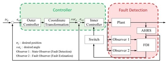
3. Coordinate Transformation-Based Fault-Tolerant Control

3.1. Controller Design

During the loss of a single rotor, the applied torque can no longer achieve ordinary orientation control. This specific scenario could be regarded as a reduced attitude stabilization problem [37]. In order to maintain flight stability under rotor failure conditions, the control effort on yaw dynamics should be determined [38]. Meanwhile, since there is no control effort imposed on the yaw dynamics, there would be an unexpected yaw motion such that incorrect control torque vector may be induced. Thus, the flight controller in this paper consists of two parts—a coordinate transformation based outer-loop controller and an inner-loop stabilization controller illustrated in Figure 3.

From Equation (1), it can be represented in detail by:

$$\ddot{x}=\sin \theta \cos \varphi \frac{u}{m}+\frac{1}{m}\left(f_{wx}-\delta \dot{x}\right)$$

(8)

$$\ddot{y}=-\sin \varphi \frac{u}{m}+\frac{1}{m}\left(f_{wy}-\delta \dot{y}\right)$$

(9)

$$\ddot{z}=\cos \theta \cos \varphi \frac{u}{m}+\frac{1}{m}\left(f_{wz}-{\delta }_z\dot{z}+mg\right)$$

(10)

For translational dynamics Equations (8)–(10), the sliding mode variables for x, y and z are defined respectively as follows:

$$s_x={\dot{e}}_x+{\lambda }_x{e}_x$$

(11)

$$s_y={\dot{e}}_y+{\lambda }_y{e}_y$$

(12)

$$s_z={\dot{e}}_z+{\lambda }_z{e}_z$$

(13)

By taking the derivative of Equations (11)–(13), the control law could be obtained:

$$\begin{array}{l}{u}_x=u_{xeq}+u_{xn}\\ u_y=u_{yeq}+u_{yn}\\ u_z=u=u_{zeq}+u_{zn}\end{array}$$

(14)

where:

$$\begin{array}{l}{u}_{xeq}=m\left({\ddot{x}}_d-{\lambda }_x\left(\dot{x}-{\dot{x}}_d\right)\right)/\left(u\cos \theta \cos \varphi \right)\\ u_{yeq}=m\left({\ddot{y}}_d-{\lambda }_y\left(\dot{y}-{\dot{y}}_d\right)\right)=\left(u\cos \varphi \right)\\ u_{zeq}=m\left(-g+{\ddot{z}}_d-{\lambda }_z\left(\dot{z}-{\dot{z}}_d\right)\right)/\left(\cos \theta \cos \varphi \right)\end{array}$$

(15)

and:

$$\begin{array}{l}{u}_{xn}=-{\rho }_x\frac{m}{u\cos \theta \cos \varphi }\left(\frac{s_x}{\left|s_x\right|+{\epsilon }_x}\right)\\ u_{yn}=-{\rho }_y\frac{m}{\cos \theta \cos \varphi u}\left(\frac{s_y}{\left|s_y\right|+{\epsilon }_y}\right)\\ u_{zn}=-{\rho }_z\frac{m}{\cos \theta \cos \varphi }\left(\frac{s_z}{\left|s_z\right|+{\epsilon }_z}\right)\end{array}$$

(16)

The parameters ρ_x, ρ_y and ρ_z are applied switching gains, and ε_x, ε_y and ε_z are the scaling parameters of the sigmoid function, which are used to eliminate the chattering problem of SMC.

To achieve trajectory tracking control in the presence of heading variation, the virtual control inputs are applied to the x and y:

$${\theta }_d={\tan }^{-1}\left(u_x\right)$$

(17)

$${\varphi }_d={\tan }^{-1}\left(u_y\right)$$

(18)

Equations (17) and (18) are described in an Earth frame, and are used to generate corrected roll and pitch commands when the heading is varying. In other words, the yaw angle obtained from measurement should be applied as a coordinate transformation to get the desired angles such that the torque can be correctly distributed even in the presence of unexpected yaw rotations.

With the aid of the yaw-angle based coordinate transformation, the desired angles could be expressed in the body-fixed frame by:

$${\left[\begin{array}{c}{\varphi }_d\\ {\theta }_d\\ {\psi }_d\end{array}\right]}_B=\left[\begin{array}{ccc}\cos \psi & \sin \psi & 0\\ -\sin \psi & \cos \psi & 0\\ 0& 0& 1\end{array}\right]{\left[\begin{array}{c}{\varphi }_d\\ {\theta }_d\\ {\psi }_d\end{array}\right]}_E$$

(19)

where B denotes body-fixed frame and E denotes the Earth frame.

The desired angles could be obtained by Equations (17)–(19). Combining with Equation (7), the sliding variables are defined as the vector form:

$${\mathbf{s}}_{\eta }={\dot{\mathbf{e}}}_{\eta }+\mathsf{\lambda }{\mathbf{e}}_{\eta }$$

(20)

Design the sliding control torque as follows:

$${\mathsf{\tau }}_{\eta }={\mathsf{\tau }}_{\eta eq}+{\mathsf{\tau }}_{\eta n}$$

(21)

where:

$$\begin{array}{l}{\mathsf{\tau }}_{\eta eq}=\mathbf{J}{\mathbf{H}}^{-1}\left(-\dot{\mathbf{H}}{\mathbf{H}}^{-1}\dot{\mathsf{\eta }}+\mathbf{H}{\mathbf{J}}^{-1}\mathbf{P}+{\ddot{\mathsf{\eta }}}_d-\lambda \left(\dot{\mathsf{\eta }}-{\dot{\mathsf{\eta }}}_d\right)\right)\\ {\mathsf{\tau }}_{\eta n}=-\mathbf{J}{\mathbf{H}}^{-1}{\mathsf{\varrho }}_{\eta }\frac{{\mathbf{s}}_{\eta }}{\Vert {\mathbf{s}}_{\eta }\Vert +\Vert {\mathsf{\epsilon }}_{\eta }\Vert }\end{array}$$

(22)

Following is the proof of the closed-loop stability.

3.2. Stability Analysis

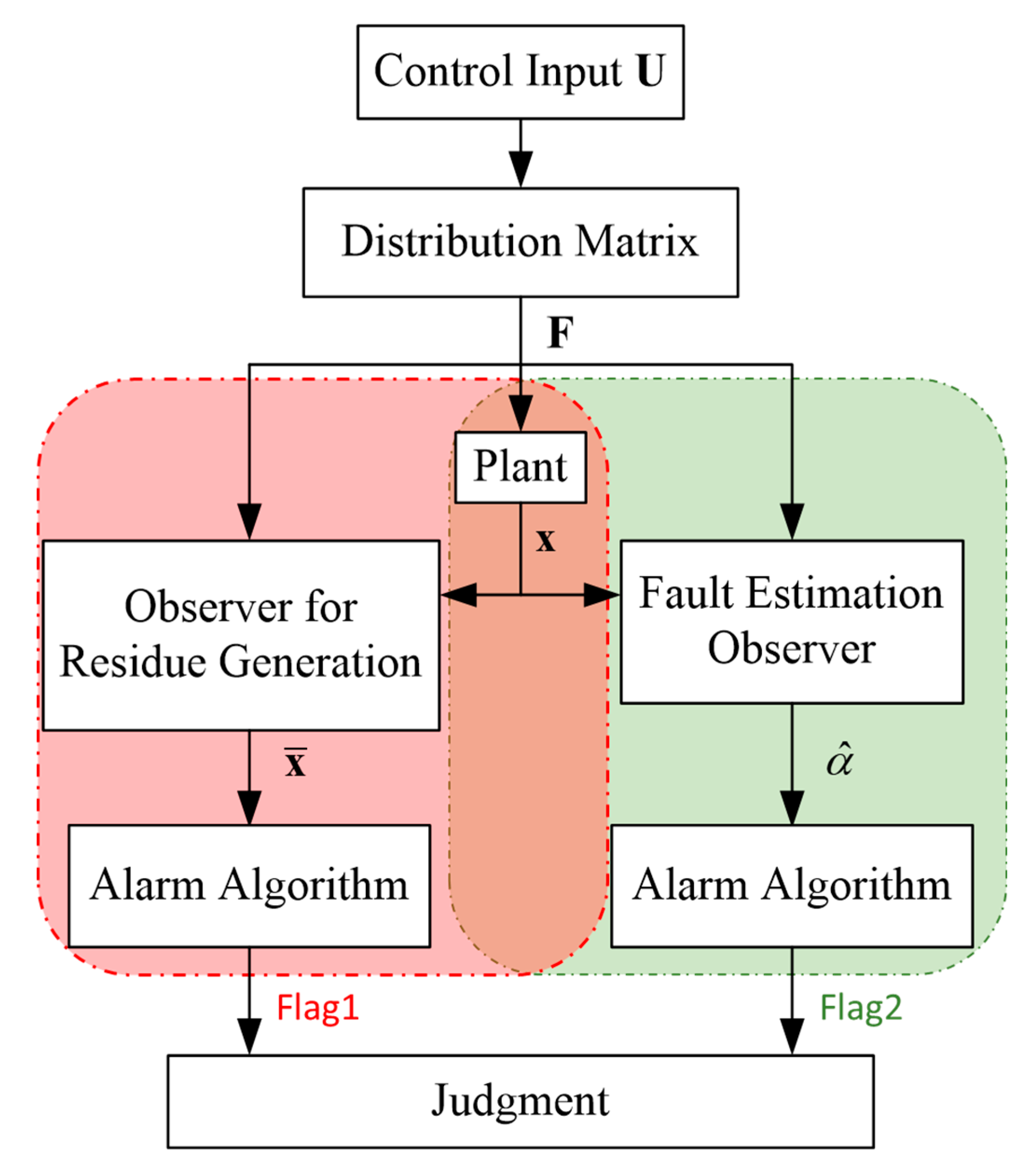
Stability analysis provides a way for the guidance of gain selection of the sliding controller. Define the Lyapunov functions for z-dynamics and Euler angle dynamics respectively as follows:

$$V_z=\frac{1}{2}{s}_z^2$$

(23)

$$V_{\eta }=\frac{1}{2}{\mathbf{s}}_{\eta }^T{\mathbf{s}}_{\eta }$$

(24)

Taking the derivative of Equations (23) and (24) yields:

$$\begin{array}{cc}\hfill {\dot{V}}_z& =-{\rho }_z\frac{{\left|s_z\right|}^2}{\left|s_z\right|+{\epsilon }_z}+\frac{1}{m}\left(f_{wz}-{\delta }_z\dot{z}\right)S_z\le -{\rho }_z\frac{{\left|s_z\right|}^2}{\left|s_z\right|+{\epsilon }_z}+\frac{1}{m}\left(\left|f_{wz}\right|+\left|{\delta }_z\dot{z}\right|\right)\left|s_z\right|\hfill \\ & \le -\frac{\left|s_z\right|}{\left|s_z\right|+{\epsilon }_z}\left({\rho }_z-\frac{1}{m}\left(\left|f_{wz}\right|+\left|{\delta }_z\dot{z}\right|\right)\frac{\left(\left|s_z\right|+{\epsilon }_z\right)}{\left|s_z\right|}\right)\hfill \end{array}$$

(25)

and:

$${\dot{V}}_z=-{\mathsf{\varrho }}_{\eta }\frac{{\Vert {\mathbf{s}}_{\eta }\Vert }^2}{\Vert {\mathbf{s}}_{\eta }\Vert +\Vert {\mathsf{\epsilon }}_{\eta }\Vert }+{\mathbf{s}}_{\eta }^T\mathbf{H}{\mathbf{J}}^{-1}{\mathbf{f}}_{\eta }\le -{\lambda }_{min}\left({\mathsf{\varrho }}_{\eta }\right)\frac{{\Vert {\mathbf{s}}_{\eta }\Vert }^2}{\Vert {\mathbf{s}}_{\eta }\Vert +\Vert {\mathsf{\epsilon }}_{\eta }\Vert }+\Vert {\mathbf{s}}_{\eta }\Vert \Vert \mathbf{H}{\mathbf{J}}^{-1}\Vert \Vert {\mathbf{f}}_{\eta }\Vert$$

(26)

respectively.

Obviously, when the scaling parameter ${\epsilon }_z=0$ and ${\mathsf{\epsilon }}_{\eta }=0$ used in the sigmoid function, Equations (25) and (26) reduce to:

$${\dot{V}}_z=-\left|s_z\right|\left({\rho }_z+\frac{1}{m}\left(\left|f_{wz}\right|+\left|{\delta }_z\dot{z}\right|\right)\right)\le 0$$

(27)

and:

$${\dot{V}}_z\le -\Vert {\mathbf{s}}_{\eta }\Vert \left({\lambda }_{min}\left({\mathsf{\varrho }}_{\eta }\right)-\Vert \mathbf{H}{\mathbf{J}}^{-1}\Vert \Vert {\mathbf{f}}_{\eta }\Vert \right)$$

(28)

It is evident that the finite time approaching is satisfied providing:

$${\rho }_z>\frac{1}{m}\left(\left|f_{wz}\right|+\left|{\delta }_z\dot{z}\right|\right)$$

(29)

$${\lambda }_{\min }\left({\mathsf{\varrho }}_{\eta }\right)>\Vert \mathbf{H}{\mathbf{J}}^{-1}\Vert \Vert {\mathbf{f}}_{\eta }\Vert$$

(30)

The parameters ε_z and ε_η not only eliminate the chattering problem of sliding mode control, but also dominate the convergence capability. Since the traditional discontinuous switching control is replaced by the continuous sigmoid function, the perfect sliding motion may not be attained and the region of the convergence is relative to the size of the scaling parameters used in the sigmoid function. Nevertheless, the high frequency control switching can be avoided.

4. Fault Detection

Model-based fault detection method is discussed in this section. With the implementation of observers, fault alarms could be generated and its residual provides the mechanism for the flight controller switch to the FTC.

4.1. Fault Detection Based on Residue Generation

Define the state variables to be:

$$\mathbf{x}={\left[\begin{array}{cccccccccccc}{x}_1& x_2& x_3& x_4& x_5& x_6& x_7& x_8& x_9& x_{10}& x_{11}& x_{12}\end{array}\right]}^T$$

(31)

where:

$$\begin{gathered} {\left[\begin{array}{cccccc}{x}_1& x_2& x_3& x_4& x_5& x_6\end{array}\right]}^T={\left[\begin{array}{cccccc}\varphi & \theta & \psi & x& y& z\end{array}\right]}^T \\ {\left[\begin{array}{cccccc}{x}_7& x_8& x_9& x_{10}& x_{11}& x_{12}\end{array}\right]}^T={\left[\begin{array}{cccccc}\dot{\varphi }& \dot{\theta }& \dot{\psi }& \dot{x}& \dot{y}& \dot{z}\end{array}\right]}^T \end{gathered}$$

With Equations (2) and (7), the governing equations in state space form could be obtained and written as:

$$\{\begin{array}{l}\dot{\mathbf{x}}=\mathbf{A}\mathbf{x}+\mathbf{h}\left(\mathbf{x}\right)+\mathbf{B}\left(\mathbf{x}\right)\mathsf{\Lambda }\left[\mathbf{I}-\mathsf{\alpha }\right]\mathbf{F}+\mathsf{\gamma }\left(t\right)\\ \mathbf{y}=\mathbf{C}\mathbf{x}\end{array}$$

(32)

where h consists of nonlinear terms, denotes the force distribution matrix, F denotes thrust of each propeller, γ represents disturbance, and α denotes actuator fault residual signal. The rest system matrices are defined as follows:

$$\begin{array}{l}A=\left[\begin{array}{cc}{0}_{6\times 6}& I_{6\times 6}\\ 0_{6\times 6}& 0_{6\times 6}\end{array}\right], h\left(x\right)=\left[\begin{array}{c}{0}_{6\times 1}^{}\\ {\left[\begin{array}{ccc}0& 0& g\end{array}\right]}^T\\ \dot{H}\left(x\right)H^{-1}\left(x\right)\dot{\mathsf{\eta }}-H\left(x\right)J^{-1}P\left(x\right)\end{array}\right], C=I\\ B\left(x\right)=\left[\begin{array}{c}{0}_{6\times 6}\\ \begin{array}{cc}H\left(x\right)J^{-1}& 0_{3\times 3}\end{array}\\ \begin{array}{cc}{0}_{3\times 3}& \frac{1}{m}R\left(x\right)\end{array}\end{array}\right]\left[\begin{array}{cccc}0& 1& 0& 0\\ 0& 0& 1& 0\\ 0& 0& 0& 1\\ 0& 0& 0& 0\\ 0& 0& 0& 0\\ 1& 0& 0& 0\end{array}\right], \mathsf{\alpha }=\left[\begin{array}{cccc}{\alpha }_1& 0& 0& 0\\ 0& {\alpha }_2& 0& 0\\ 0& 0& {\alpha }_3& 0\\ 0& 0& 0& {\alpha }_4\end{array}\right]\\ \mathsf{\Lambda }=\left[\begin{array}{cccc}-1& -1& -1& -1\\ -l_w& l_w& l_w& -l_w\\ -l_l& -l_l& l_l& l_l\\ -\mu & \mu & -\mu & \mu \end{array}\right], h\left(x\right)=\left[\begin{array}{c}{0}_{6\times 1}^{}\\ {\left[\begin{array}{ccc}0& 0& g\end{array}\right]}^T\\ \dot{H}\left(x\right)H^{-1}\left(x\right)\dot{\mathsf{\eta }}-H\left(x\right)J^{-1}P\left(x\right)\end{array}\right], C=I\end{array}$$

Since the system is fully observable, the observer could be designed as follows:

$$\{\begin{array}{l}\dot{\widehat{x}}=A\widehat{x}+h\left(\widehat{x}\right)+B\left(x\right)\mathsf{\Lambda }F+L\left(y-\widehat{y}\right)\\ \widehat{y}=C\widehat{x}\end{array}$$

(33)

where L denotes as the observer gain with proper dimension.

In order to analyze the relationship between the states and the estimated ones, the state estimation error is defined by:

$$\overline{x}=x-\widehat{x}$$

(34)

Taking the derivative of Equation (34), and bringing Equations (32) and (33) into the result gives:

$$\begin{array}{cc}\hfill \dot{\overline{x}}& =\left(A-LC\right)\overline{x}+h\left(x\right)-h\left(\widehat{x}\right)-B\left(x\right)\mathsf{\Lambda }\alpha F+\mathsf{\gamma }\left(x,t\right)\hfill \\ & =A_o\overline{x}+\left[h\left(x\right)-h\left(\widehat{x}\right)\right]-B\left(x\right)\mathsf{\Lambda }\alpha F+\mathsf{\gamma }\left(x,t\right)\hfill \end{array}$$

(35)

where A_o is a negative definite matrix with a proper pole placement via L.

The following assumptions are imposed for the observer stability proof:

Assumption 1.

There exists a positive definite matrix, Q, such that there exists a positive symmetric matrix$\mathsf{\Xi }$, which satisfies$A_o^T\mathsf{\Xi }+\mathsf{\Xi }{A}_o=-Q$.

Assumption 2.

The system satisfies Lipschitz continuity, and there exists a real constant k such that, for all a and b, the property $\Vert f(a)-f(b)\Vert \le \kappa \Vert a-b\Vert$ holds.

Proof. 

Based on Assumptions 1 and 2, define the Lyapunov function as $V={\overline{x}}^T\mathsf{\Xi }\overline{x}$ and take the derivative of it, which gives:

$$\begin{array}{ll}\dot{V}& =-{\overline{x}}^{T}Q\overline{x}+2{\overline{x}}^T\mathsf{\Xi }\left[h\left(x\right)-h\left(\widehat{x}\right)\right]-{\overline{x}}^T\mathsf{\Xi }B\left(x\right)\mathsf{\Lambda }\mathsf{\alpha }F+2{\overline{x}}^T\mathsf{\Xi }\mathsf{\gamma }\left(t\right)\\ & \le -{\lambda }_{\min }\left(Q\right){\Vert \overline{x}\Vert }^2+2{\lambda }_{\max }\left(\mathsf{\Xi }\right)\Vert \overline{x}\Vert \Vert h\left(x\right)-h\left(\widehat{x}\right)\Vert \\ & +2{\lambda }_{\max }\left(\mathsf{\Xi }\right)\Vert \overline{x}\Vert \Vert B\left(x\right)\mathsf{\Lambda }\Vert \Vert F\Vert {\lambda }_{\max }\left(\mathsf{\alpha }\right)+2{\lambda }_{\max }\left(\mathsf{\Xi }\right)\Vert \overline{x}\Vert \Vert \mathsf{\gamma }\left(x,t\right)\Vert \\ & \le -{\lambda }_{\min }\left(Q\right){\Vert \overline{x}\Vert }^2+2{\lambda }_{\max }\left(\mathsf{\Xi }\right){\kappa }_h{\Vert \overline{x}\Vert }^2+2{\lambda }_{\max }\left(\mathsf{\Xi }\right)\Vert \overline{x}\Vert \Vert B\left(x\right)\mathsf{\Lambda }\Vert \Vert F\Vert {\lambda }_{\max }\left(\mathsf{\alpha }\right)\\ & +2{\lambda }_{\max }\left(\mathsf{\Xi }\right)\Vert \overline{x}\Vert \Vert \mathsf{\gamma }\left(x,t\right)\Vert \\ & \le -{\lambda }_{\min }\left(Q\right)\Vert \overline{x}\Vert \left(\Vert \overline{x}\Vert -\frac{2{\lambda }_{\max }\left(\mathsf{\Xi }\right)}{{\lambda }_{\min }\left(Q\right)-2{\lambda }_{\max }\left(\mathsf{\Xi }\right){\kappa }_h}\left(\Vert B\left(x\right)\mathsf{\Lambda }\Vert \Vert F\Vert {\lambda }_{\max }\left(\mathsf{\alpha }\right)+\Vert \mathsf{\gamma }\left(x,t\right)\Vert \right)\right)\end{array}$$

(36)

It can be seen that the estimation error converges as long as $\overline{x}\in \mathsf{\Omega }\left(\overline{x}\right)$:

$$\mathsf{\Omega }\left(\overline{x}\right)=\left\{\begin{array}{rr}\hfill \overline{x}\in {\mathbb{R}}^{12\times 1}& \hfill |\Vert \overline{x}\Vert >\frac{2{\lambda }_{\max }\left(\mathsf{\Xi }\right)}{{\lambda }_{\min }\left(Q\right)-2{\lambda }_{\max }\left(\mathsf{\Xi }\right){\kappa }_h}\left(\Vert B\left(x\right)\mathsf{\Lambda }\Vert \Vert F\Vert {\lambda }_{\max }\left(\mathsf{\alpha }\right)+\Vert \mathsf{\gamma }\left(x,t\right)\Vert \right)\end{array}|\right\}$$

(37)

Equation (37) shows that both the fault signal and external disturbance restrain state estimation error from converging to zero, but to a bound. Hence, the idea of fault detection is to set a boundary of residues. If the residue exceeds the set described by Equation (37), it is regarded as fault happening. To this aim, the work [29] is adopted for boundary generation:

$$r_i^u=\frac{K_{u1i}}{T}{\displaystyle {\int }_{t-T}^t{r}_i\left(\tau \right)d\tau }+\frac{K_{u2i}}{T}{\displaystyle {\int }_{t-T}^t\left(r_i\left(\tau \right)-\frac{1}{T}{\displaystyle {\int }_{\tau -T}^{\tau }{r}_i\left(\beta \right)d\beta }\right)d\tau }+K_{u3i}$$

(38)

$$r_i^{\ell }=\frac{K_{\ell 1i}}{T}{\displaystyle {\int }_{t-T}^t{r}_i\left(\tau \right)d\tau }+\frac{K_{\ell 2i}}{T}{\displaystyle {\int }_{t-T}^t\left(r_i\left(\tau \right)-\frac{1}{T}{\displaystyle {\int }_{\tau -T}^{\tau }{r}_i\left(\beta \right)d\beta }\right)d\tau }-K_{\ell 3i}$$

(39)

Equations (38) and (39) denote the adaptive upper and lower bounds of the residue. r_i denotes the residue along the ith dimension, K_u denotes gains for upper bound, and K_l denotes gains for lower bound. In this study, r_i comes from the state estimation error Equation (34). □

4.2. Fault Detection Based on Fault Estimation

In the previous section, the fault detection method alarms right after the system differs from the model. However, the residue-based fault estimator presented in the previous section is suitable for UAVs with non-static flight orientation. To improve the fault evaluation accuracy for fixed orientation flight situations, another observer for estimating the fault residual is further introduced.

$$\{\begin{array}{l}\dot{\widehat{x}}=A\widehat{x}+h\left(\widehat{x}\right)+B\left(x\right)\mathsf{\Lambda }\left[I-\widehat{\mathsf{\alpha }}\right]F+L\left(y-\widehat{y}\right)\\ \widehat{y}=C\widehat{x}\end{array}$$

(40)

where $\widehat{\mathsf{\alpha }}$ denotes as the estimated fault.

Take the time derivative of Equation (34), consider Equations (32) and (40), one has:

$$\begin{array}{cc}\hfill \dot{\overline{x}}& =\left(A-LC\right)\overline{x}+h\left(x\right)-h\left(\widehat{x}\right)+B\left(x\right)\mathsf{\Lambda }\left[I-\mathsf{\alpha }\right]F-B\left(x\right)\mathsf{\Lambda }\left[I-\widehat{\mathsf{\alpha }}\right]F+\mathsf{\gamma }\left(x,t\right)\hfill \\ & =A_o\overline{x}+\left[h\left(x\right)-h\left(\widehat{x}\right)\right]-B\left(x\right)\mathsf{\Lambda }\tilde{\mathsf{\alpha }}F+\mathsf{\gamma }\left(x,t\right)\hfill \end{array}$$

(41)

To address the stability, the fault is assumed to be slow time varying, and the update rate of estimated fault is designed as:

$${\dot{\widehat{\mathsf{\alpha }}}}_{\Delta }={\rho }_{\alpha }{F}_{\Delta }{\mathsf{\Lambda }}^T{B}^T\left(x\right){\mathsf{\Xi }}^T\overline{x}$$

(42)

where ${\widehat{\mathsf{\alpha }}}_{\Delta }={\left[\begin{array}{cccc}{\widehat{\alpha }}_1& {\widehat{\alpha }}_2& {\widehat{\alpha }}_3& {\widehat{\alpha }}_4\end{array}\right]}^T\in {\mathbb{R}}^{4\times 1}$.

Define a Lyapunov function as $V={\overline{x}}^T\mathsf{\Xi }\overline{x}+{\tilde{\mathsf{\alpha }}}_{\Delta }^T{\tilde{\mathsf{\alpha }}}_{\Delta }/{\rho }_{\alpha }$. Taking the time derivative yields:

$$\begin{array}{ll}\dot{V}& ={\dot{\overline{x}}}^T\mathsf{\Xi }\overline{x}+{\overline{x}}^T\mathsf{\Xi }\dot{\overline{x}}+{\dot{\tilde{\mathsf{\alpha }}}}_{\Delta }^T{\tilde{\mathsf{\alpha }}}_{\Delta }/{\rho }_{\alpha }+{\tilde{\mathsf{\alpha }}}_{\Delta }^T{\dot{\tilde{\mathsf{\alpha }}}}_{\Delta }/{\rho }_{\alpha }\\ & =-{\overline{x}}^{T}Q\overline{x}+2{\overline{x}}^T\mathsf{\Xi }\left(h\left(x\right)-h\left(\widehat{x}\right)\right)+2{\overline{x}}^T\mathsf{\Xi }\mathsf{\gamma }\left(x,t\right)-2\left({\overline{x}}^T\mathsf{\Xi }B\left(x\right)\mathsf{\Lambda }{F}_{\Delta }+{\dot{\widehat{\mathsf{\alpha }}}}_{\Delta }^T/{\rho }_{\alpha }\right){\tilde{\mathsf{\alpha }}}_{\Delta }\\ & =-{\overline{x}}^{T}Q\overline{x}+2{\overline{x}}^T\mathsf{\Xi }\left(h\left(x\right)-h\left(\widehat{x}\right)\right)+2{\overline{x}}^T\mathsf{\Xi }\mathsf{\gamma }\left(x,t\right)\\ & \le -{\lambda }_{\min }\left(Q\right){\Vert \overline{x}\Vert }^2+2{\lambda }_{\max }\left(\mathsf{\Xi }\right)\kappa {\Vert \overline{x}\Vert }^2+2{\lambda }_{\max }\left(\mathsf{\Xi }\right)\Vert \overline{x}\Vert \Vert \mathsf{\gamma }\left(x,t\right)\Vert \end{array}$$

(43)

The inequality implies that the convergence of state estimation error is affected by the external disturbance:

$$\Vert \overline{x}\Vert \ge \frac{2{\lambda }_{\max }\left(\mathsf{\Xi }\right)}{{\lambda }_{\min }\left(Q\right)-2{\lambda }_{\max }\left(\mathsf{\Xi }\right)\kappa }\Vert \mathsf{\gamma }\left(x,t\right)\Vert$$

(44)

The result of fault estimation is affected by the state estimation error. Thus, the observer gain should be selected carefully in case of making a fault estimation stop updating. On the other hand, the convergence of state estimation error is affected by the magnitude of the disturbance, which also has an impact on the fault estimation precision. The next step is to address the mechanism for the determination of the rotor fault.

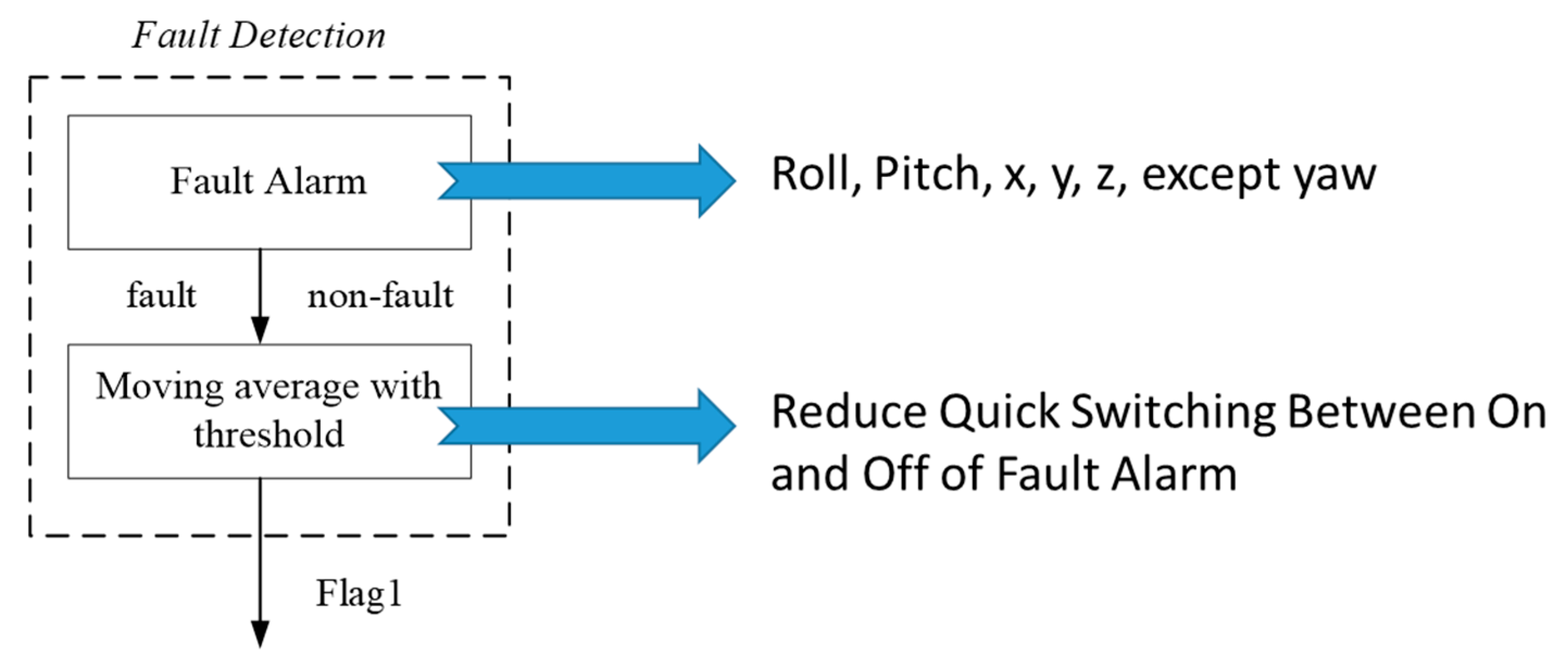
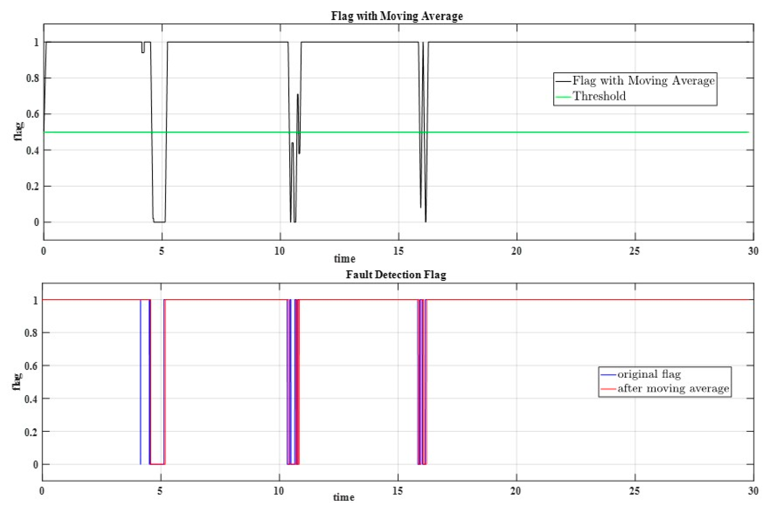
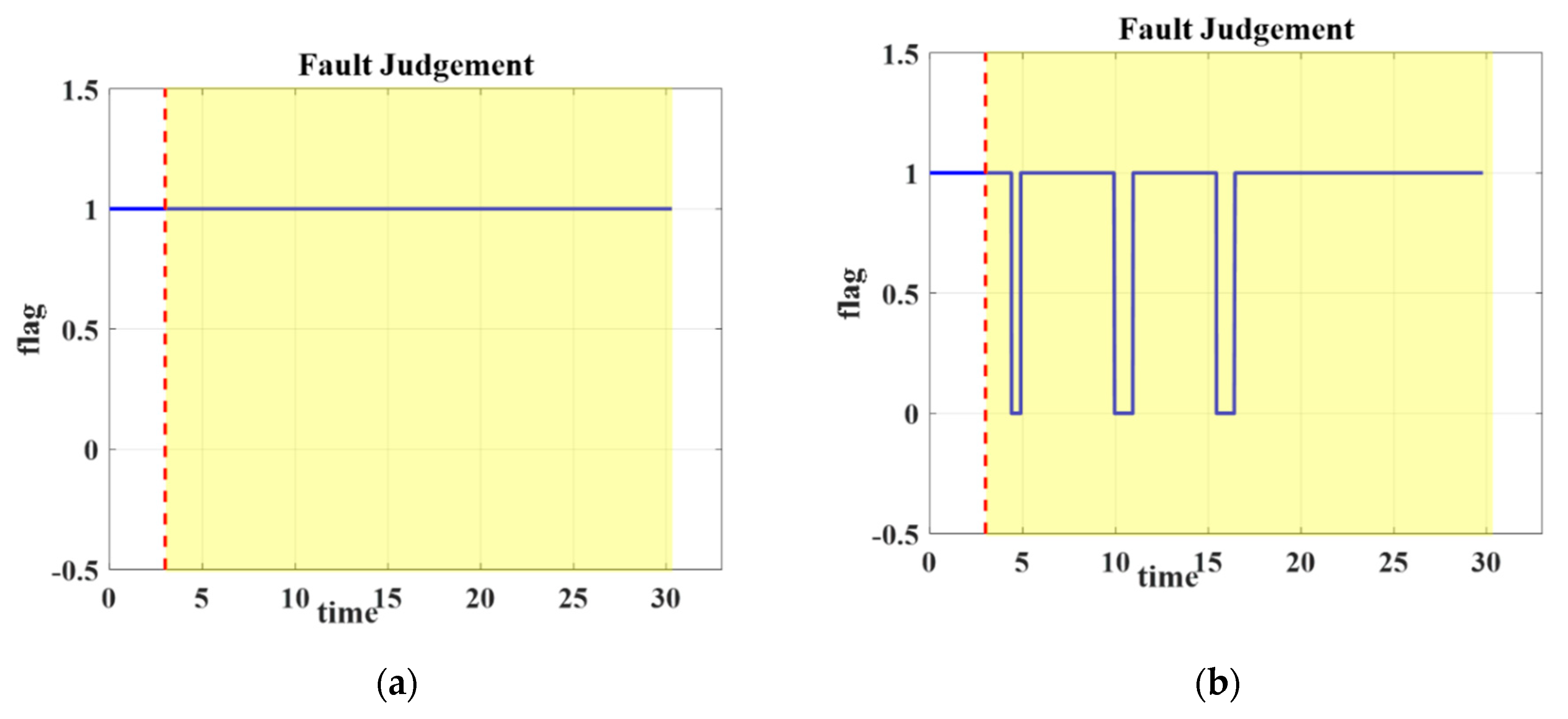
4.3. Fault Detection Making Algorithm

Based on the dual observers as shown in Figure 4, they return two flags. Flag1 and Flag2 represent the judgement results from the methods presented in the Section 4.1 and Section 4.2, respectively. As for Flag1, the residues of roll, pitch, x, y, and z are taken into consideration. When any of the residues mentioned exceeds the upper bound or lower bound as presented in Equations (38) and (39), the fault alarm Flag1 would be triggered. However, using only Flag1 would lead to an incorrect fault alarm. As for Flag2, the estimated fault would be filtered by moving average. If any of the results exceed the threshold, it is treated as fault happening. The fault signal of from the 1st observer reacts quickly when fault happens, but residues may still converge due to the property of observer. The fault signal of the 2nd observer requires time to converge while it would eventually close to the fault happening. With the combination of Flag1 and Flag2, the decision making regarding whether the true fault happens or not would be made in the judgment block as shown in Figure 4. By default, Flag1 = Flag2 = 1, which represents the normal status. Therefore, the real-time fault double confirmation procedure, as shown in

Table 1. Rotor fault judgement procedure.

if   Flag1 || Flag2 == 0 => Fault_True = 1

if   Fault_True == 1

if   Flag1 && Flag2 == 1 holds for 0.5 sec

→Fault_True = 0 and reset Flag1=Flag2=1;

→return status is considered as normal

else

→return status is considered as a rotor fault

, is applied:

Based on the judgement procedure, if any of the flags denotes a fault is happening, the fault detection result would be considered as a fault happening first. In order to prevent wrong judgments, a mechanism is further imposed to pull back a faulty alarm. That is, if both of the flags denote normal flight for a time period, the fault detection would return to “normal”.

5. Simulation Results

To verify the proposed fault detection and fault control strategies, in the following sections we consider a couple of simulations.

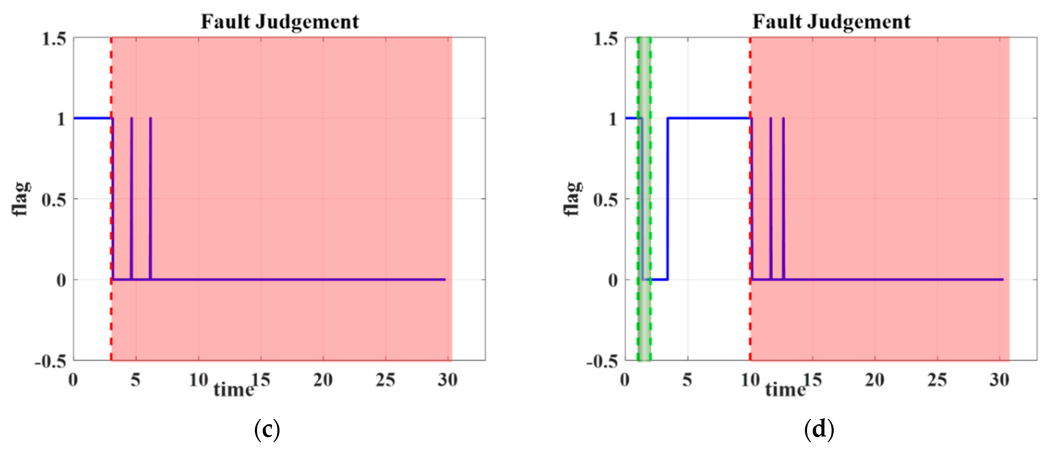
5.1. Fault Detection Results

Figure 5 shows the detailed signal processing of residual-based fault detection. The yaw residue result is not considered, since it is sensitive to the unexpected yaw motion induced by loss of efficiency (LOE) or rotor failure. In our case, slight LOE is not classified to an actuator fault since the quadrotor at this situation still has the ability to complete the flight mission. Parameters for the upper and lower boundary discussed in Section 4.1 are set to be

Table 2. Gain selections for the adaptive residue boundary.

		Lower Bound			Upper Bound			T(s)
State		${\mathit{K}}_{\ell 1\mathit{i}}$	${\mathit{K}}_{\ell 2\mathit{i}}$	${\mathit{K}}_{\ell 3\mathit{i}}$	${\mathit{K}}_{\mathit{u}1\mathit{i}}$	${\mathit{K}}_{\mathit{u}2\mathit{i}}$	${\mathit{K}}_{\mathit{u}3\mathit{i}}$
$\varphi$, $\theta$		1	0.05	0.0004	1	0.05	0.0004	0.015
$x$, $y$, $z$		1	0.05	0.002	1	0.05	0.002	0.015

.

In Figure 6, the fault is detected at 4.12 s when it is set to happen at 3.9 s, where the blue and black lines represent $r_i^u$ and $r_i^{\ell }$, respectively. The reaction time is about 0.22 s with the parameter set in Table 2. After getting result, the fault signal would be filtered by a moving average.

In order to prevent outliers during the fault estimation process, the moving average method is also applied, where the parameters are shown in

Table 3. Parameters of the moving average.

Method	Moving Window	Threshold
residue estimation from the 1st observer	0.01 (s)	0.5
fault estimation from the 2nd observer	0.1 (s)	0.7

. The fault estimation method performs well under slow time varying fault. Meanwhile, with the implement of moving average, the chance of accidental triggering of fault alarm could be reduced.

As the fault signal is being processed by moving average, the threshold illustrated in Table 3 would separate the result into Boolean logic answers that represent whether a fault happened or not. In Figure 7, it is regarded as normal flight when the Flag is 1. Due to the convergent property of the observer, a fault detection result based on residue generation is accurate only around the time that the fault happens. As one can see, some switching between normal and abnormal judgment appears around the fault occurrence time. After taking a moving average, the fault detection results act much better.

As one could see in Figure 8, the estimated fault becomes smoother, which reduces the chance of accidental triggering.

On the other hand, the control law of the quadrotor would be modified, which releases yaw control, right after a fault happens. The unexpected yaw motion would affect the fault estimation result. Thus, the strategy is to take the biggest component of the estimated fault and examine it by using a threshold. In Figure 9, it is regarded as a fault happening when the estimated fault exceeds the threshold.

Figure 10 shows fault judgement results of different cases. The solid line denotes the flag representing the result of the fault judgement, where the Boolean ‘1’ represents normal flight, and ‘0’ represents a detected fault. The transparent blocks are the time when the fault condition is acting on the rotor, where the yellow one denotes the LOE case, and the red one denotes the rotor broken case. The transparent green region denotes the time when a gust disturbance is acting as a perturbation on the quad-rotor.

In Figure 10a, the fault happens at 3 s. It can be seen that the 20% LOE doesn’t trigger the fault alarm since its effect to the motion of the quad-rotor is not serious. Hence, it is treated as a case of uncertainty. In Figure 10b, the fault happens at 3 s, which is highlighted by the transparent yellow block. During the 60% LOE of one rotor, the fault alarm is triggered at approximately the 5, 10, and 15 s, which are the time when quad-rotor is flying passing through the wait points and changing the attitude for the next tracking target.

Due to the medium fault level of rotor, some motion with large attitude change of the quad-rotor would trigger the fault alarm. Nonetheless, the judgement of FDI returns to the normal flight successfully within the smooth flight periods. In Figure 10c, the fault happens at 3 s, which has been highlighted by the transparent red block. As one could see, the fault has been detected immediately after the rotor failure, which guarantees the safety flight of the quad-rotor. The result is acceptable, though there are some switching periods during the time the fault is happening. These are the result of a tradeoff between the correction for misjudgment of the FDI, which returns the fault control to the normal one, and the safety concern, which maintains the fault tolerant control. Nonetheless, the switching times are actually quite few that would not affect the safe flight of the quad-rotor. In Figure 10d, the perturbation caused by disturbance is shown within the 1 to 2 s, which is covered by the green block, and the fault happens at 10 s that last until the end of simulation.

As discussed before, the fault detection result would be affected by disturbances, which means misjudgment is inevitable. Nevertheless, with the proposed algorithm, the control law would be switched back to the normal one in a short period after the perturbation. Meanwhile, the short period that treated as fault happening would not be regarded as rotor fault, but rather as an external disturbance.

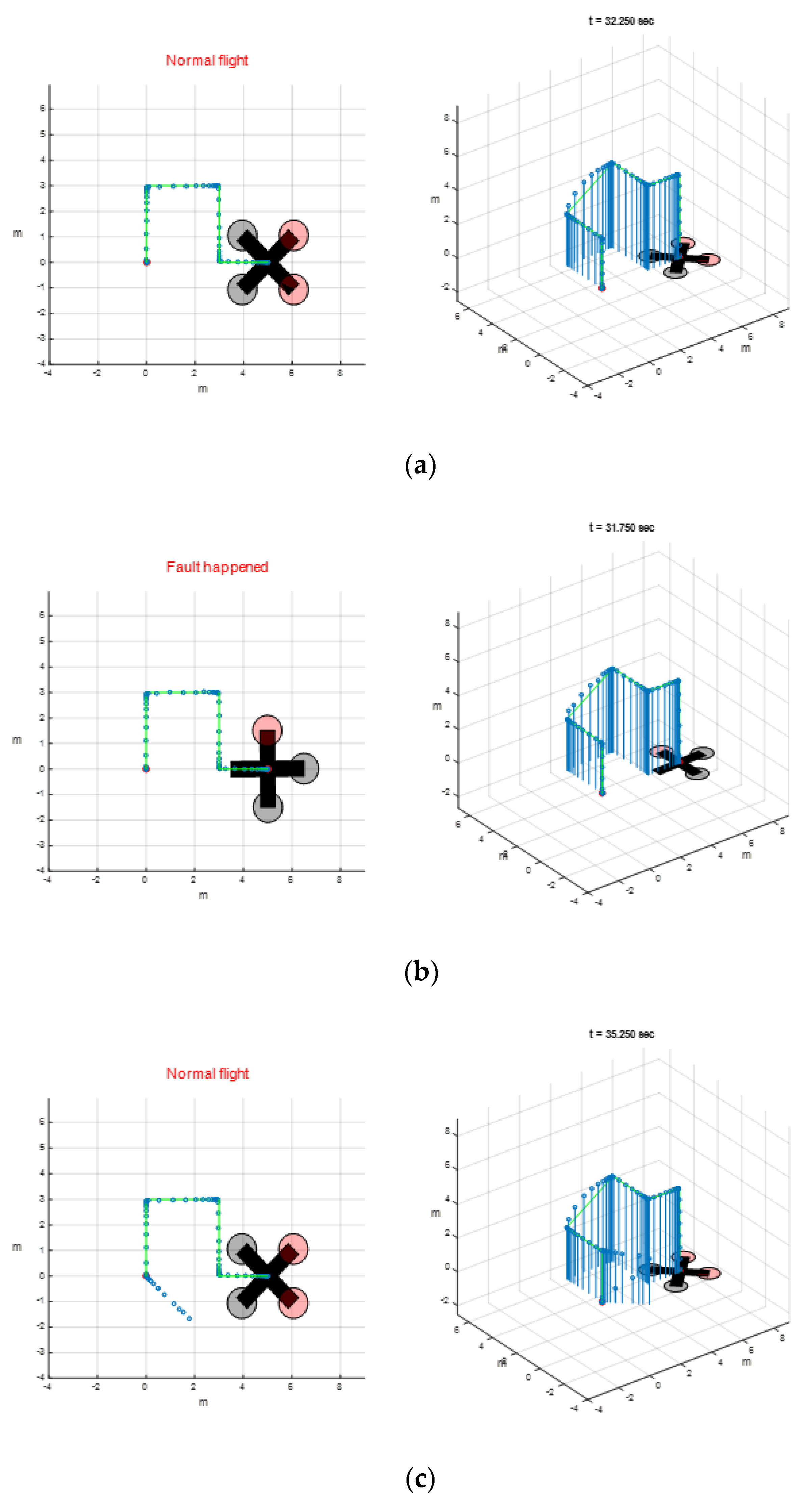
5.2. Quadcotor Flight Simulation with Rotor Fault

In the following, the flight behavior by using the proposed fault tolerance control strategies is visualized. Figure 11 shows the demonstration of flying path of the quad-rotor for simulation. Each corner between green lines represents the way point. To provide a smooth flight path, velocity as well as acceleration, the flight trajectories between each way point are generated by applying a second order low pass filter.

Figure 12a shows the normal flight. Figure 12b shows that the quadrotor performs well even when a fault happens. Figure 12c represents a robust flight for the quadrotor in the face of an external wind disturbance. As one could see, the final state of fault judgment is normal flight, which means the control law is switched back to the normal one even when the disturbance has been treated as a fault. Finally, in Figure 12d, the quadrotor successfully completes the flight mission even in the presence of a rotor fault as well as an external wind disturbance. The associated flight dynamic simulation can refer to the Supplementary Material.

6. Conclusions

This paper proposed a strategy for quadrotor flight control for a single rotor failure. Under this circumstance, the developed flight strategy consists of normal and abnormal control modes. Therefore, the fault detection scheme, including fault detection and estimation used to determine current flight condition, plays an important role in our FTC strategy. To prevent an incorrect alarm from misjudgment of an actuator fault, the algorithm not only determines the fault alarm, but also provides a fault confirmation mechanism to rise the confidence of the fault decision making process. On the other hand, to provide robust flight control under external wind perturbation conditions, sliding mode control theory is considered. Most importantly, to deal with a drone flight subject to rotor failure, a real-time coordinate transformation-based control scheme is developed. This method is able to guarantee not only the stable flight under spinning motion, but completion of the prescribed flight task as well.

References

1. Yungaicela-Naula, N.; Garza-Castañon, E.L.; Zhang, Y.; Minchala-Avila, I.L. Uav-based air pollutant source localization using combined metaheuristic and probabilistic methods. Appl. Sci. 2019, 9, 3712. [Google Scholar] [CrossRef] [Green Version]
2. Tabbache, B.; Benbouzid, M.E.H.; Kheloui, A.; Bourgeot, J. Virtual-sensor-based maximum-likelihood voting approach for fault-tolerant control of electric vehicle powertrains. IEEE Trans. Veh. Technol. 2013, 62, 1075–1083. [Google Scholar] [CrossRef] [Green Version]
3. Kommuri, S.K.; Defoort, M.; Karimi, H.R.; Veluvolu, K.C. A robust observer-based sensor fault-tolerant control for pmsm in electric vehicles. IEEE Trans. Ind. Electron. 2016, 63, 7671–7681. [Google Scholar] [CrossRef]
4. Marino, R.; Scalzi, S.; Tomei, P.; Verrelli, C.M. Fault-tolerant cruise control of electric vehicles with induction motors. Control Eng. Pract. 2013, 21, 860–869. [Google Scholar] [CrossRef]
5. Jin, J.; Youmin, Z. Accepting performance degradation in fault-tolerant control system design. IEEE Trans. Control Syst. Technol. 2006, 14, 284–292. [Google Scholar]
6. Slotine, J.-J.E.; Li, W. Applied Nonlinear Control; Prentice Hall Englewood Cliffs: Bergen County, NJ, USA, 1991; Volume 199. [Google Scholar]
7. Youmin, Z.; Jin, J. Fault tolerant control system design with explicit consideration of performance degradation. IEEE Trans. Aerosp. Electron. Syst. 2003, 39, 838–848. [Google Scholar] [CrossRef] [Green Version]
8. Aravena, J.; Zhou, K.; Li, X.R.; Chowdhury, F. Fault tolerant safe flight controller bank 1. IFAC Proc. Vol. 2006, 39, 807–812. [Google Scholar] [CrossRef]
9. Boskovic, J.D.; Mehra, R.K. A Multiple Model-Based Reconfigurable Flight Control System Design. In Proceedings of the 37th IEEE Conference on Decision and Control (Cat. No.98CH36171), Tampa, FL, USA, 16–18 December 1998; Volume 4504, pp. 4503–4508. [Google Scholar]
10. Gopinathan, M.; Boskovic, J.D.; Mehra, R.K.; Rago, C. A Multiple Model Predictive Scheme for Fault-Tolerant Flight Control Design. In Proceedings of the 37th IEEE Conference on Decision and Control (Cat. No.98CH36171), Tampa, FL, USA, 16–18 December 1998; Volume 1372, pp. 1376–1381. [Google Scholar]
11. Kanev, S.; Verhaegen, M. A bank of reconfigurable lqg controllers for linear systems subjected to failures. In Proceedings of the 39th IEEE Conference on Decision and Control (Cat. No.00CH37187), Sydney, NSW, Australia, 12–15 December 2000; Volume 3684, pp. 3684–3689. [Google Scholar]
12. Narendra, K.S.; Balakrishnan, J. Adaptive control using multiple models. IEEE Trans. Autom. Control 1997, 42, 171–187. [Google Scholar] [CrossRef]
13. Narendra, K.S.; Driollet, O.A. Adaptive control using multiple models, switching, and tuning. In Proceedings of the IEEE 2000 Adaptive Systems for Signal Processing, Communications, and Control Symposium (Cat. No.00EX373), Lake Louise, AB, Canada, 4 October 2000; pp. 159–164. [Google Scholar]
14. Freddi, A.; Lanzon, A.; Longhi, S. A feedback linearization approach to fault tolerance in quadrotor vehicles. IFAC Proc. Vol. 2011, 44, 5413–5418. [Google Scholar] [CrossRef] [Green Version]
15. Hess, R.A.; Wells, S.R. Sliding mode control applied to reconfigurable flight control design. J. Guid. Control Dyn. 2003, 26, 452–462. [Google Scholar] [CrossRef]
16. Alwi, H.; Edwards, C. Lpv sliding mode fault tolerant control of an octorotor using fixed control allocation. In Proceedings of the 2013 Conference on Control and Fault-Tolerant Systems (SysTol), Nice, France, 9–11 October 2013; pp. 772–777. [Google Scholar]
17. Edwards, C.; Chen, L.; Khattab, A.; Alwi, H.; Sato, M. Flight Evaluations of Sliding Mode Fault Tolerant Controllers. In Proceedings of the 15th International Workshop on Variable Structure Systems (VSS) Graz University of Technology, Graz, Austria, 9–11 July 2018; pp. 180–185. [Google Scholar]
18. Hamayun, M.T.; Edwards, C.; Alwi, H. Fault Tolerant Control Schemes Using Integral Sliding Modes; Springer AG: Basel, Switzerland, 2016. [Google Scholar]
19. Zou, Y.; Zhu, B. Adaptive trajectory tracking controller for quadrotor systems subject to parametric uncertainties. J. Frankl. Inst. 2017, 354, 6724–6746. [Google Scholar] [CrossRef]
20. Thirumarimurugan, M.; Bagyalakshmi, N.; Paarkavi, P. Comparison of fault detection and isolation methods: A review. In Proceedings of the 2016 10th International Conference on Intelligent Systems and Control (ISCO), Coimbatore, India, 7–8 January 2016; pp. 1–6. [Google Scholar]
21. Guo, D.; Wang, Y.; Zhong, M.; Zhao, Y. Fault detection and isolation for unmanned aerial vehicle sensors by using extended pmi filter. IFAC-PapersOnLine 2018, 51, 818–823. [Google Scholar] [CrossRef]
22. Freddi, A.; Longhi, S.; Monteriù, A. A Model-Based Fault Diagnosis System for a Mini-Quadrotor. In Proceedings of the 7th Workshop on Advanced Control and Diagnosis (ACD), Zielona Gora, Poland, 19–20 November 2009; pp. 1–6. Available online: http://www.issi.uz.zgora.pl/ACD_2009/program/Papers/58_ACD_2009.pdf (accessed on 16 October 2009).
23. Ghalamchi, B.; Mueller, M. Vibration-based propeller fault diagnosis for multicopters. In Proceedings of the 2018 International Conference on Unmanned Aircraft Systems (ICUAS), Dallas, TX, USA, 12–15 June 2018; pp. 1041–1047. [Google Scholar]
24. Boudjedir, H.; Bouhali, O.; Rizoug, N. Adaptive neural network control based on neural observer for quadrotor unmanned aerial vehicle. Adv. Robot. 2014, 28, 1151–1164. [Google Scholar] [CrossRef]
25. Li, C.; Zhang, Y.; Li, P. Extreme learning machine based actuator fault detection of a quadrotor helicopter. Adv. Mech. Eng. 2017, 9, 1687814017705068. [Google Scholar] [CrossRef]
26. Monteriù, A.; Asthana, P.; Valavanis, K.; Longhi, S. Real-time model-based fault detection and isolation for ugvs. J. Intell. Robot. Syst. 2009, 56, 425–439. [Google Scholar] [CrossRef]
27. Avram, R.C.; Zhang, X.; Muse, J. Quadrotor actuator fault diagnosis and accommodation using nonlinear adaptive estimators. IEEE Trans. Control Syst. Technol. 2017, 25, 2219–2226. [Google Scholar] [CrossRef]
28. Avram, R.C. Fault Diagnosis and Fault-Tolerant Control of Quadrotor Uavs. Ph.D. Thesis, Wright State University, Dayton, OH, USA, 2016. [Google Scholar]
29. Longhi, S. A diagnostic thau observer for a class of unmanned vehicles. J. Intell. Robot. Syst. 2012, 67, 61–73. [Google Scholar]
30. Cen, Z.; Noura, H.; Susilo, T.B.; Younes, Y.A. Robust fault diagnosis for quadrotor uavs using adaptive thau observer. J. Intell. Robot. Syst. 2014, 73, 573–588. [Google Scholar] [CrossRef]
31. Ganguli, S.; Marcos, A.; Balas, G. Reconfigurable lpv control design for boeing 747-100/200 longitudinal axis. In Proceedings of the 2002 American Control Conference (IEEE Cat. No.CH37301), Anchorage, AK, USA, 8–10 May 2002; Volume 3615, pp. 3612–3617. [Google Scholar]
32. López-Estrada, F.R.; Ponsart, J.-C.; Theilliol, D.; Zhang, Y.; Astorga-Zaragoza, C.-M. Lpv model-based tracking control and robust sensor fault diagnosis for a quadrotor uav. J. Intell. Robot. Syst. 2016, 84, 163–177. [Google Scholar] [CrossRef]
33. Nguyen, N.P.; Hong, S.K. Sliding mode thau observer for actuator fault diagnosis of quadcopter uavs. Appl. Sci. 2018, 8, 1893. [Google Scholar] [CrossRef] [Green Version]
34. Ortiz-Torres, G.; Castillo, P.; Sorcia-Vázquez, F.D.J.; Rumbo-Morales, J.Y.; Brizuela-Mendoza, J.A.; Cruz-Soto, J.D.L.; Martínez-García, M. Fault estimation and fault tolerant control strategies applied to vtol aerial vehicles with soft and aggressive actuator faults. IEEE Access 2020, 8, 10649–10661. [Google Scholar] [CrossRef]
35. Lei, Y.; Wang, H. Aerodynamic optimization of a micro quadrotor aircraft with different rotor spacings in hover. Appl. Sci. 2020, 10, 1272. [Google Scholar] [CrossRef] [Green Version]
36. Lee, U.K.; Choi, H.Y.; Park, B.J. Inverse optimal design for position control of a quadrotor. Appl. Sci. 2017, 7, 907. [Google Scholar] [CrossRef] [Green Version]
37. Chaturvedi, N.A.; Sanyal, A.K.; McClamroch, N.H. Rigid-body attitude control. IEEE Control Syst. Mag. 2011, 31, 30–51. [Google Scholar]
38. Mueller, M.W.; Andrea, R.D. Stability and control of a quadrocopter despite the complete loss of one, two, or three propellers. In Proceedings of the 2014 IEEE International Conference on Robotics and Automation (ICRA), Hong Kong, China, 31 May–7 June 2014; pp. 45–52. [Google Scholar]
Figure 1. Quad-rotor dimension assumption.
Applsci 10 03503 g001
Figure 2. Definitions of the Quadrotor: (a) thrust directions; (b) spin direction of the propellers.
Applsci 10 03503 g002
Figure 3. Fault-tolerant control strategy.
Applsci 10 03503 g003
Figure 4. Fault detection scheme.
Applsci 10 03503 g004
Figure 5. Flow chart of residue based fault detection process.
Applsci 10 03503 g005
Figure 6. Residual responses for fault detection.
Applsci 10 03503 g006
Figure 7. Fault signal filtered by moving average.
Applsci 10 03503 g007
Figure 8. Comparison of fault estimation with estimated fault processed by a moving average.
Applsci 10 03503 g008
Figure 9. Judgement of fault estimation result.
Applsci 10 03503 g009
Figure 10. Fault judgement results: (a) 20% fault in the second rotor; (b) 60% fault in the second rotor; (c) 100% fault in the second rotor; (d) 100% fault in the second rotor with short period gust disturbance.
Applsci 10 03503 g010aApplsci 10 03503 g010b
Figure 11. Demonstration of flying path with connected wait points.
Applsci 10 03503 g011
Figure 12. Simulation results: (a) normal flight; (b) fault happens at 11 s; (c) disturbance happens at 1–3 s; (d) combination of (b,c).
Applsci 10 03503 g012aApplsci 10 03503 g012b